and Gershwin (1978) proposed a new Markov state model more accurate than .... standard operation partition to the buffer drainage one, and T drainâstd to the ...
Noname manuscript No. (will be inserted by the editor)
Discrete time model for two-machine one-buffer transfer lines with restart policy Elisa Gebennini · Andrea Grassi · Cesare Fantuzzi · Stanley B. Gershwin · Irvin C. Schick
Received: date / Accepted: date
Abstract The paper deals with analytical modeling of transfer lines consisting of two machines decoupled by one finite buffer. In particular, the case in which a control policy (referred as “restart policy”) aiming to reduce the blocking frequency of the first machine is addressed. Such a policy consists of forcing the first machine to remain idle (it cannot process parts) each time the buffer gets full until it empties again. This specific behavior can be found in a number of industrial production systems, especially when some machines are affected by outage costs when stops occur. The two-machine one-buffer line is here modeled as a discrete time markov process and the two machines are characterized by the same production rate. The analytical solution of the model is obtained and mathematical expressions of the most important performance measures are provided. Some significant remarks about the effect of the proposed restart policy on the behavior of the system are also pointed out. Keywords Transfer line · Restart policy · Stochastic model · Performance estimation
1 Introduction Production and transfer lines basically consist of series of machines able to perform specific operations on raw material at a predefined processing rate. Such a configuration is widely adopted in the industrial field, especially when high demand volumes and process repetitiveness have to be assured. Elisa Gebennini, Andrea Grassi, Cesare Fantuzzi Dipartimento di Scienze e Metodi dell’Ingegneria, Universit`a degli Studi di Modena e Reggio Emilia Via Amendola 2 – Pad. Morselli, 42122 Reggio Emilia, Italy Stanley B. Gershwin Laboratory for Manufacturing and Productivity – MIT Department of Mechanical Engineering Massachusetts Institute of Technology 77 Massachusetts Avenue, Cambridge, Massachusetts 02139, USA Irvin C. Schick Faculty of Engineering and Natural Sciences Sabanci University Tuzla Istanbul 34956, Turkey
2
The performance of such a structured manufacturing system is hugely related to the reliability of the process executed by the machines. Actually, unpredictable jamming events (referred as “failures” in the sequel) can occur on machines, producing unwanted stops and causing the need for manual interventions to restore the operational state. In addition, since the system is configured as a line, a failure occurring on a specific machine can propagate its effects also to the other machines located both in the upstream and in the downstream. We refer to a “starvation” when an operational machine is found in idle state as a consequence of an interruption of its incoming flow, and to a “block” when its outgoing flow is prevented. Hence, the efficiency of the whole system is not only related to the reliability of the very machines, but also to the harmful interactions among them. Buffers can be positioned along the line in such a way as to reduce efficiency losses due to machine interactions. Buffers can avoid starvation and blocking of machines by accumulating and releasing material. The most important aspect in the design of a production/transfer line is to be able to relate machine reliability targets and buffer allocation to the performance of the line. Given the random nature of the phenomena involved in the behavior of such manufacturing systems, a stochastic approach is needed to obtain suitable mathematical models. For several decades scientists have produced a lot of work concerning stochastic modeling of production/transfer lines, and a wide survey is reported in Section 2. In all of these works, buffers are considered to run without any kind of control, that is, they can accept material if they are not full and they can release material if they are not empty. Hence, the machine in the immediate upstream of the buffer is allowed to discharge material each time the buffer is not full, while the machine in the immediate downstream is allowed to withdraw material each time the buffer is not empty. On the contrary, in this paper we introduce a restart policy on the first machine in order to reduce its blocking frequency. In fact, in some kind of industrial manufacturing systems, it can happen that some machines undergo an outage cost each time they stop, as a consequence of either internal failures or blocking events in the downstream flow. The outage cost is due to the particular technological process machines execute. In general, machines performing a continuous process are hugely affected by outage costs as a consequence of waste production at each restart. It is of evidence that stops on such machines must be kept to a bare minimum. While the reduction of jamming stops can be obtained only directly acting on the failure rate of the machine itself, a reduction in those stops due to the blocking of the outgoing flow can be obtained by adding a buffer in the immediate downstream and by introducing a proper control policy. Hence, in the present work, we assume that the machine affected by outage costs is the first one in the two-machine one-buffer sub-system. A control policy, referred as restart policy in the sequel, is applied. The restart policy presented in this paper acts each time the buffer gets full and, consequently, the first machine gets blocked because its outgoing flow is interrupted. Specifically, the first machine is put into the so-called “controlled idle state”, i.e. it is forced to remain idle even when the buffer level starts to decrease. The “controlled idle state” on the first machine persists until the buffer empties again. The aim of such a restart policy is to reduce the probability of a further block on the first machine (and, consequently, of a further outage cost) if the downstream machine fails again when the buffer level is still high, i.e. the actual accumulation capacity is still low. Thus, the main contribution of the present work involves the development of a discrete time Markov model for the two-machine one-buffer transfer line with a restart policy. Such an innovative model allows to reproduce the real behavior of many manufacturing systems. It can provide estimations of the line throughput and efficiency, and also a measure of the
3
blocking frequency of the first machine. This latter measure is very important since it directly affects outage costs. The remaider of the paper is organized as follows. Section 2 widely analyzes the scientific literature about the subject. Section 3 clarifies the notation adopted throughout the paper. Section 4 formalizes the proposed model. In Sections 5 and 6 model equations and performance measures are developed, while in Section 7 the analytical solution is obtained. Finally, Section 8 provides some numerical results and discussions, and Section 9 points out some concluding remarks.
2 Literature Review We refer to a manufacturing system as a transfer line if parts are transported between work stations simultaneously, as a production line if each part moves independently of other parts among the work stations. Papadopoulos and Heavey (1996) provide a useful classification of analytical approaches for production and transfer lines modeling. For extensive reviews, the reader can also refer to Dallery and Gershwin (1992) and textbooks as Papadapoulos et al (1993) and Gershwin (2002). The model presented in this paper deals with transfer lines. In Papadopoulos and Heavey (1996) the authors distinguish between generative models and evaluative models. Generative models provide the user with an optimal (or near-optimal) solution which correspond to the maximization/minimization of a predefined objective function. Frequently the problem is to allocate buffer space along the line in order to minimize the work-inprocess or maximize the throughput: we refer to this situation as the buffer allocation problem. Examples of generative methods are the traditional segmentation methods (such as the Hooke-Jeeves method), various heuristics (Papadopoulos and Vidalis, 1998, 1999, 2001a,b), genetic algorithms (Bulgak et al, 1995) and approaches using gradient method (Gershwin and Schor, 2000), simulated annealing (Spinellis and Papadopoulos, 2000), and tabu search (Lutz et al, 1998). Evaluative models consider a given set of input data to provide the user with performance measures rather than with an optimal solution. This paper falls into this second category. Note that, generally, generative models use evaluative models in order to compute the value of the objective function for a given system configuration and then search for an optimal solution. Thus, appropriately formulated evaluative models allow to develop generative models in a combined “closed loop” configuration (Papadopoulos and Heavey, 1996; Spinellis and Papadopoulos, 2000). According to the classification proposed by Papadopoulos and Heavey (1996), models regarding transfer and production lines have to be classified on the basis of failure types. In particular, two types of failures can be considered: operation-dependent failures (i.e. a machine can fail only if it is operational) or time-dependent failures. The proposed model assumes operation-dependent failures. Exact models dealing with transfer lines are available only for small lines. Buzacott (1967) modeled a system characterized by two machines separated by a single finite buffer as a Markov process. Buzacott and Hanifin (1978) justified the assumption of operationdependent failures and derived the expression of the efficiency of such a transfer line. Schick and Gershwin (1978) proposed a new Markov state model more accurate than Buzacott (1967). The same authors provided also a model for three-machine and two-buffer transfer lines (Gershwin and Schick, 1983).
4
Since then, much of the literature has been devoted to two main objectives. The first objective is to extend exact models in order to consider more general distributions (e.g. exponential and phase-type distributions) for both the reliability parameters and the service times allowing to treat also asynchronous and non-homogeneous lines (i.e. production lines, as named in this paper). For example Buzacott (1972), Altiok and Stidham (1983), and Gershwin and Berman (1981) obtained models for the two-machine one-buffer system in which service times are exponentially distributed. In Berman (1982) the service time for the two machines is assumed to be Erlang with K (K ≥ 1) phases. Nevertheless, a better approximation of asynchronous non-homogeneous lines can be achieved by continuous models, originally proposed by Zimmern (1956). Gershwin and Schick (1980) developed a continuous model for a two-machine one-buffer production line with deterministic processing rates. More recently, Hong and Seong (1993) presented a simple and accurate algorithm for a two-machine production line with random processing times modeled as a continuous time Markov process. Heavey et al (1993) provided the exact numerical solution for short lines with finite intermediate buffers and phase-type service times. The second main objective is to extend the analysis to longer production lines. For the reason of mathematical tractability no exact analytical models are available for such systems. Thus, approximate methods have been developed. In particular two main approaches can be identified in literature: decomposition techniques and aggregation techniques. Decomposition techniques are the most investigated. The main idea is to decompose the line in a series of two-machine one-buffer sub-systems: provided that analytical models for each sub-problem are given, the performance parameters of the whole line can be computed by means of appropriate iterative procedures. Gershwin (1987) proposed a decomposition method for transfer lines, later improved by the DDX method proposed in Dallery et al (1989). Choong and Gershwin (1989) extended this approach to lines with exponentially distributed processing time and Burman (1995) improved the DDX method by developing the ADDX method suited also for asynchronous lines. Tan and Yeralan developed a two-part study where first a Markovian model of the two-machine one-buffer sub-system is presented with a matrix polynomial solution technique whose computational effort is independent of the buffer capacities (Yeralan and Tan, 1997), then the model is embedded in a flexible decomposition approach suitable for production systems with a wide range of topologies and heterogeneous stations (Tan and Yeralan, 1997). More recent related work are, e.g. Gershwin and Burman (2000), Levantesi et al (2003), and Manitz (2008). Also of great interest are the studies conducted by Maggio et al (2003) about closed loop production lines with a constant number of pallets or fixtures onto which raw parts are loaded: once all operations on raw parts are completed, the finished parts leave the system while the pallets travel in a closed loop. The proposed decomposition method was later extended by Gershwin and Werner (2007) in order to treat larger loops. On the other hand, the basic idea of the aggregation technique (Koster, 1987) is to replace a two-machine one-buffer sub-system by one single equivalent machine. Interesting discussions about aggregation procedures are presented in Chiang et al (2000) and Chiang et al (2001) and cited in several works for the throughput analysis and bottleneck detection in serial lines (e.g. Chiang et al (2008) and Enginarlar et al (2005)) Summarizing, both the techniques addressing the analysis of long lines use models developed for the basic two-machine one-buffer sub-system. As a results, the more appropriate the model for the two-machine one-buffer sub-system is, the more representative the approach for the analysis of the whole line will be as well. Despite this, only in recent years researchers have returned to study the problem of improving the basic two-machine one-buffer model in order to describe more realistic and
5
complex behaviors of the sub-system. Tolio et al (2002) presented an analytical method where each machine can fail according to different failure modes. Kim and Gershwin (2005) investigated the relationship between productivity and quality and proposed a model with both quality and operation failures. Nevertheless, none of the aforementioned models directly incorporates any of the various control/operating policies characterizing many real manufacturing systems, as already stated by Buzacott (1982). On the contrary, in this paper we model a two-machine one-buffer transfer line with a restart policy. Specifically, the first machine is assumed to be the most critical one since each time it fails or gets blocked (because the downstream buffer gets full) an outage cost related to the succeeding restart phase arises. In order to reduce the blocking frequency of the first machine and, consequently, the related outage costs, a restart policy is introduced. The analysed restart policy sets the first machine into the “controlled idle” state (i.e. it is prevented to process parts) each time the buffer gets full until it empties again. 3 Notations and assumptions The two-machine one-buffer transfer line with restart policy is modeled considering two complementary Markovian behaviors, i.e. the behavior corresponding to the uncontrolled line where, if the machines are neither in the down state nor in the starvation/blocking state, they process a part at any time unit, and the behavior characterized by the first machine in the “controlled idle” state. Specifically, the state space is partitioned into two partitions. The switching from one partition to the other depends on the buffer level n, with n ≤ N, being N the maximum buffer size. The two partitions are as follows: 1. Standard Operation Partition: the buffer level varies according to the parameters of the two machines until the buffer fills up; once the maximum buffer level N is reached, the system leaves states belonging to this partition, i.e. it enters the buffer drainage partition, as soon as the second machine is repaired. 2. Buffer Drainage Partition: the system enters states of this partition when, being the buffer at level N, a repair on the second machine occurs and the buffer level begins to decrease. The first machine is put into the “controlled idle” state: it is prevented from processing parts and it can not fail. The system leaves states of this partition, i.e. it returns in the standard operation partition, when the buffer level gets down the value n = 2 and the second machine is operational. The choice of leaving this partition at n = 2 allows the system to come back into the standard operation partition with n = 1, i.e. with the second machine not starved. Let N be the maximum buffer size, n ≤ N the buffer level and αi = {0, 1} the repair state of machine i = 1, 2 in any time unit, i.e. αi = 1 if machine i is operational and αi = 0 if it is down. The system state can be defined as S S = (β , n, α1 , α2 ) ,
(1)
where β equals 1 if the system is into states belonging to the standard operation partition, 0 if it is into states of the buffer drainage partition. Thus, ( S if β = 1 S , (2) S = ∗ S if β = 0
6
where
S = (n, α1 , α2 ) ,
(3)
represents the system state into the standard operation partition and S ∗ = (n, α2 )∗ ,
(4)
is the system state into the buffer drainage partition. Note that state S ∗ belonging to the buffer drainage partition does not depend on α1 since the first machine is in the “controlled idle” state. The main assumptions and conventions adopted in the proposed model are the following: – The second machine is starved if the buffer is empty. The first machine is blocked if the buffer is full; – The two machine have equal and constant service times. Time is scaled so that this machine cycle takes one time unit. All operating machines start their operations at the same instant; – The buffer gains or looses at most one piece during a time unit; – Both the machines have geometrically distributed times between failures and time to repair: the constant parameters pi and ri represent the failure and the repair probability of machine i, respectively, ∀ i = 1, 2; – The failures are assumed to be operation-dependent so as the first machine cannot fail while it is blocked or in the “controlled idle” state, and the second one cannot fail while it is starved; – Repairs and failures occur at the beginnings of the time units, and changes in the buffer level take place at the end of the time units; – Workpieces are not destroyed or rejected at any stage in the system; – The transition from a partition to the other one occurs at the beginnings of time units; – The model is studied in its steady state. Two Markov sub-chains are considered: the one related to the standard operation partition and the one related to the buffer drainage partition. The objective is to compute the stationary probability distributions. Let p(n, α1 , α2 ) be the probability of state S = (n, α1 , α2 ) belonging to the standard operation partition and p∗ (n, α2 ) be the probability of state S ∗ = (n, α2 )∗ belonging to the buffer drainage partition.
4 Model formulation The state space modeling the two-machine one-buffer line with restart policy is partitioned into the standard operation partition and buffer drainage partition, as introduced in previous sections and depicted in the markov state diagram reported in Figure 1. The corresponding transition matrix can be partitioned as follows: � � T std T std−drain T = , (5) T drain−std T drain where T std is the transition matrix for the standard operation partition, T drain is the transition matrix for the buffer drainage partition, T std−drain refers to the transition from the standard operation partition to the buffer drainage one, and T drain−std to the transition from the buffer drainage partition to the standard operation one. [TAKE HERE FIGURE 1]
7
The transition from the standard operation partition to the buffer drainage partition occurs when the buffer is at the maximum value n = N as soon as the second machine is repaired. Thus, the probability of transition from state (N, 1, 0) (belonging to the standard operation partition) to state (N − 1, 1)∗ (belonging to the buffer drainage partition) is r2 . This leads to the following equation: p∗ (N − 1, 1) = r2 p(N, 1, 0).
(6)
The transition from the buffer drainage partition to the standard operation partition occurs when the buffer level n is 2 (value chosen for convenience) and the second machine is operational during the considered time unit (because it is repaired at the beginning or no failure occurs). Thus, state (1, 1, 1), belonging to the standard operation partition, can be reached both from other states that belong to the standard operation partition and from two states belonging to the buffer drainage partition, i.e. (2, 1)∗ with probability (1 − p2 ) and (2, 0)∗ with probability r2 . This leads to the following equation: p(1, 1, 1) =r1 p(0, 0, 1) + r1 r2 p(1, 0, 0) + r1 (1 − p2 )p(1, 0, 1)+ + (1 − p1 )(1 − p2 )p(1, 1, 1) + r2 p∗ (2, 0) + (1 − p2 )p∗ (2, 1).
(7)
Therefore, both T std−drain and T drain−std have zeros in most positions. Equations (6) and (7) are called “switching” equations in the sequel. The aforementioned transition matrixes are reported in the following: T
where
T1std
T3std
0 T1std 0 std = 0 T2 0 , 0 0 T3std
(1, 0, 0) (1, 0, 1) (1, 1, 1) (2, 1, 0) (0, 0, 1) (1 − r1 ) 0 0 r1 0 (1 − r1 )r2 (1 − r1 )(1 − r2 ) 0 r1 r2 r1 (1 − r2 ) (1 − r1 )(1 − p2 ) (1 − r1 )p2 0 r1 (1 − p2 ) r1 p2 p (1 − p ) p p 0 (1 − p )(1 − p ) (1 − p )p 1 2 1 2 1 2 1 2 , 0 0 (1 − r )r 0 0 1 2 0 0 (1 − r )(1 − p ) 0 0 1 2 0 0 p1 r2 0 0 0 0 p1 (1 − p2 ) 0 0
(0, 0, 1) (1, 0, 0) (1, 0, 1) = (1, 1, 1) (2, 0, 0) (2, 0, 1) (2, 1, 0) (2, 1, 1)
T2std
std
(n − 1, 0, 0) (n − 1, 0, 1) (n − 1, 1, 0) (n − 1, 1, 1) (n, 0, 0) = (n, 0, 1) (n, 1, 0) (n, 1, 1) (n + 1, 0, 0) (n + 1, 0, 1) (n + 1, 1, 0) (n + 1, 1, 1)
(N − 2, 0, 0) (N − 2, 0, 1) (N − 2, 1, 0) = (N − 2, 1, 1) (N − 1, 0, 0) (N − 1, 1, 0) (N − 1, 1, 1) (N, 1, 0)
(n, 0, 0) (n, 0, 1) (n, 1, 0) (n, 1, 1) 0 0 r1 (1 − r2 ) 0 0 0 r1 p2 0 0 0 (1 − p1 )(1 − r2 ) 0 0 0 (1 − p )p 0 1 2 (1 − r1 )(1 − r2 ) 0 0 r r 1 2 (1 − r1 )p2 0 0 r (1 − p ) 1 2 , p1 (1 − r2 ) 0 0 (1 − p )r 1 2 p p 0 0 (1 − p )(1 − p ) 1 2 1 2 0 (1 − r1 )r2 0 0 0 (1 − r1 )(1 − p2 ) 0 0 0 p1 r2 0 0 0 p1 (1 − p2 ) 0 0
(N − 2, 0, 1) (N − 1, 0, 0) (N − 1, 1, 0) (N − 1, 1, 1) (N, 1, 0) 0 0 r1 (1 − r2 ) 0 0 0 0 r1 p2 0 0 0 0 (1 − p1 )(1 − r2 ) 0 0 0 0 (1 − p1 )p2 0 0 (1 − r )r (1 − r )(1 − r ) , 0 r r r (1 − r ) 1 2 1 2 1 2 1 2 p r p (1 − r ) 0 (1 − p )r (1 − p )(1 − r ) 1 2 1 2 1 2 1 2 p1 (1 − p2 ) p1 p2 0 (1 − p1 )(1 − p2 ) (1 − p1 )p2 0 0 0 0 (1 − r2 )
(8)
(9)
(10)
(11)
8
(N − 1,0)∗ (N − 1,1)∗ .. . (n + 1,0)∗ T drain = (n + 1,1)∗ (n,0)∗ (n,1)∗ .. . (2,0)∗ (2,1)∗
(N − 1,0)∗ (N − 1,1)∗ (N − 2,1)∗ (1 − r2 ) 0 r2 p2 0 (1 − p2 ) .. .. .. . . . 0 0 0 0 0 0 0 0 0 0 0 0 .. .. .. . . . 0 0 0 0 0 0
(N − 1,0)∗ (N − 1,1)∗ 0 0 (0,0,1) T std−drain = .. .. .. . . . 0 r2 (N,1,0) T drain−std
(N − 1,0)∗ .. = . (2,0)∗ (2,1)∗
(0,0,1) ··· (1,1,1) 0 ··· 0 . .. .. ··· . 0 ··· r2 0 ··· (1 − p2 )
··· ··· ··· ··· ··· ··· ··· ··· ··· ··· ··· ··· ··· ··· ···
(n,1)∗ (n,0)∗ 0 0 0 0 .. .. . . 0 r2 0 (1 − p2 ) , (1 − r2 ) 0 p2 0 .. .. . . 0 0 0 0
(2,1)∗ 0 .. , . 0
··· (N,1,0) ··· 0 .. ··· . . ··· 0 ··· 0
(12)
(13)
(14)
[TAKE HERE FIGURE 2] Since the system is studied at the steady state, the probability of switching from one partition to the other (e.g. from the standard operation partition to the buffer drainage partition) equals the probability of switching back to the previous one (e.g. from the buffer drainage partition to the standard operation partition). Thus, the transition matrix T can be rearranged so that the resulting matrix T 0 consists of only two non-zero sub-matrices (on the diagonal). This allows to treat the two partitions discussed above separately. Actually, the non-zero sub-matrices of T 0 corrensponds to two Markov sub-chains obatained by “isolating” the two partitions as represented in Figure 2. So, � 0 std � T 0 T0= , (15) 0 drain 0 T T
(N − 1,0)∗ (N − 1,1)∗ .. . (n + 1,0)∗ 0 drain T = (n + 1,1)∗ (n,0)∗ (n,1)∗ .. . (2,0)∗ (2,1)∗
0 std
(0,0,1) ··· (1,1,1) (1 − r1 ) ··· r1 (0,0,1) = .. .. .. . ··· . . 0 ··· r2 (N,1,0)
(N − 1,0)∗ (1 − r2 ) p2 .. . 0 0 0 0 .. . 0 0
(N − 1,1)∗ 0 0 .. . 0 0 0 0 .. . r2 (1 − p2 )
··· (N,1,0) ··· 0 .. , ··· . ··· 0
(N − 2,1)∗ r2 (1 − p2 ) .. . 0 0 0 0 .. . 0 0
(16)
··· (n,1)∗ (n,0)∗ ··· 0 0 ··· 0 0 .. .. ··· . . ··· 0 r2 ··· 0 (1 − p2 ) , (17) ··· (1 − r2 ) 0 ··· p2 0 .. .. ··· . . ··· 0 0 ··· 0 0
9 0
where T std represents the standard operation partition in “isolation” and T the buffer drainage partition in “isolation”.
0 drain
describes
In other words the original complex behavior has been partitioned into two homogeneous behaviors related to the two partitions in “isolation”. Specifically, the behavior related to the standard operation partition in “isolation” can be described as follows: both the machines can be operational, down or blocked/starved while the buffer level increases or decreases correnspondently; if the buffer level reaches the maximum buffer size N, as soon as the second machine is repaired the system enters state (1, 1, 1), i.e. the buffer suddenly empties. The behavior related to the buffer drainage partition in “isolation” involves the second machine only (the first one is in the “controlled idle” state) so that the buffer level can only decrease from n = N − 1 to n = 2. The whole system behavior is a combination of the two behaviors in “isolation”.
5 Model equations The recurrent (non-transient) states belonging to the standard operation partition can be divided into three groups: internal states (2 ≤ n ≤ N − 2), lower boundary states (n ≤ 1), and upper boundary states (n ≥ N − 1). On the other hand, by the definition of the buffer drainage partition, all its states are recurrent. State transition equations for both the partitions in “isolation” are listed below. Note that, when the system is in internal states of the standard operation partition, its behaviour is the same as in the basic two-machine one-buffer model without any restart policy (see Gershwin (2002)).
5.1 Standard Operation Partition in “isolation” Internal Equations: 2 ≤ n ≤ N − 2 These transition equations are the same as the ones reported in Gershwin (2002).
p(n, 0, 0) = (1 − r1 )(1 − r2 )p(n, 0, 0) + (1 − r1 )p2 p(n, 0, 1) + p1 (1 − r2 )p(n, 1, 0)+ + p1 p2 p(n, 1, 1),
(18)
p(n, 0, 1) = (1 − r1 )r2 p(n + 1, 0, 0) + (1 − r1 )(1 − p2 )p(n + 1, 0, 1) + p1 r2 p(n + 1, 1, 0)+ + p1 (1 − p2 )p(n + 1, 1, 1),
(19)
p(n, 1, 0) = r1 (1 − r2 )p(n − 1, 0, 0) + r1 p2 p(n − 1, 0, 1) + (1 − p1 )(1 − r2 )p(n − 1, 1, 0)+ + (1 − p1 )p2 p(n − 1, 1, 1),
(20)
p(n, 1, 1) = r1 r2 p(n, 0, 0) + r1 (1 − p2 )p(n, 0, 1) + (1 − p1 )r2 p(n, 1, 0)+ + (1 − p1 )(1 − p2 )p(n, 1, 1).
(21)
10
Lower Boundary Equations: n ≤ 1 p(0, 0, 1) = (1 − r1 )p(0, 0, 1) + (1 − r1 )r2 p(1, 0, 0) + (1 − r1 )(1 − p2 )p(1, 0, 1)+ + p1 (1 − p2 )p(1, 1, 1), p(1, 0, 0) = (1 − r1 )(1 − r2 )p(1, 0, 0) + (1 − r1 )p2 p(1, 0, 1) + p1 p2 p(1, 1, 1),
(22) (23)
p(1, 0, 1) = (1 − r1 )r2 p(2, 0, 0) + (1 − r1 )(1 − p2 )p(2, 0, 1) + p1 r2 p(2, 1, 0)+ + p1 (1 − p2 )p(2, 1, 1),
(24)
p(1, 1, 1) = r1 p(0, 0, 1) + r1 r2 p(1, 0, 0) + r1 (1 − p2 )p(1, 0, 1)+ + (1 − p1 )(1 − p2 )p(1, 1, 1) + r2 p(N, 1, 0), p(2, 1, 0) = r1 (1 − r2 )p(1, 0, 0) + r1 p2 p(1, 0, 1) + (1 − p1 )p2 p(1, 1, 1).
(25) (26)
Upper Boundary Equations: n ≥ N − 1 p(N − 2, 0, 1) = (1 − r1 )r2 p(N − 1, 0, 0) + p1 r2 p(N − 1, 1, 0)+ + p1 (1 − p2 )p(N − 1, 1, 1),
(27)
p(N − 1, 0, 0) = (1 − r1 )(1 − r2 )p(N − 1, 0, 0) + p1 (1 − r2 )p(N − 1, 1, 0)+ + p1 p2 p(N − 1, 1, 1),
(28)
p(N − 1, 1, 0) = r1 (1 − r2 )p(N − 2, 0, 0) + r1 p2 p(N − 2, 0, 1) + (1 − p1 )p2 p(N − 2, 1, 1)+ + (1 − p1 )(1 − r2 )p(N − 2, 1, 0),
(29)
p(N − 1, 1, 1) = r1 r2 p(N − 1, 0, 0) + (1 − p1 )r2 p(N − 1, 1, 0)+ + (1 − p1 )(1 − p2 )p(N − 1, 1, 1),
(30)
p(N, 1, 0) = r1 (1 − r2 )p(N − 1, 0, 0) + (1 − p1 )(1 − r2 )p(N − 1, 1, 0)+ + (1 − p1 )p2 p(N − 1, 1, 1) + (1 − r2 )p(N, 1, 0).
(31)
5.2 Buffer Drainage Partition in “isolation” Internal Equations: 2 ≤ n ≤ N − 2 p∗ (n, 0) = (1 − r2 )p∗ (n, 0) + p2 p∗ (n, 1),
(32)
p∗ (n, 1) = r2 p∗ (n + 1, 0) + (1 − p2 )p∗ (n + 1, 1).
(33)
Internal Equations: n = N − 1 p∗ (N − 1, 0) = (1 − r2 )p∗ (N − 1, 0) + p2 p∗ (N − 1, 1),
(34)
p∗ (N − 1, 1) = r2 p∗ (2, 0) + (1 − p2 )p∗ (2, 1).
(35)
By substituting the expression of r2 p∗ (n + 1, 0) from equation (32) in equation (33) we obtain the following result: p∗ (n, 1) = p∗ (n + 1, 1). (36)
11
Thus, we can write by definition: p∗∗ (1) = p∗ (n, 1)
(37)
since the probability of states with α2 = 1 does not depend on the buffer level. By substituting p∗ (n, 1) in equation (32), we have: p∗ (n, 0) =
p2 ∗∗ p (1) = p∗∗ (0). r2
(38)
Therefore, the probability of each intenal state in the buffer drainage partition does not depend on the buffer level n. Furthermore, equation (35) becomes: p∗ (N − 1, 1) = r2 p∗∗ (0) + (1 − p2 )p∗∗ (1) = r2
p2 ∗∗ p (1) + (1 − p2 )p∗∗ (1) = p∗∗ (1), (39) r2
and equation (34) becomes: p∗ (N − 1, 0) = (1 − r2 )p∗ (N − 1, 0) + p2 p∗∗ (1), or, p∗ (N − 1, 0) =
p2 ∗∗ p (1) = p∗∗ (0). r2
(40)
Therefore, the probability of each intenal state in the buffer drainage partition does not depend on the buffer level n.
5.3 Switching equations According to Section 4 the transitions from the standard operation partition to the buffer drainage partition and vice versa must be taken into account in order to couple the two partitions and reproduce the whole state space. Thus, the “switching” equations (6) and (7) are included in the model.
5.4 Normalization equation The sum of the probabilities of all the possibile states the system can be in (considering both partitions) must equal 1: 1
1
N
∑ ∑ ∑
n=0 α1 =0 α2 =0 N
=
1
p(n, α1 , α2 ) + 1
∑ ∑ ∑
n=0 α1 =0 α2 =0
=1
N−1
1
∑ ∑
n=2 α2 =0
p∗∗ (α2 ) =
p(n, α1 , α2 ) + (N − 2)
1
∑
α2 =0
p∗∗ (α2 ) = (41)
12
6 Performance measures The most important performance measures are efficiencies, probability of starvation, probability of blockage and avarage buffer level (which corresponds to the avarage WIP inventory). The efficiency Ei of machine Mi is the probability that it can do an operation at any time. E1 is the probability that the first machine M1 is operational and not blocked in the standard operation partition: E1 =
∑
p(n, α1 , α2 ) .
(42)
n0 α2 =1
p∗∗ (α2 ) .
(43)
2≤n≤N−1 α2 =1
The probability of starvation refers to the standard operation partition only: ps = p(0, 0, 1) .
(44)
The probability of blockage of the first machine (including the probability of being in the “controlled idle” state) is: pb = p(N, 1, 0) +
∑
p∗∗ (α2 ) .
(45)
2≤n≤N−1 α2 =0,1
Finally, the avarage buffer level is: n=
∑
np(n, α1 , α2 ) +
0≤n≤N α1 =0,1 α2 =0,1
∑
np∗∗ (α2 ) .
(46)
2≤n≤N−1 α2 =0,1
6.1 Conservation of flow E1 is the probability that a part passes through M1 in a time unit and E2 is the probability that a part passes through M2 in a time unit. For the system to be in the steady state, these quantities must be equal. In particular, if Eistd is the probability that a part passes through Mi in a time unit when the system is in states belonging to the standard operation partition, and Eidrain is the probability that a part passes through Mi in a time unit when the system is in states of the buffer drainage partition, we have: E1 = E1std + E1drain , E2 =
E2std
+ E2drain .
(47) (48)
The conservation of flow is verified if:
∆ E = E1 − E2 = (E1std − E2std ) + (E1drain − E2drain ) = ∆ E std + ∆ E drain = 0 ,
(49)
13
or,
∆ E std = E2drain ,
(50) E1drain
= since M1 is in the “controlled idle” state during the buffer drainage partition, i.e. 0. This result means that the number of parts processed by the first machine is equal to the number of parts processed by the second machine during both the standard operation partition and the buffer drainage partition (when the first machine is in the “controlled idle” state). Proof (Proof (conservation of flow)) The sum of the flows passing through M1 must equal the sum of the flows passing through M2 . Let us first consider the standard operation partition. From equations (42) and (43), E1std =
N−1
N−1
n=0
n=0
∑ p(n, 1, 0) + ∑ p(n, 1, 1) , N
N
n=1
n=1
E2std =
(51)
∑ p(n, 0, 1) + ∑ p(n, 1, 1) ,
(52)
then, E1std − E2std =
N−1
N
n=0
n=1
∑ p(n, 1, 0) − ∑ p(n, 0, 1) ,
(53)
because the appropriate boundary states are transient. It is convenient to write equation (53) by considering non-transient boundary states only, as E1std − E2std =
N−2
N−2
n=1
n=1
∑ p(n + 1, 1, 0) − ∑ p(n, 0, 1) .
(54)
By adding equations (22), (23), (25) and (26), we have: p(2, 1, 0) = p(1, 0, 1) + r2 p(N, 1, 0).
(55)
Then add equations (18), (19), (20) and (21), with equation (19) evaluated at n − 1 and (20) evaluated at n + 1. The sum simplifies to: p(n, 0, 0) + p(n − 1, 0, 1) + p(n + 1, 1, 0) + p(n, 1, 1) = = p(n, 0, 0) + p(n, 0, 1) + p(n, 1, 0) + p(n, 1, 1) ,
(56)
or, p(n + 1, 1, 0) − p(n, 0, 1) = p(n, 1, 0) − p(n − 1, 0, 1),
n = 2, . . . , N − 2.
(57)
If δ (n) = p(n + 1, 1, 0) − p(n, 0, 1), then δ (1) = r2 p(N, 1, 0) by equation (55) and δ (n + 1) = δ (n) by equation (57) for n = 2, · · · , N − 2, thus,
∆ E std = E1std − E2std =
N−2
N−2
n=1
n=1
∑ δ (n) = ∑ r2 p(N, 1, 0) = (N − 2)r2 p(N, 1, 0) .
(58)
Let us now consider the buffer drainage partition.
∆ E drain = −E2drain = −
N−1
∑ p∗∗ (1) = −(N − 2)p∗∗ (1) .
n=2
(59)
14
Since the passage from the standard operation partition to the buffer drainage partition implies that p∗ (N −1, 1) = r2 p(N, 1, 0) by equation (6) and p∗ (N −1, 1) = p∗ (1) by equation (39), we have: E2drain = (N − 2)p∗∗ (1) = (N − 2)r2 p(N, 1, 0) . (60) Consequently, ∆ E std = E2drain and equation (50) is verified.
6.2 Blocking and stop frequency Let us consider the case, not unusual in practice, where each stop of the first machine involves an outage cost related to the succeeding restart phase. This can be due to specific characteristics of the production process of such a machine, that involves the production of a predefined number of non-standard quality items at each restart. Recall that a stop of the first machine M1 can be due not only to its operational failure probability but also to the blockages that occur when the downstream buffer gets full. Under this assumption, the frequency at which M1 gets blocked becomes a key performance measure that has to be kept as low as possible. The blocking frequency 1 , i.e. the probability of entering state (N, 1, 0) (note that it is not the probability of persisting in that state), can be expressed as follows: f b = r1 (1 − r2 )p(N − 1, 0, 0) + (1 − p1 )(1 − r2 )p(N − 1, 1, 0)+ + (1 − p1 )p2 p(N − 1, 1, 1).
(61)
Thus, the total stop frequency f1s 2 can be expressed as follows: f1s = f b + p1 E,
(62)
where p1 is the failure probability of M1 and E the line efficiency. Given the assumption that the outage cost can be expressed as a number w of nonstandard quality items produced by the first machine at each restart, the stop frequency f1S affects significantly the effective efficiency of the line Ew , defined as the probability that a standard quality item is produced in a time unit.
7 Solution technique In this section the objective is to find the steady-state probability distributions of the whole Markov chain representing the behavior of a two-machine one-buffer transfer line with restart policy. The system solution can be expressed as a combination of the solutions related to the two partitions discussed in previous sections, i.e. the standard operation partition and the buffer drainage partition. Therefore, pS (β , n, α1 , α2 ) = β p(n, α1 , α2 ) + (1 − β ) p∗∗ (α2 ) , 1
(63)
the probability of a stop occuring on M1 in a time unit due to the buffer filling up. the probability of a stop occuring on M1 , due to either the buffer filling up or an operational failure, in a time unit. 2
15
where pS (β , n, α1 , α2 ) is the probability distribution of finding the system in state (n, α1 , α2 ) belonging to the standard operation partition if β = 1 or in state (n, α2 )∗ of the buffer drainage partition if β = 0. Note that: pS (0, n, 0, α2 ) = 0 ,
n = 0, . . . , N ,
p (0, 0, 1, α2 ) = 0 ,
α2 = 0, 1 ,
(65)
p (0, 1, 1, α2 ) = 0 ,
α2 = 0, 1 ,
(66)
p (0, N, 1, α2 ) = 0 ,
α2 = 0, 1 ,
(67)
S
S S
α2 = 0, 1 ,
(64)
since the first machine cannot fail during the “controlled idle” state and the buffer drainage partition does not include states with n < 2 or n > N − 1. The form of the probability distributions p(n, α1 , α2 ) and p∗∗ (α2 ) ca be easily found by considering the two partitions in “isolation”. The system solution is finally completed by considering the transitions from one partition to the other and the normalization equation. Let us focus first on the standard operation partition. Since the internal transition equations are the same as the ones reported in Gershwin (2002), we adopt the following results obtained in Gershwin (2002): α1 α2 α1 α2 p(n, α1 , α2 ) = C1 X1nY11 Y21 +C2 X2nY12 Y22 , for n = 2, · · · , N − 2 ,
(68)
where C1 and C2 are constant parameters and r1 , p1 r2 Y21 = , p2 X1 = 1, r1 + r2 − r1 r2 − r1 p2 Y12 = , p1 + p2 − p1 p2 − p1 r2 r1 + r2 − r1 r2 − p1 r2 Y22 = , p1 + p2 − p1 p2 − p2 r1 Y22 . X2 = Y12 Y11 =
(69) (70) (71) (72) (73) (74)
Now we have to complete the solution by considering the boundary equations. If we add the upper boundary equations (27), (28), (30) and (31), we obtain: r2 p(N, 1, 0) = p(N − 1, 1, 0) − p(N − 2, 0, 1).
(75)
Since every term on the right side of (24) and (29) is of internal form: p(1, 0, 1) = C1 X1Y21 +C2 X2Y22 ,
(76)
p(N − 1, 1, 0) = C1 X1N−1Y11 +C2 X2N−1Y12 .
(77)
and Thus, since the expression of p(N, 1, 0) is given by (75) (it depends on two terms following (68)), also p(N, 1, 0) can be written according to (68): p(N, 1, 0) = C1 X1N Y11 +C2 X2N Y12 .
(78)
16
Recall that p(2, 1, 0) = p(1, 0, 1) + r2 p(N, 1, 0) , then
∑
∑
C j X 2j Y1 j =
C j X jY2 j + r2
j=1,2
j=1,2
∑
C j X Nj Y1 j .
(79)
j=1,2
Equation (79) gives the following relation between the two constant C1 and C2 : C2 = γ C1 , where
γ=
(80)
N−1 [(1 − r2 )Y11 −Y21 ]Y12 . N r2Y22
(81)
Given the expression of p(1, 0, 1) according to (76), the lower boundary probabilities p(0, 0, 1), p(1, 0, 0) and p(1, 1, 1) can be determined by equations (22), (23) and (25). The upper boundary equations and states are treated in the same way. By summarizing, the probabilities related to the standard operation partition are the following: p(0, 0, 0) = 0 , (82) 00
00
00
00
p(0, 0, 1) = C1 (θ X1Y21 + φ X1N Y11 ) +C2 (θ X2Y22 + φ X2N Y12 ) ,
(83)
p(0, 1, 0) = 0 ,
(84)
p(0, 1, 1) = 0 ,
(85)
0
p(1, 0, 0) = C1 (θ X1Y21 + φ
0
0 0 X1N Y11 ) +C2 (θ X2Y22 + φ X2N Y12 ) ,
(86)
p(1, 0, 1) = C1 X1Y21 +C2 X2Y22 ,
(87)
p(1, 1, 0) = 0 ,
(88)
p(1, 1, 1) = C1 (θ X1Y21 + φ X1N Y11 ) +C2 (θ X2Y22 + φ X2N Y12 ) ,
(89)
0
p(N − 1, 0, 0) = ω (C1 X1N−1Y11 +C2 X2N−1Y12 ) ,
(90)
p(N − 1, 0, 1) = 0 ,
(91)
p(N − 1, 1, 0) = C1 X1N−1Y11 +C2 X2N−1Y12 ,
(92)
ω (C1 X1N−1Y11 +C2 X2N−1Y12 ) ,
(93)
p(N, 0, 0) = 0 ,
(94)
p(N, 0, 1) = 0 ,
(95)
p(N, 1, 0) = C1 X1N Y11 +C2 X2N Y12 ,
(96)
p(N, 1, 1) = 0 ,
(97)
p(N − 1, 1, 1) =
α1 α2 α1 α2 Y21 +C2 X2nY12 Y22 , for n = 2, · · · , N − 2; α1 = 0, 1; α2 = 0, 1 , p(n, α1 , α2 ) = C1 X1nY11 (98) where: r1 + r2 − r1 r2 − r1 p2 , (99) θ= p2 (r1 + r2 − r1 r2 − r2 p1 ) 0
θ =
(1 − r1 )p2 + p1 p2 θ , r1 + r2 − r1 r2
(100)
17 0
00
θ =
(1 − r1 )(1 − p2 ) + p1 (1 − p2 )θ + r2 (1 − r1 )θ , r1 r2 (r1 + r2 − r1 r2 ) φ= , p2 (r1 + r2 − r1 r2 − r2 p1 ) 0
φ =
(1 − r1 )p2 + p1 p2 φ , r1 + r2 − r1 r2
(101) (102) (103)
0
(1 − r1 )(1 − p2 ) + p1 (1 − p2 )φ + r2 (1 − r1 )φ , r1 r2 (r1 + r2 − p1 r2 − r1 r2 ) ω= , (r1 + r2 )(p1 + p2 − p1 p2 ) − r1 r2 (p1 + p2 )
00
φ =
(104) (105)
p1 (1 − r2 ) + p1 p2 ω . (106) r1 + r2 − r1 r2 At this point, the only unknown in the expression of all the probabilities related to the standard operation partition is the constant C1 . Let us now consider the buffer drainage partition. Recall that the probabilities related to the buffer drainage partition for n = N − 1, · · · , 2 do not depend on the buffer level n. Furthermore, by the (38), p∗∗ (0) = pr22 p∗∗ (1). Thus, the probability of each state (n, α2 )∗ for n = N − 1, · · · , 2 can be expressed as: � �α2 r2 . (107) p∗∗ (α2 ) = C ∗ p2 0
ω =
In order to find the relation between the constant C ∗ and the constant C1 , we can consider the transition from the standard operation partition to the buffer drainage partition which implies that p∗∗ (1) = r2 p(N, 1, 0). Thus, C ∗ = ρ C1 , where
ρ = p2
N Y22 Y11 + γ N−1 Y12
(108) !
.
(109)
Finally, all the probabilities for both the partitions are expressed by the normalizing constant C1 whose value can be determined by the normalization equation (41). Therefore the system probability distribution pS can be computed according to equation (63).
8 Numerical results 8.1 Blocking frequency results Figures 3 and 4 demonstrate the effect of the restart policy on the blocking frequency of the first machine, i.e the frequency at which blocks occur on M1 due to the buffer filling. The basic two-machine one-buffer discrete time model, i.e. the model not including any restart policy (see Gershwin (2002)), is represented with a dashed line, while the new model is represented with a solid line. Values of the main parameters are reported in Tables 1 and 2, for the case in which machine M2 is more reliable than machine M1 and vice versa, respectively.
18
[TAKE HERE TABLE 1] [TAKE HERE TABLE 2] [TAKE HERE FIGURE 3] [TAKE HERE FIGURE 4] In Figure 3, machine M2 is more reliable than machine M1 , that is, p1 > p2 . We notice that the restart policy produces a beneficial effect by reducing the blocking frequency for each buffer level. As the buffer size increases, the difference between the two curves tends to vanish, stating that the blocking frequencies of both the two models tend to zero. This makes sense since, being the failure probability of machine M1 higher than the failure probability of machine M2 , the average buffer level tends to an asymptote and, as a consequence, the probability to reach high values of buffer level tends to zero. In Figure 4, machine M1 is more reliable than machine M2 , that is, p2 > p1 . In such a case, the two curves representing the blocking frequency of M1 tend to two different asymptotes. Moreover the blocking frequency of the new model is always lower than the one of the basic model without any restart policy. In particular, in the basic model the blocking frequency does not tend to zero, not even if large buffer sizes are adopted. This can be deduced by considering that, when the bottleneck is the second machine, the buffer reaches the maximum level N independently from its size. If a restart policy is considered, the blocking frequency consistently decreases as a consequence of the “controlled idle” state that “resets” the actual accumulating capacity of the intermediate buffer.
8.2 Waste production results: an example In this section an example is provided in order to show the benefits of the proposed restart policy when machine M1 is more reliable than machine M2 and an outage cost is introduced. Figure 5 shows the computation results (dashed line for the model without any restart policy and solid line for the new model), while data of the addressed example are reported in Table 3. A two-machine one-buffer system is considered and it is assumed that machine M1 produces w = 2 non-standard items (waste) each time it stops the production, as a consequence of both its failure probability and the blocking frequency. We also assume that waste passes through the buffer and the second machine and it is detected and discarded only at the end of the line. The following formula is used to compute the effective efficiency of the line, Ew : Ew = E − w f1S ,
(110)
with w
=< 89:; 7 oo O _??? ooo ?? o o ?? oo o o ?? oo o v o 89:; ?>=< ?>=< 89:;oh ?>=< /' 89:; 7 ? _ o o 6 ?g ? ooo B O o??o?ooo ?? ?? ooooo ooo ??? ?? o?o??o � ooooo o o v o o � 89:;oho ?>=< 89:; ?>==< ?>=< /)' 89:; 7 o o ? _ 6 ?g ? ooo B O o??o?ooo ?? o ?? ?? ooooo ooo ?o?o ?? o o o ?' v ooo ?� � � woooo o 89:; oh ?>=< 89:; ?>=< 89:; ?>=< ?>=< /) 89:; 7 g 6 B O _
N
N −1
N −2
N −3
.. .
.. .
� .� � w . .
.
7 B ..O _
2
1
0
(n,0,0) Fig. 1 Markov chain.
(n,0,1)
(n,1,0)
6
.. .
v � � � ?>=< oh 89:; 89:; ?>==< ?>=< /)' 89:; 7 B O _? o o 6 ?g ? o o ??oo oo ?? ooo??? ?? ooooo o o ?? ooo o?o?o ?' v ooo ?� � � woooo o 89:; oh ?>=< 89:; ?>=< 89:; ?>=< ?>=< /) 89:; 7 g o _? o 6 ?? ooo B o??o?ooo ?? o ?? ooooo ? o ?? oo ?o ?? ooo??� � � ooooo o v o o o w )' ?>=< 89:; o ?>=< 89:; ?>=< 89:; sl o 6 ?g ? ; oo ?? ooo o ?? o ?? ooo ?� � oooo o w 89:; ?>=< V
3
� 89:; ?>=< o 89:; ?>=< ?? ?? ?? ?? ?� � 89:; ?>=< o 89:; ?>=< 6 ?? ?? ?? ?? ?� � 89:; ?>=< o 89:; ?>=< 6
(n,1,1)
.. .
� .� . .
� � 89:; ?>=< o 89:; ?>=< 6 ?? ?? ?? ?? ?� � 89:; ?>=< o 89:; ?>=< 6
(n,0)∗
(n,1)∗
FIGURES
25
Standard operation
N
N −1
N −2
N −3
.. .
3
2
1
0
Buffer drainage
� ?>=< 89:; 7 oo O _??? ooo ?? o o ?? oo o o ?? oo o v o 89:; ?>=< ?>=< 89:;oh ?>=< /' 89:; 7 ? _ o o 6 ?g ? ooo B O o??o?ooo ?? ?? ooooo ooo ??? ?? o?o??o � ooooo o o v o o � )/' 89:; 89:;oho ?>=< 89:; ?>==< ?>=< 7 o o ? _ 6 ?g ? ooo B O o??o?ooo ?? o ?? ?? ooooo ooo ?o?o ?? o o o ?' v ooo ?� � � woooo o )/ 89:; 89:; oh ?>=< 89:; ?>=< 89:; ?>=< ?>=< 7 g 6 B O _ .. .
� .� � w . .
.
7 B ..O _
(n,0,1)
Fig. 2 Markov chain rearranged.
(n,1,0)
6
.. .
v � � � )'/ 89:; ?>=< oh 89:; 89:; ?>==< ?>=< 7 B O _? o o 6 ?g ? o o ??oo oo ?? ooo??? ?? ooooo o o ?? ooo o?o?o ?' v ooo ?� � � woooo )/ 89:; o 89:; oh ?>=< 89:; ?>=< 89:; ?>=< ?>=< 7 g o _? o 6 ?? ooo B o??o?ooo ?? o ?? ooooo ? o ?? oo ?o ?? ooo??� � � ooooo o v o o o w )' ?>=< 89:; o ?>=< 89:; ?>=< 89:; r o 6 ?g ? ; oo ?? ooo o ?? o ?? ooo ?� � oooo o w 89:; ?>=< V
(n,0,0)
89:; ?>=< o 89:; ?>=< f ?? W ?? ?? ?? ?� � 89:; ?>=< o 89:; ?>=< 6 ?? ?? ?? ?? ?� � 89:; ?>=< o 89:; ?>=< 6
(n,1,1)
.. .
� .� . .
� � 89:; ?>=< o 89:; ?>=< 6 ?? ?? ?? ?? ?� � 89:; ?>=< o 89:; ?>=< 6
(n,0)∗
(n,1)∗
26
FIGURES
0.015
0.0125
f
0.01
0.0075
0.005
0.0025
0 10
20
30
40
50
60
70
80
90
100
110
120
130
140
150
160
170
N
Fig. 3 Blocking frequency trends when machine M2 is more reliable than machine M1 .
180
190
200
FIGURES
27
0.025
0.0225
0.02
0.0175
f
0.015
0.0125
0.01
0.0075
0.005
0.0025
0 10
20
30
40
50
60
70
80
90
100
110
120
130
140
150
160
170
N
Fig. 4 Blocking frequency trends when machine M1 is more reliable than machine M2 .
180
190
200
28
FIGURES
0.84
0.835
0.83
E
0.825
0.82
0.815
0.81
0.805
0.8 10
20
30
40
50
60
70
80
90
100
110
120
130
140
150
160
170
180
190
200
110
120
130
140
150
160
170
180
190
200
110
120
130
140
150
160
170
180
190
200
N
0.825
0.82
0.815
0.81
Ew
0.805
0.8
0.795
0.79
0.785
0.78
0.775 10
20
30
40
50
60
70
80
90
100
N
0.014
0.012
0.01
f
0.008
0.006
0.004
0.002
0 10
20
30
40
50
60
70
80
90
100
N
Fig. 5 Influence of waste on the productivity as a function of the restart policy.
FIGURES
29
List of Tables 1 2 3
Input data, M2 more reliable than M1 . . . . . . . . . . . . . . . . . . . . . Input data, M1 more reliable than M2 . . . . . . . . . . . . . . . . . . . . . Input data for the example. . . . . . . . . . . . . . . . . . . . . . . . . . .
30 31 32
30
TABLES
Table 1 Input data, M2 more reliable than M1 . parameter
value
p1 p2 r1 r2
0.06 0.05 0.2 0.2
TABLES
31
Table 2 Input data, M1 more reliable than M2 . parameter
value
p1 p2 r1 r2
0.03 0.05 0.2 0.2
32
TABLES
Table 3 Input data for the example. parameter
value
p1 p2 r1 r2 waste per M1 stop
0.006 0.02 0.1 0.1 2