Robust Self-Triggered Model Predictive Control for Discrete-Time ...

Diploma Thesis IST-103

Model Predictive Control

Robust Self-Triggered Model Predictive Control for Discrete-Time Linear Systems based on Homothetic Tubes cand. aer. Emre Aydiner July 11, 2014 Examiner:

Supervisor:

Prof. Dr.-Ing. Walter Fichter Prof. Dr.-Ing. Frank Allgöwer Dipl.-Ing. Florian Brunner

University of Stuttgart Institute for Systems Theory and Automatic Control Prof. Dr.-Ing. Frank Allgöwer

University of Stuttgart Institute of Flight Mechanics and Control Prof. Dr.-Ing. Walter Fichter

Contents 1 Introduction 2 Background 2.1 Notation and basic definitions 2.2 System . . . . . . . . . . . . . 2.3 Sets . . . . . . . . . . . . . . 2.4 Stability . . . . . . . . . . . . 2.5 Model Predictive Control . . .

5

. . . . .

7 7 9 11 13 14

3 Self-Triggered Homothetic Tube Model Predictive Control 3.1 Homothetic Tube MPC with multiple-step open-loop control . . . . . . 3.2 Self-Triggered problem formulation . . . . . . . . . . . . . . . . . . .

17 18 23

4 Satisfaction of the constraints, Recursive Feasibility and Stability 4.1 Satisfaction of the constraints and Recursive Feasibility . . . . . . . . . 4.2 Stability . . . . . . . . . . . . . . . . . . . . . . . . . . . . . . . . . .

25 25 33

5 Comparison of Self-Triggered Tube MPC etic Tube MPC 5.1 Differences of both methods . . . . . . 5.2 Example definition . . . . . . . . . . . 5.3 Simulations . . . . . . . . . . . . . . .

. . . . . . . . . . . . . . . . . . . . . . . . . . . . . . . . . . . . . . . . . . . . . . . . . . .

43 43 44 48

6 Conclusions and outlook 6.1 Conclusions . . . . . . . . . . . . . . . . . . . . . . . . . . . . . . . . 6.2 Outlook . . . . . . . . . . . . . . . . . . . . . . . . . . . . . . . . . .

55 55 55

A Proof of Theorem 3

57

Bibliography

63

. . . . .

. . . . .

. . . . .

. . . . .

. . . . .

. . . . .

. . . . .

. . . . .

. . . . .

. . . . .

. . . . .

. . . . .

. . . . .

. . . . .

. . . . .

. . . . .

. . . . .

. . . . .

. . . . .

. . . . .

. . . . .

and Self-Triggered Homoth-

3

1 Introduction

In this diploma thesis a robust self-triggered Model Predictive Control (MPC) algorithm for discrete-time linear time-invariant systems with bounded additive disturbances subject to constraints on the states and inputs is introduced. The Controller is considered as a regulator. Delays are not considered. Model Predictive Control is an optimization-based control method, in which predicted sequences of states and inputs are optimized. MPC enables the consideration of hard constraints on states, inputs and outputs. These constraints are described by convex sets in this thesis. Furthermore, by optimality, the resulting control input leads to the best selectable trajectory with regard to the defined optimization problem. This is useful for the transient behavior of the closed-loop system. An introduction to MPC can be found in Adamy [1]. An overview of the wide area of research results in MPC is given in Mayne et al. [2], Rawlings & Mayne [3] and Grüne & Pannek [4]. Basic MPC provides only nominal stability and nominal satisfaction of the constraints. For control problems with disturbances, it is necessary to achieve robust stability. Furthermore, it is necessary that the constraints are always satisfied. Here are only disturbances considered, which are bounded by convex sets (polytopes). Therefore, the state and input constraint sets for the prediction have to be tightened for the prediction, as the disturbances are not known and hence can not be taken into account in the prediction and optimization. By the tightening it is ensured, that even in the worst case, the state and input constraints will be satisfied. This holds for the real values, as for the simulated (predicted) values. Hence, the trajectories of the states and inputs are bounded by tubes, which gives this method of robust MPC its name: Tube MPC. Basic Tube MPC schemes are given in Chisci et al. [5] and Mayne et al. [6]. A special version on Tube MPC is presented by Rakovic et al. [7], denoted by Homothetic Tube MPC. This scheme uses not completely precomputed sets as e. g. in Mayne et al. [6]. Instead there are sets used, that are homothetic to precomputed sets. This means that they have the same geometric shape, but are stretched by a scalar factor and shifted by a vector. For systems with physical separation of the control-computer and the plant, it is often desirable to reduce the communication effort and hence, to reduce the energy consumption of the communication system, even if the computational effort is considerably higher. An obvious possibility is changing the control-architecture to aperiodic sampling. The goal

5

1 Introduction

is to increase the average sampling time. This is the idea of Self-Triggered Control. The controller has the additional task to maximize the time between the actual update time and the next update time such that the closed-loop system is still stable. This leads in general to more computational effort. As in Bernardini & Bemporad [8] with refereces on Feeney & Nilsson [9] shown, it is favorable with respect to the energy consumption to send larger data volumes at once with higher sampling times. Another possibility to reduce the average communication amount is to control only, if the sensors detect a change in the states (or outputs). Otherwise the controller is in stand-by. This is the approach of Event-Triggered Control. In this thesis there is only Self-Triggered Control considered. An introduction for Self-Triggered Control can be found in Heemels et al. [10]. In Brunner et al. [11] there are two different versions of Self-Triggered (Tube) MPC considered: Packet-based control and sparse control. At packet-based control the inputs for multiple steps are computed at once and these inputs are transmitted at once. At sparse control, additionally the inputs are constant, which can be a benefit for highly stressed actuators. Self-triggered control can be used for systems with physically separated Controller-Computers, e. g. in control of satellites or space stations, where the control-computer is on earth. See Messerschmid & Fasoulas [12]. Another field of application is network control, which is probably the most important. An overview over Network Control is delivered by You & Xie [13]. Basic knowledge in optimization as in Boyd & Vandenberghe [14] or Ulbrich & Ulbrich [15], numerics Munz & Westermann [16] or Dahmen & Reusken [17], nonlinear systems as in Khalil [18] and in linear and nonlinear control as in Lunze [19, 20] and Adamy [1] is assumed. The goal of this diploma Thesis is to develop a new Tube MPC scheme, which is combines the ideas of Brunner et al. [11] (Self-Triggered Tube MPC) and Rakovic et al. [7] (Homothetic Tube MPC). The motivation of extending the scheme of Brunner et al. [11] is that this method uses very conservative sets for the construction of the tubes. By using homothetic sets, the size of the tubes can be taken into account by the optimization. The Background for this diploma thesis is presented in Chapter 2. In Chapter 3 the of Self-Triggered Homothetic Tube MPC method with adaptively sized constraint sets is presented. The proofs of the new scheme are given in Chapter 4. In Chapter 5 SelfTriggered Homothetic Tube MPC and the prior method, Self-Triggered Tube MPC, are compared on the basis of a simple numerical example. The results are concluded and an outlook for possible further research options are given in Chapter 6.

6

2 Background In this chapter, the notation of this diploma thesis is presented, as well as some basic definitions. These are necessary for the formulation of the MPC problem in Chapter 3 and the proofs in Chapter 4. Furthermore, a brief overview is given of sets, nonlinear systems, nonlinear stability and optimization. An introduction into MPC is given as well.

2.1 Notation and basic definitions The notation of this diploma thesis is mainly adopted from Brunner et al. [11] and Raković et al. [21]. See also Schneider [22] for the definitions of the set manipulations. Successor state for the state x = xt : x+ := xt+1

(2.1)

Set of all natural numbers: N := {0, 1, 2, 3 . . . }

(2.2)

Set of positive integers: N+ := {1, 2, 3 . . . }

(2.3)

Set of natural numbers greater or equal than q: N≥q := {r ∈ N | r ≥ q}

(2.4)

Set of non-negative numbers: N[q, s] := {r ∈ N | q ≤ r ≤ s}

(2.5)

Set of non-negative real numbers: R≥0 := {r ∈ R | r ≥ 0}

(2.6)

7

2 Background

Set of positive real numbers: R+ := {r ∈ R | r > 0}

(2.7)

Product of a scalar c and a set A ⊂ Rn c A := {x ∈ Rn | ∃ a ∈ A : x = c a}

(2.8)

Product of a Matrix A and a set A ⊂ Rn A A := {x ∈ Rn | ∃ a ∈ A : x = A a}

(2.9) n

Minkowski set addition for given sets A, B ⊂ R : A ⊕ B := {x ∈ Rn | ∃ a ∈ A, b ∈ B : x = a + b}

(2.10)

Pontryagin set difference for given sets A, B ⊂ Rn : A B := {x ∈ Rn | ∀ b ∈ B : x + b ∈ A}

(2.11) n

n

Minkowski set addition for a given vector a ∈ R and a given set A ⊂ R : a ⊕ A := {a} ⊕ A

(2.12)

Minkowski set addition for a given matrix A ∈ Rn×n and a given set A ⊂ Rn×n : A ⊕ A := {A} ⊕ A

(2.13)

Sum of Minkowski set additions for given sets Ai and bounds a, b ∈ N: b M

Ai := Aa ⊕ . . . ⊕ Ab

(2.14)

Ai := {0}

(2.15)

i=a

and −1 M i=0

Product of two given sets A ⊂ Rn×m and B ⊂ Rm×r : A B := {M ∈ Rn×r | ∃ A ∈ A , ∃ B ∈ B : M = A B}

(2.16)

Euclidean Norm of a vector v: |v| := kvk2

8

(2.17)

2.2 System

Distance between a vector v and a set S: |v|S := inf{|v − s| | s ∈ S}

(2.18)

p-norm ball in Rn for a given scalar r ≥ 0: o n Bnp (ε) := x ∈ Rn | kxk p ≤ ε

(2.19)

2.2 System Model building leads in general to nonlinear time-varying systems (plants), either in continuous time (τ) or in discrete time (t). In the continuous-time case, the system is given by a differential equation system of first degree of the form x(τ = τ0 ) = x0 ,

(2.20a)

∀τ ∈ R≥τ0 : x(τ) ˙ = f (τ0 , τ, x(τ), u(τ), w(τ)) , n

m

(2.20b) n

with continuous time τ ∈ R, state x ∈ R , input u ∈ R , disturbance w ∈ R , initial time τ0 ∈ R and initial value x0 ∈ Rn . In the discrete-time case, the system is given by a difference equation system of first degree of the form

∀t ∈ N≥t0 :

xt =t0 = x0 ,

(2.21a)

xt+

(2.21b)

:= xt+1 = f (t0 ,t, xt , ut , wt ) ,

with discrete time t ∈ N and initial time t0 ∈ N. In this diploma thesis are only discrete time systems as (2.21) considered. To reduce the complexity to a reasonable level, some restrictions are necessary. These restrictions are given by the following assumption. Assumption 1. The considered system (2.21) is a discrete-time linear time-invariant system with additive bounded disturbances. By Assumption 1 the system-dynamics is given by a system of difference equations of the first degree, such that ∀t ∈ N it holds that t0 = 0,

xt =t0 = x0 ,

xt+1 = A xt + B ut + wt ,

(2.22a) (2.22b)

subject to the constraint wt ∈ W .

(2.23a)

9

2 Background The matrices A ∈ Rn×n and B ∈ Rn×m are the control matrix and the input matrix, respectively, as in Lunze [20]. The whole state is considered as the output of the system. Hence a separate output equation is not necessary. If the disturbances are not additive but multiplicative of the form xt+1 = At xt + Bt ut ,

(2.24)

At ∈ A¯ ⊕ A , Bt ∈ B¯ ⊕ B

(2.25) (2.26)

with the nominal system matrix A¯ ∈ Rn×n and the nominal input matrix B¯ ∈ Rn×m , the disturbed system can be converted in a system of the fashion (2.22), such that it holds xt+1 = (A¯ + δ At ) xt + (B¯ + δ Bt ) ut = A¯ xt + B¯ ut + δ At xt + δ Bt ut = A¯ xt + B¯ ut + w˜ A,t + w˜ B,t = A¯ xt + B¯ ut + w˜ t

(2.27a) (2.27b) (2.27c) (2.27d)

with ˜ A := A X , w˜ A,t = δ At xt ∈ W ˜ B := B U , w˜ B,t = δ Bt ut ∈ W ˜ := W ˜ A ⊕W ˜B . w˜ t ∈ W

(2.28) (2.29) (2.30)

The sets X and U are given constraint sets, which have to be satisfied by the states and ˜ can be very large, inputs, respectively, such that x ∈ X and u ∈ U. Note that the set W because it depends on X and U. Hence this form of disturbance-description might be very conservative. See Yang et al. [23] for similar transformations.

10

2.3 Sets

2.3 Sets For the definition of the MPC problems, there are some set-definitions necessary. Two important classes of sets, are C-sets and PC-sets. Their properties are used at the construction of the constraints as well as at the optimization, which will be shown later. By Rakovic et al. [7] and Brunner et al. [24] C-sets and PC-sets are defined as follows: Definition 1 (C-set). A compact (closed and bounded), convex set containing the origin is a C-set. Definition 2 (PC-set). A C-set containing the origin in its (non-empty) interior is a proper C-set or a PC-set. One of the main features of this diploma thesis is the homothety of the bounded sets, that contain the states and the inputs. These sets are the "tubes". Homothety is a property, of two sets, that have the same shape, but not necessarily the same origin and size. The definition of Homothety can is given by Schneider [22] and Raković et al. [7]: Definition 3 (Homothety). Two sets A ⊂ Rn and B ⊂ Rn are homothetic if and only if there exist a vector v ∈ Rn and a scalar c ∈ R such that A = v⊕cB .

(2.31)

For MPC, there exist several different methods to ensure stability. In Section 2.5, a method will be presented, which uses inter alia terminal constraints. These are described by robust positively invariant sets. By Raković et al. [21, 25], following definitions can be established. Definition 4 (Positively invariant set). A set A ⊂ Rn is a positively invariant set of the system x+ = A x, if it holds that ∀x ∈ A : A x ∈ A .

(2.32)

Definition 5 (RPI set). A set A is a robust positively invariant set for the system (2.22), if it holds that ∀x ∈ A, ∀w ∈ W : A x + w ∈ A

(2.33)

or equivalently if AA⊕W ⊆ A .

(2.34)

Generally, there exists a infinitely number of positively invariant sets and robust positively invariant sets of a system-dynamics. The most interesting representatives are

11

2 Background

the maximal positively invariant set, the minimal robust positively invariant set and the maximal robust positively invariant sets. By Raković et al. [21, 25] these can be defined as follows: Definition 6 (Maximal invariant set). The maximal invariant set Ω∞ ⊂ X of (2.22) is the invariant set in Rn that contains every invariant set of (2.22) for a given set X. Remark 1. The maximal invariant set Ω∞ can be computed as the Maximal Output Admissible Set as in Gilbert & Tan [26] with C = I and Y = X. Definition 7 (Minimal RPI set). The mRPI set F∞ of (2.22) is the RPI set in Rn that is contained in every RPI set of (2.22). Definition 8 (Maximal RPI set). The MRPI set O∞ of (2.22) is the RPI set in Rn that contains every RPI set of (2.22). Remark 2. The MRPI set O∞ can be computed as the Maximal Output Admissible Set as in Kolmanovsky & Gilbert [27] with C = I and D = 0. For computational determination of mPRI sets, the Definition of approximations is necessary, such as in Raković et al. [21, 25]. Definition 9 (Outer ε-Approximation). For a scalar ε > 0 and a set A ⊂ Rn an outer ε-approximation of A is given by Ψ, if it holds that A ⊆ Ψ ⊆ A ⊕Bnp (ε) .

(2.35)

Finally a definition of Brunner et al. [11, 24] is cited. This definition will be necessary to compare Self-Triggered Homothetic Tube MPC with the MPC-scheme, on which it is based. Definition 10 (M-step (A, B, K, W)-invariant set; Brunner et al. [11, 24].). A set E ∈ Rn is M-step (A, B, K, W)-invariant, if it holds that ∀i ∈ N[1, M] :

(A + BK)i E ⊕

i−1 M j=0

12

Aj W ⊆ E .

(2.36)

2.4 Stability

2.4 Stability The main goal of a wide class of controllers is stabilization. The controllers in this diploma thesis are regulators, i. e. their only function is stabilization. Although the considered open-loop system (2.22) is linear, the closed-loop system is nonlinear.For nonlinear systems, stability is not a property of these systems with global validity, as in the linear case. Stability is rather a property of equilibrium points or in a more general point of view a property of sets. See Rawlings & Mayne [3]. Definition 11 (Equilibrium point). A point xs in space is an equilibrium point of x+ = f (x, u), if it holds that xs = f (xs , us ) .

(2.37)

Without loss of generality, the closed-loop system (2.37) can be transformed by Adamy [1] with a constant vector cu ∈ Rm us = u˜s + cu .

(2.38)

The transformation can be chosen freely, such that it can be assumed u˜s = 0 .

(2.39)

Hence, it holds for the transformed closed-loop system, that xs = f˜(xs , 0) .

(2.40)

Definition 12 (Stability, Khalil [18]). An equilibrium point xs of the system x+ = f (x, u) with the initial time t0 is • stable or (Lyapunov stable) if ∀ ε ∈ R+ : ∃ δ (ε) ∈ R+ : kxt0 k < δ (ε) ⇒ ∀t ∈ N[≥t0 ] : kxt k < ε , (2.41) • unstable if not stable, • asymptotically stable if it is stable and it holds that ∃ δ (ε) : kxt0 k < δ (ε) ⇒ lim xt = xs . t→∞

(2.42)

13

2 Background

In nonlinear control, it is often demanded to achieve at least Lyapunov stability. See Khalil [18] or Adamy [1]. The goal of this diploma thesis, is to achieve asymptotic stability. By Khalil [18], asymptotic stability can be established with the help of comparison functions of class K or K∞ . Definition 13 (K -function). A function α : R≥0 → R≥0 belongs to class K if it is continuous, strictly increasing and if α(0) = 0. Definition 14 (K∞ -function). A function α : R≥0 → R≥0 belongs to class K∞ if and only if it is a K -function and lims→∞ α(s) = ∞. The considered system (2.22) includes disturbances, that are bounded by a polytopic set. Thus it is not possible to stabilize the origin. It is only possible to stabilize a set S, which includes the origin in it’s non-empty interior. By Khalil [18], Rawlings & Mayne [3] and Bhatia & Szego [28] stability (of sets) can be proven by the existence of a Lyapunov function. Definition 15 (Lyapunov function; Rawlings & Mayne [3]). A function V : X ⊂ Rn → R≥0 is a Lyapunov function for the function x+ = F(x) and the set S if there exist the K -functions α1 , α2 and α3 such that for any x ∈ X V (x) ≥ α1 (|x|S ) ,

(2.43a)

V (x) ≤ α2 (|x|S ) ,

(2.43b)

V (x+ ) −V (x) ≤ −α3 (|x|S ) .

(2.43c)

ˆ ⊂ Rn is positive invariant Theorem 1 (Rawlings & Mayne [3]). Consider that the set X + for the system x = F(x), that the set S is closed and positive invariant for the system ˆ If there exists a Lyapunov function x+ = F(x) and that S is included in the interior of X. V (x) for the system x+ = F(x) and the set S satisfying (2.43), then S is asymptotically ˆ stable for x+ = F(x) with a region of attraction X.

2.5 Model Predictive Control Model Predictive Control (MPC) is an optimization based control method for linear and nonlinear systems. An introduction can be found in Adamy [1]. An overview of the wide area of research results in MPC is given in Mayne et al. [2], Rawlings & Mayne [3] and Grüne & Pannek [4]. The strengths of MPC lie in the inclusion of constraints, that have to be satisfied by the system, and as an optimization problem is solved, in an optimal solution with respect to a given cost function. In many cases the cost functions are chosen as quadratic functions. The constraints are part of the optimization problem. In the linear case, the constraints are often given as linear inequalities and linear equations or they can

14

2.5 Model Predictive Control

be transformed in such a representation. If both conditions are satisfied, the restricted optimization problems are Quadratic Programs (QP). Under certain conditions an unique global minimum of a QP can be found. These conditions are often satisfied by the considered MPC problems. See Boyd & Vandenberghe [14] and Ulbrich & Ulbrich [15] for details of optimization. MPC with quadratic costs is intimately connected to the Linear Quadratic Regulator (LQR). The difference of both methods is, that the optimization at the LQR is done over an infinite horizon, while the optimization at MPC is done over a finite horizon N ∈ N+ , which has to be given. Furthermore the control-law is computed in most versions of MPC online (in real-time) numerically. Contrary to that, a LQR-feedback-law is always computed offline. If there are no constraints and some assumptions are satisfied, both methods lead to the same control values. See Adamy [1]. In Model Predictive Control only a finite horizon N ∈ N+ of the system behavior is predicted and optimized. N is called prediction horizon. For a LQR, an infinite horizon optimization problem is solved. Consider a system as in Assumption 1, i. e. system (2.22). For the definition of the (basic) MPC problem, two different times are necessary. The first one is the discrete real-time t ∈ N, which is also the overall time. The second one is the discrete simulation time k ∈ N[t,t+N] . The following notation will be used vt|k := v(t, k, xt )

(2.44)

with an arbitrary vector v, that depends on the current time t, the current state xt and the simulation time k. The current vector vt is the initial value for the prediction a the initial time k = 0. Hence it holds that vt|0 = vt . As the considered system is time-invariant, a simplified version of the simulation time can be used, such that k ∈ N[0, N] . The basic MPC method can be described as follows: At time point t the current state xt is measured. The state xt is used as initial value of the prediction. The prediction is implemented as a model of the system of the form x+ = A x + B u in the constraints. The optimization problem is solved. The results of the optimization are an optimal sequence of states and an optimal sequence of inputs (optimal with respect to the cost function). The first element of the optimal state sequence is identical to the actual state, as this is an constraint of the optimization problem. The first element of the optimal input sequence is the MPC-control-input, which is applied to the system. At time point t + 1 the procedure is repeated. Hence the prediction horizon recedes, the controller can react to uncertainties or disturbances. A closed-loop system is realized. If there no disturbances and uncertainties, it holds for the states by the principle of optimality that ∀t ∈ N : ∀k ∈ N[1, N−1] : xt|k = xt+1|k−1 . See Bellman [29] cited in Sniedovich [30]. To obtain stability terminal costs and terminal constraints are employed. The terminal costs are established to obtain asymptotic stability. They are chosen as an over-

15

2 Background

approximation of an corresponding infinite horizon cost function, such that the cost function has a quasi-infinite horizon. See Chen & Allgöwer [31]. The terminal constraints are established by positively invariant sets for a stabilized system, that can be considered as a terminal controller satisfying the given constraints. Hence the states of the system can not leave these sets without an input. If the actual state can be steered within N steps into the terminal set, at least Lyapunov stability can be achieved. See Mayne et al. [2] and Rawlings & Mayne [3] for detailed information. See Khalil [18] for the different definitions of stability. The results above can now be used to formulate the basic MPC problem in a mathematical way. For a given state xt ∈ Rn together with the sequence of states n o xN,t := xt|0 , . . . , xt|N (2.45) and the sequence of inputs n o uN,t := ut|0 , . . . , ut|N−1

(2.46)

the cost function for MPC is defined by N−1

JN (xN,t , uN,t ) =

∑ `(xt|k , ut|k ) + Vf (xt|N )

(2.47)

k=0

with the stage costs ` and the terminal cost Vf . The problem formulation for basic MPC with terminal costs and terminal constraints is given by PN (xt ) : VN (xt ) := min{JN (xt , uN,t ) | ∀k ∈ N[0, N−1] : xt|k ∈ X , uN,t

ut|k ∈ U , xt|k+1 = A xt|k + B ut|k , xt|N ∈ Xf } u

MPC

(xt ) := arg min JN (xN (xt )) = uˆt|0 (xt )

(2.48a) (2.48b)

uN,t

with the prediction horizon N ∈ N+ and the optimized fist input uˆt|0 . The input uMPC (xt ) is applied to the system (2.22). The sets X, U and Xf Problem (2.48) is solved for every point in the time space for a measured point in the state space.

16

3 Self-Triggered Homothetic Tube Model Predictive Control In this Chapter an advanced version of Self-Triggered Tube MPC is presented. SelfTriggered Tube MPC was presented by Brunner et al. [11, 24]. It is a method, which combines of the ideas of Self-Triggered MPC from Barradas Berglind et al. [32] and Tube MPC from Mayne et al. [6]. The goal of Self-Triggered control in general and Self-Triggered MPC in particular is the maximization of the sampling time, i. e. the time between two control updates. In the MPC case, this is realized by taking the sampling time into account of the optimization. If the time discretization is equidistant, the Self-Triggered MPC approach leads to phases, where the system is controlled by a predicted open-loop input. In the context of this thesis, the sampling time is denoted by the open-loop horizon M. Tube MPC is robust MPC method, which uses sets to construct boundaries for the states and inputs, that have to stay into these. The main idea of this method is, that the states, inputs and disturbances are bounded. Hence it is possible to determine the maximal error of the nominal predicted trajectories to the disturbed real trajectories of the states. Even in the worst case of the allowed disturbances, the state and input constraint have to be satisfied, i. e. the real states and inputs have stay in those sets, that include the nominal states and inputs. The constraint sets built (hypothetical) Tubes around the trajectories, which is the origin of the name. Homothetic Tube MPC is a MPC method, which uses homothetic sets for the construction of the tubes. It is an advanced Tube MPC scheme with an additional artificial state to scale the constraint sets. The presented method in this thesis is denoted by Self-Triggered Homothetic Tube Model Predictive Control. This method combines the ideas of Homothetic Tube MPC from Raković et al. [7], which is an advanced version of Tube MPC from Mayne et al. [6], and Self-Triggered MPC from Barradas Berglind et al. [32]. As mentioned, it is an advanced version of Self-Triggered Tube MPC. Some passages in this chapter are cited literally or almost literally from Brunner et al. [11, 24] and Raković et al. [7]. Especially the formulation of the Self-Triggered problem is almost identical to the method in Brunner et al. [11, 24], such that Section 3.2 is adopted with minor changes.

17

3 Self-Triggered Homothetic Tube Model Predictive Control

3.1 Homothetic Tube MPC with multiple-step open-loop control Consider again a system as in Assumption 1 xt+1 = A xt + B ut + wt . To ensure feasibility and stability of the closed-loop system, some definitions and assumptions are necessary. The sets, that are used to construct the tubes for states and inputs are homothetic to the basic sets S ⊆ Rn and R ⊆ Rm , respectively. The first assumption regards the constraints of the states, inputs and disturbances. It also regards the basic set S for the construction of the state tubes. These sets can not be chosen freely. Assumption 2 (Compare with Brunner et al. [11, 24]). The sets X, U and S are PC-sets. The set W is a C-set. Especially the property of convexity will be used several times for proofs in Chapter 4 and for the implementation of algorithm in MATLAB. Furthermore, a linear terminal feedback controller is necessary to steer the state back to the origin of the terminal set. See Mayne et al. [6]. This controller is given by u = K x. Assumption 3 (Compare with Brunner et al. [11, 24]). The matrix K ∈ Rm×n satisfies, that the absolute values of all eigenvalues of the matrix (A + BK) are less than 1. To obtain minimal difference from the real states to the predicted states, a local controller function σ (·) is used. See Raković et al. [7]. Assumption 4 (See Raković et al. [7]). The local controller σ (·) : Rn → Rm is a continuous, positively homogeneous function of the first degree. The sets, that form the different tubes, are homothetic to the basic sets S, R and S+ . The set S+ is the nominal successor state. See Raković et al. [7]. Assumption 5 (See Raković et al. [7]). The set S ⊆ Rn is such that {A s + B σ (s) | s ∈ S} ⊕ W ⊆ S .

(3.1) m

Definition 16 (See Raković et al. [7]). Define the set R ⊆ R as follows R := convh({σ (s) | s ∈ S}) .

18

(3.2)

3.1 Homothetic Tube MPC with multiple-step open-loop control Definition 17 (See Raković et al. [7]). Define the nominal successor set S+ ⊆ Rn as follows S+ := convh({A s + B σ (s) | s ∈ S}) .

(3.3)

Homothetic Tube MPC uses an additional state for the size of the sets, that form the state tubes and the input tubes. This additional set is denoted by the expression tube size. For the construction of the terminal set the following terminal tube size dynamics is necessary. See Raković et al. [7]. Assumption 6 (Terminal tube size dynamics; see Raković et al. [7]). It holds for the terminal tube size dynamics that a+ = λ a + µ , −1

a¯ = (1 − λ )

µ

(3.4a) (3.4b)

with scalars µ ∈ [0, 1] and λ ∈ [0, 1) and the equilibrium point a. ¯ To stabilize the system, a terminal constraint is used. This terminal constraint is given by a terminal set Gf . The terminal set is a maximal positive invariant set. See Raković et al. [7]. Definition 18 (See Raković et al. [7]). The set Gf ∈ Rn × R is the terminal set for the extended state, which consists of the original state x ∈ Rn and the tube size a ∈ R. Assumption 7 (See Raković et al. [7]). The terminal set Gf is the maximal positively invariant set for the terminal dynamics z+ = (A + BK) z , +

a = λa+ µ

(3.5a) (3.5b)

with µ := min{η ∈ R | W ⊆ ηS, η ≥ 0} ,

(3.6)

λ := min{η ∈ R | S+ ⊆ ηS, η ≥ 0} ,

(3.7)

η

η

subject to the constraint (z, a) ∈ G := {(z, a) | z ⊕ aS ⊆ X, Kz ⊕ aR ⊆ U, a ≥ 0} .

(3.8)

For the proof of the stability of Self-Triggered Homothetic Tube MPC, the corresponding subset in the state space of the terminal set Gf is necessary.

19

3 Self-Triggered Homothetic Tube Model Predictive Control Definition 19. Define the subset of Gf in the state space Zaf¯ := z ∈ Rn | (z, a) ¯ ∈ Gf .

(3.9)

Assumption 8. The set Zaf¯ is a PC-set. Finally the cost functions are defined and two assumptions are established to ensure asymptotic stability. The stage costs ` and the terminal cost Vf have to satisfy the following requirements. Compare with Raković et al. [7] and Brunner et al. [11, 24]. Assumption 9 (Stage and terminal cost functions). The stage cost functions ` : Rn × R × Rm → R and the terminal cost function Vf : Rn × R → R are convex. Assumption 10 (Compare with Brunner et al. [11, 24]). There exist K -functions α1 , α2 , α3 , α4 , α5 , α6 and α7 such that ∀z ∈ Rn , ∀a ∈ R, ∀v ∈ Rm `(z, a, v) ≥ α1 (|z|) + α2 (|a − a|) ¯ + α3 (|v|) ,

(3.10)

and ∀(z, a) ∈ Gf `(z, a, Kz) ≤ α4 (|z|) + α5 (|a − a|) ¯ ,

(3.11)

Vf (z, a) ≤ α6 (|z|) + α7 (|a − a|) ¯ .

(3.12)

Assumption 11. There exists a scalar ϑ ∈ R+ , such that it holds ∀s ∈ R+ that α2 (s) = α1 (ϑ s) .

(3.13)

Assumption 12 (Compare with Brunner et al. [11, 24]). For all (z, a) ∈ Gf it holds that Vf ((A + BK) z, λ a + µ) ≤ Vf (z, a) − ` (z, a, Kz) .

(3.14)

Lemma 1 (Compare with Brunner et al. [24]). By Assumption 7 and the repeated application of Assumption 12, it holds for the decrease condition ∀i ∈ N, ∀z ∈ Rn , ∀a ∈ R≥0 that ! ` (A + BK)i z, λ i a +

i−1

∑ λ b µ, K(A + BK)i z

b=0

+Vf (A + BK)i+1 z, λ i+1 a +

!

i

∑ λb µ b=0

i

i

≤ Vf (A + BK) z, λ a +

i−1

∑λ b=0

20

! b

µ

.

(3.15)

3.1 Homothetic Tube MPC with multiple-step open-loop control

Define the decision variable for Homothetic Tube MPC at time point t as dM N,t :=[(zt|0 , . . . , zt|N ), (at|0 , . . . , at|N ), (yt|0 , . . . , yt|M−1 ), (vt|0 , . . . , vt|N−1 ), (ut+0 , . . . , ut+M−1 )] ∈ R(N+1)n × RN+1 × RMn × RNm × RMm =: DM N

(3.16)

with the prediction horizon N ∈ N+ and the open-loop horizon M ∈ N+ . Note that the time between two control updates is M. If M = 1, there is no open-loop phase. Nevertheless the scalar M is denoted as open-loop horizon. For given states xt ∈ Rn of system (2.22) define the constraints on the decision variable dM N,t : xt ∈ zt|0 ⊕ at|0 S

(3.17a)

∀k ∈ N[0, N−1] : at|k ≥ 0

(3.17b)

∀k ∈ N[0, N−1] : zt|k ⊕ at|k S ⊆ X

(3.17c)

∀k ∈ N[0, N−1] : vt|k ⊕ at|k R ⊆ U

(3.17d)

(zt|N , at|N ) ∈ Gf

(3.17e)

yt|0 = xt

(3.17f)

∀k ∈ N[0, M−2] : yt|k+1 = A yt|k + B ut+k

(3.17g)

∀k ∈ N[1, M−1] : ∀ξ ∈ zt|k ⊕ at|k S : Aξ + B ut+k ⊕ W ⊆ zt|k+1 ⊕ at|k+1 S

(3.17h)

∀k ∈ N[0, N−1] : ∀ξ ∈ zt|k ⊕ at|k S : Aξ + B (vt|k + σ (ξ − zt|k )) ⊕ W ⊆ zt|k+1 ⊕ at|k+1 S

m

(3.17i)

∀k ∈ N[0, N−1] : ∀ξ ∈ zt|k ⊕ at|k S : σ (ξ − zt|k ) ∈ at|k R

(3.17j)

∀k ∈ N[0, M−1] : ut+k = vt|k + σ (yt|k − zt|k )

(3.17k)

∃u¯ ∈ R : ∀k ∈ N[0, M−1] : ut+k = u¯

(3.17l)

Note that constraint (3.17j) is satisfied trivially because of Assumption 16. Note also, that the constraint (3.17h) in combination with constraint (3.17k) is not covered by the tube dynamic constraint (3.17i), as it might seem. The reason is, that due to the disturbances the simulated state is not identical to the real state. Hence, in the open-loop phase in time points k = 1, . . . , M − 1 the local controller delivers no real feedback.

21


There exist two different versions of Self-Triggered (Tube) MPC: Packet-based control and sparse control. In the Packet-based control case, the next M control inputs are sent at once. Until the next update time, no communication, nor computation of new input signals are done. In the sparse control case, the inputs are additionally constant. This can also be a benefit for actuators, as it might extends their durability. The set of all arguments, that satisfy the constraints (3.17) in the packet-based control case are given by M D˘ NM (xt ) = {dM N,t (xt ) ∈ DN | (3.17a) – (3.17k) hold}

(3.18)

and in the sparse control case by M D¯ NM (xt ) = {dM N,t (xt ) ∈ DN | (3.17a) – (3.17l) hold} .

(3.19)

As the proofs of both sub-methods are identical, to differentiate between them from here on. Therefore DNM represents both sub-methods from here on. Define the cost function for Self-Triggered Homothetic Tube MPC as JNM (dM N,t ) :=

N−1

∑ `(zt|k , at|k , vt|k ) + Vf (zt|N , at|N )

(3.20)

k=0

with the prediction horizon N ∈ N+ . For a given state xt ∈ Rn and open-loop horizon M ∈ N[1, N−1] the problem formulation for the Homothetic Tube MPC is given by PNM (xt ) : VNM (xt ) :=

min

M dM N,t ∈ DN (xt )

JNM (dM N,t )

M M dˆ M N,t (xt ) := arg min JN (dN,t )

(3.21a) (3.21b)

M dM N,t ∈ DN (xt )

with the optimized decision variable dˆ M zt|0 (xt ), . . . , zˆt|N (xt )), (aˆt|0 (xt ), . . . , aˆt|N (xt )), N,t (xt ) =[(ˆ (yˆt|0 (xt ), . . . , yˆt|M−1 (xt )),

(vˆt|0 (xt ), . . . , vˆt|N−1 (xt )),

(uˆt+0 (xt ), . . . , uˆt+M−1 (xt ))] . and the value function VNM .

22

(3.22)

3.2 Self-Triggered problem formulation

3.2 Self-Triggered problem formulation With the results in Section 3.1, the Self-Triggered Homothetic Tube MPC problem can be defined. The Self-Triggered problem is the same as in Brunner et al. [11, 24]. The differences lie only in the formulations of the multiple-step problem, i. e. the value functions and the constraints are different. Define for given maximal open-loop horizon Mmax ∈ N[1, N−1] and given constant c ≥ 0 the Self-Triggered problem formulation for Homothetic Tube MPC ˆ t ) := max{M ∈ N[1, M ] | DN1 (xt ) 6= 0/ , PNst (xt ) : M(x max M

DNM (xt ) 6= 0/ ,VNM (xt ) ≤ VN1 (xt ) + c} ˆ ˆ ) ˆ ) M(x M(x M(x ) dˆ N t (xt ) := arg min JN t dN t .

(3.23a) (3.23b)

ˆ ) M(x t ∈ D M (x ) N t

dN

The constraint VNM (xt ) ≤ VN1 (xt ) + c with the additive tuning parameter c in (3.23a) enables, that in the sparse control case the problem PNst is feasible for some x. As the number of constraints increases with the open-loop horizon, it would in general not be possible to achieve solutions of the multiple-step open-loop problem with Mˆ > 1, i. e. it would not hold for the value function VNM (xt ) that VNM (xt ) ≤ VN1 (xt ). Therefore the constant c is necessary to relax this constraint. In the packet-based case the constant is not necessary, such it is possible to set c = 0. There is a not negligible difference between the method presented in this thesis and the method of Barradas Berglind et al. [32]. Here, as in Brunner et al. [11, 24], a additive discount constant c is used. In the paper of Barradas Berglind et al. [32], a multiplicative constant (denoted by β ) is used. The difference of both constants is, that the additive constant has a higher impact in the near of the origin, when the distances of the predicted states and inputs to the corresponding equilibrium sets are small, whereas the multiplicative constant has an higher impact far away from the origin. See Brunner et al. [11, 24].

23


With the results above the algorithm is given as follows. Algorithm 1 Self-Triggered Homothetic Tube MPC 1: 2:

3: 4: 5:

at time point t, measure the state of the system xt ˆ t ) and solve the self-triggered Homothetic Tube MPC problem PNst (xt ), obtain M(x ˆ t) ˆdM(x (xt ) N ∀k ∈ N[0, M(x ˆ t )] and time points t + k apply the input ut+k to the system ˆ t ), set t = t + M(x ˆ t) at time point t + M(x go to 1

ˆ N. The set of states where Algorithm 1 is feasible is the region of attraction X Definition 20 (Region of attraction). Define the region of attraction as n o ˆ N := x ∈ X ⊂ Rn | DN1 (x) 6= 0/ ⊆ X . X

(3.24)

The closed-loop system by application of Algorithm 1 to the system (2.22b) is given by t0 = 0,

xt =t0 = x0 ,

,

∀i ∈ N, ∀t ∈ N[ti , ti+1 −1] : xt+1 = A xt + B ut−ti (xt ) + wt , ˆ t) , ∀i ∈ N : ti+1 = ti + M(x i with the current update time ti ∈ N and the next update time ti+1 ∈ N.

24

(3.25a) (3.25b) (3.25c)

4 Satisfaction of the constraints, Recursive Feasibility and Stability Self-Triggered Homothetic Tube MPC is method, which switches between closed-loop control and open-loop control. Therefore it is important to ensure, that all constraints are satisfied in every point in the time space and that there still exist feasible solutions of the MPC problem. As there is no feedback during the open-loop phase, it is necessary to ensure the feasibility in a recursive way. It has to be proven that if there exists a feasible solution for a given point in the time and the state space that there exist feasible solutions of the MPC problem for all future points in the time space and for all future points in the state space, which results from the application of the argument (input) of the MPC problem. Compare with Brunner et al. [11, 24]. As the main goal of this MPC method is stabilization (Regulation problem), it is necessary to guarantee this. Self-Triggered Homothetic Tube MPC stabilizes a set, which will be shown in Theorem 3. The proofs are based on the proofs in Brunner et al. [11, 24] and Brunner [33].

4.1 Satisfaction of the constraints and Recursive Feasibility As first step, the satisfaction of the state and input constraints of the original system will be proven. Lemma 2. Let any x0 ∈ X be given, such that DNM (x0 ) 6= 0/ with any arbitrary M ∈ N[1, Mmax ] . Let further dM N (xt ) =[(zt|0 , . . . , zt|N ), (at|0 , . . . , at|N ), (yt|0 , . . . , yt|M−1 ), (vt|0 , . . . , vt|N−1 ), (ut+0 , . . . , ut+M−1 )] ∈ DNM (xt ) .

(4.1)

Then, for system (3.25) for every (fixed) time point t it holds that ∀k ∈ N[0, M−1] :

xt+k ∈ zt|k ⊕ at|k S ,

(4.2)

∀k ∈ N[0, M−1] :

xt+k ∈ X ,

(4.3)

∀k ∈ N[0, M−1] :

ut+k ∈ U .

(4.4)

25

4 Satisfaction of the constraints, Recursive Feasibility and Stability Proof. First it will be shown, that (4.2) holds (∀k ∈ N[0, M−1] : xt+k ∈ zt|k ⊕ at|k S). The proof is done by induction. Basis: By constraint (3.17a) it holds for k = 0 that xt+0 ∈ zt|0 ⊕ at|0 S .

(4.5)

With the constraint ∀t ∈ N : wt ∈ W and the constraints (3.17f), (3.17i) and (3.17k) it holds that yt|0 = xt+0

(4.6a)

A xt+0 + B (vt|0 + σ (xt+0 − zt|0 )) + wt+0 ∈ zt|0+1 ⊕ at|0+1 S

(4.6b)

ut+0 = vt|0 + σ (yt|0 − zt|0 )

(4.6c)

and it follows that A xt+0 + B ut+0 + wt+0 ∈ zt|1 ⊕ at|1 S .

(4.7)

By the definition of the system (2.22b) it follows that xt+1 ∈ zt|1 ⊕ at|1 S .

(4.8)

Inductive step: If it holds for k − 1 that xt+k−1 ∈ zt|k−1 ⊕ at|k−1 S

(4.9)

together with the constraint ∀t ∈ N : wt ∈ W and the constraints (3.17f) - (3.17i) and (3.17k), such that it holds that yt|0 = xt+0 ∀k ∈ N[2, M] : A xt+k−1 + B ut+k−1 + wt+k−1 ∈ zt|k ⊕ at|k S

(4.10a) (4.10b)

∀k ∈ N[1, M] : A xt+k−1 + B (vt|k−1 + σ (xt+k−1 − zt|k−1 )) + wt+k−1 ∈ zt|k ⊕ at|k S ∀k ∈ N[1, M] : ut+k−1 = vt|k−1 + σ (yt|k−1 − zt|k−1 ) ,

(4.10c) (4.10d)

then it holds for k that xt+k = A xt+k−1 + B ut+k−1 + wt+k−1 ∈ zt|k ⊕ at|k S .

(4.11)

Hence it holds that ∀k ∈ N[0, M−1] :

26

xt+k ∈ zt|k ⊕ at|k S .

(4.12)

4.1 Satisfaction of the constraints and Recursive Feasibility

For the step from (4.9) to (4.11) it is necessary to consider two cases. In the first case, it holds that k = 1. By (4.10a) and (4.10d) it follows ut+0 = vt|0 + σ (xt+0 − zt|0 ) .

(4.13)

Together with (4.10c) it holds that A xt+0 + B (vt|0 + σ (xt+0 − zt|0 )) + wt+0 ∈ zt|1 ⊕ at|1 S .

(4.14)

In the second case, it holds that k ∈ N[2, M] . By (4.10d) it follows immediately that A xt+k−1 + B (vt|k−1 + σ (xt+k−1 − zt|k−1 )) + wt+k−1 ∈ zt|k ⊕ at|k S .

(4.15)

Finally (4.12) follows in both cases by the system dynamics (2.22b). Next (4.3) will be proven. With (4.12) and constraint (3.17c) it follows immediately ∀k ∈ N[0, M−1] :

xt+k ∈ zt|k ⊕ at|k S ⊆ X .

(4.16)

Last (4.4) will be proven. By (3.17k) the input is defined as ∀k ∈ N[0, M−1] : ut+k = vt|k + σ (yt|k − zt|k ). Together with constraints (3.17d), (3.17f), (3.17g) and (3.17j) it follows ∀k ∈ N[0, M−1] :

ut+k ∈ U ,

(4.17)

which completes the proof.

27

4 Satisfaction of the constraints, Recursive Feasibility and Stability

Next the recursive feasibility and the satisfaction of the constraints in (3.17) has to be proven. A MPC method has the property of recursive feasibility, if a solution in time and space of the control problem guarantees feasibility of problems for all further times and all future states, that result by the application of the MPC control law. It is important to notice, that for recursive feasibility it is only necessary that the MPC problem is feasible for one step (M = 1). It is not necessary that it is solvable for multiple open-loop steps. Compare with Rawlings & Mayne [3]. ˆ t ) and Lemma 3. Assume that M(x ˆ ) M(x dˆ N t (xt ) =[(ˆzt|0 , . . . , zˆt|N ), (aˆt|0 , . . . , aˆt|N ), (yˆt|0 , . . . , yˆt|M−1 ),

(vˆt|0 , . . . , vˆt|N−1 ), (uˆt+0 , . . . , uˆt+M(x ˆ )−1 )] t

(4.18) (4.19)

are the solution of PNst (xt ) and ∀ j ∈ N[0, M(x ˆ )−1] : t

xt+ j+1 = A xt+ j + B uˆt+ j + wt+ j , wt+ j ∈ W .

(4.20)

Then it holds that DN1 (xt+ j ) 6= 0/

∀ j ∈ N[1, M(x ˆ )] : t

ˆN ⊆X . and xt+ j ∈ X

(4.21)

Proof. Define yˆt|M(x ˆ )−1 + B uˆt+M(x ˆ )−1 , ˆ ) := A yˆt|M(x t

t

(4.22)

t

uˆt+M(x ˆ ) + σ (yˆt|M(x ˆ ) − zˆt|M(x ˆ )) . ˆ ) := vˆt|M(x t

t

t

(4.23)

t

ˆ t ) ≤ Mmax < N and Consider the candidate solution to PNst (xt+ j ) for j ∈ N[1, M(x ˆ t )] , M(x M˜ = 1 1, j d˜ N := [(ˆzt| j , . . . , zˆt|N , (A + BK) zˆt|N , . . . , (A + BK) j zˆt|N ),

(aˆt| j , . . . , aˆt|N , λ aˆt|N + µ, . . . , λ j aˆt|N +

j−1

∑ λ b µ),

b=0

(xt+ j ),

(4.24)

(vˆt| j , . . . , vˆt|N−1 , K(A + BK)0 zˆt|N , . . . , K(A + BK) j−1 zˆt|N ), (uˆt+ j )] . To proof the recursive feasibility, it is necessary to proof the satisfaction of all constraints in (3.17) by (4.24) for all j ∈ N[1, M(x ˆ )] . t

28


Satisfaction of (3.17a): The proof of xt+ j ∈ zt| j ⊕ at| j S

(4.25)

is given by the proof of Lemma 2. Satisfaction of (3.17b): It holds by (3.17b) that aˆt| j , . . . , aˆt|N ≥ 0. As λ , µ ≥ 0 it holds that ∀i ∈ N≥0 :

λ i aˆt|N +

i−1

∑ λb µ ≥ 0

.

(4.26)

b=0

Satisfaction of (3.17c): By constraint (3.17e) it holds that (ˆzt|N , aˆt|N ) ∈ Gf . Additionally by Assumption 7 the terminal set Gf is constructed such that ! ∀i ∈ N[0, N−1] :

(A + BK)i zˆt|N ⊕

λ i aˆt|N +

i−1

∑ λb µ

S ⊆ X .

(4.27)

b=0

Satisfaction of (3.17d): By Assumption 7 the terminal set Gf is constructed such that ∀i ∈ N[0, N−1] :

i

K(A + BK) zˆt|N ⊕

i−1

i

λ aˆt|N +

∑λ

! b

µ

R ⊆ U .

(4.28)

b=0

Satisfaction of (3.17e): By Assumption 7 the terminal set Gf is positively invariant for the considered terminal dynamics. Additionally by constraint (3.17e) it holds that (ˆzt|N , aˆt|N ) ∈ Gf . Hence it holds that ! ∀i ∈ N[0, N−1] :

(A + BK)i zˆt|N , λ i aˆt|N +

i−1

∑ λb µ

∈ Gf .

(4.29)

b=0

Satisfaction of (3.17f): This constraint is trivially satisfied. Satisfaction of (3.17g): As M˜ = 1, this constraint is trivially satisfied. Satisfaction of (3.17h): As M˜ = 1, this constraint is trivially satisfied.

29


Satisfaction of (3.17i): This constraint is trivially satisfied for k = 0, . . . , N − M. For k = N − M + 1, . . . , N it has to be proven, that it holds for the terminal tube dynamics that ! ∀i ∈ N[0, M(x ˆ )−1] : t

∀ξ ∈ (A + BK)i zˆt|N ⊕

i−1

λ i aˆt|N +

∑ λb µ

S:

b=0

A ξ + B (K(A + BK)i zˆt|N + σ (ξ − (A + BK)i zˆt|N )) ⊕ W ! ⊆ (A + BK)i+1 zˆt|N ⊕

(4.30)

i

λ i+1 aˆt|N +

∑ λb µ

S .

b=0

ξ can be written as ξ = (A + BK)i zˆt|N + (ξ − (A + BK)i zˆt|N ) .

(4.31)

Hence (4.30) can be written as ∀i ∈ N[0, M(x ˆ )−1] : t

i

∀ξ ∈ (A + BK) zˆt|N ⊕

A(A + BK)i zˆt|N + A(ξ

i

λ aˆt|N +

i−1

∑λ

! b

S:

µ

b=0 − (A + BK)i zˆt|N ) + BK(A + BK)i zˆt|N

(4.32)

+ B σ (ξ − (A + BK)i zˆt|N ) ⊕ W ⊆ (A + BK)i+1 zˆt|N ⊕

i

!

∑ λb µ

λ i+1 aˆt|N +

S .

b=0

It follows that ∀i ∈ N[0, M(x ˆ )−1] : t

i

∀ξ ∈ (A + BK) zˆt|N ⊕

i

λ aˆt|N +

µ

S:

(4.33)

+ B σ (ξ − (A + BK)i zˆt|N ) ⊕ W λ i+1 aˆt|N +

i

∑ λb µ b=0

30

∑λ

! b

b=0

(A + BK)i+1 zˆt|N + A(ξ − (A + BK)i zˆt|N )

⊆ (A + BK)i+1 zˆt|N ⊕

i−1

! S .


Equation (4.33) is equivalent to i

∀i ∈ N[0, M(x ˆ )−1] :

∀ξ ∈ (A + BK) zˆt|N ⊕

t

i

λ aˆt|N +

i−1

∑λ

! b

µ

S:

b=0

A (ξ − (A + BK)i zˆt|N ) + B σ (ξ − (A + BK)i zˆt|N ) ⊕ W ! ⊆

λ i+1 aˆt|N +

(4.34)

i

∑ λb µ

S .

b=0

Consider the substitutions s˜i := ξ − (A + BK)i zˆt|N , a˜i := λ i aˆt|N +

(4.35)

i−1

∑ λb µ

,

(4.36)

b=0

a˜i+1 := λ i+1 aˆt|N +

i

∑ λb µ

.

(4.37)

b=0

It holds that a˜i+1 = λ a˜i + µ .

(4.38)

With the substitutions (4.35), (4.36) and (4.37) it is possible to write (4.34) as ∀i ∈ N[0, M(x ˆ )−1] : t

∀s˜i ∈ a˜i S :

A s˜i + B σ (s˜i ) ⊕ W ⊆ a˜i+1 S .

(4.39)

By Assumptions 4, 5 and 7 it holds for all a˜i ∈ R≥0 , that {A s˜i + B σ (s˜i ) | s˜i ∈ a˜i S} ⊕ W = a˜i · {A s˜i + B σ (s˜i ) | s˜i ∈ S} ⊕ W ⊆ a˜i+1 S .

(4.40)

Hence the constraint of the tube dynamics is satisfied. Satisfaction of (3.17j): By Assumption 4 the function σ (·) is a continuous, positively homogeneous function of the first degree. Additionally by Definition 16 it holds that R := convh({σ (s) | s ∈ S}). With (4.35) and (4.36) it holds that ∀s˜i ∈ a˜i S :

σ (s˜i ) ∈ a˜i R .

(4.41)

This constraint is satisfied by Definition 16. Compare with Assumption 3 in Barradas Berglind et al. [32].

31


Satisfaction of (3.17k): This constraint is trivially satisfied. Satisfaction of (3.17l): As M˜ = 1 there only exists one input signal. Hence constraint (3.17l) is trivially satisfied.

ˆ N , it holds for the closed-loop system (3.25) Theorem 2. For any initial value x0 ∈ X that ∀t ∈ N, ∀ j ∈ N[0, M(x ˆ )−1] : t

ut+ j = vˆt| j (xt ) + σ (yˆt| j (xt ) − zˆt| j (xt )) ∈ U

(4.42)

∀t ∈ N :

(4.43)

and xt ∈ X .

Proof. The statement follows from Lemma 2 and Lemma 3.

32

4.2 Stability

4.2 Stability For the stability proof there are some auxiliary results necessary, which are divided on two Lemmas. These Lemmas ensure the existence of a Lyapunov function, which is used to proof the asymptotic stability of a set. ˆN Lemma 4. There exist K -functions α11 and α12 , such that it holds ∀t ∈ N : ∀xt ∈ X that 1 α11 (|xt |aS ¯ ) ≤ VN (xt ) ≤ α12 (|xt |aS ¯ ) .

(4.44)

1 Proof. First the lower bound inequality α11 (|xt |aS ¯ ) ≤ VN (xt ) will be proved. By Assumption 10 it holds that `(z, a, v) ≥ α1 (|z|) + α2 (|a − a|) ¯ + α3 (|v|). At time point k = 0 it holds that

`(zt|0 , at|0 , vt|0 ) ≥ α1 (|zt|0 |) + α2 (|at|0 − a|) ¯ .

(4.45)

Together with the definition of the MPC value function in (3.20) and (3.21a) it holds for ˆN all x ∈ X VN1 (xt ) ≥ `(ˆzt|0 , aˆt|0 , vˆt|0 ) ≥ α1 (|ˆzt|0 |) + α2 (|aˆt|0 − a|) ¯ .

(4.46)

By constraint (3.17a) it holds that x ∈ zˆt|0 ⊕ aˆt|0 S. Furthermore it holds for some e ∈ at|0 S that zˆt|0 = xt − e such that α1 (|ˆzt|0 |) ≥ inf α1 (|xt − e|) . e∈at|0 S

(4.47)

Because K -functions are strictly increasing it also holds that α1 (|ˆzt|0 |) ≥ α1 ( inf |xt − e|) . e∈at|0 S

(4.48)

The right hand side of (4.48) equals the definition (2.18) of the distance of a vector to a set. Hence it holds that α1 (|ˆzt|0 |) ≥ α1 (|xt |at|0 S ) .

(4.49)

There are two cases, which have to be considered. In the fist case, it holds that at|0 ≤ a¯ or equivalently at|0 S ⊆ aS ¯ and therefore α1 (|xt |at|0 S ) ≥ α1 (|xt |aS ¯ ) .

(4.50)

In the second case, it holds that at|0 > a¯ ≥ 0 and therefore at|0 S ⊇ aS. ¯ Here it has to be

33

4 Satisfaction of the constraints, Recursive Feasibility and Stability shown, that α1 (|xt |at|0 S ) + α2 (|at|0 − a|) ¯ ≥ α1 (|xt |aS ¯ ). For this purpose, consider any s0 ∈ at|0 S .

(4.51)

It holds that a¯ a¯ s ∈ a S = aS ¯ . at|0 0 at|0 t|0

(4.52)

With (4.51) and (4.52) the argument of the K -function α1 (|xt |aS ¯ ) can be written as |xt |aS inf |xt − s| ¯ ¯ = s∈ ¯ aS ¯ a¯ s0 = inf xt − at|0 s0 ∈at|0 S at|0 at|0 a¯ = inf xt − s + s − s at|0 0 at|0 0 at|0 0 s0 ∈at|0 S at|0 at|0 − a¯ = inf xt − s + s at|0 0 at|0 0 s0 ∈at|0 S at|0 − a¯ = inf xt − s0 + s . at|0 0 s0 ∈at|0 S

(4.53a) (4.53b)

(4.53c)

(4.53d)

(4.53e)

It holds that |s0 | ≤ sup |s| = at|0 · sup |s| . s∈at|0 S

(4.54)

s∈S

With the substitution k` := sup |s| ≥ 0

(4.55)

s∈S

it follows by (4.53) and (4.54) (

) a − a¯ t|0 |xt |aS |xt − s0 | + inf s ¯ ≤ s ∈a at|0 0 0 t|0 S ≤ inf |xt − s0 | + |at|0 − a| ¯ · sup s0 ∈at|0 S

= inf

s0 ∈at|0 S

(4.56b)

s∈S

n o |xt − s0 | + k` · |at|0 − a| ¯

= |xt |at|0 S + k` · |at|0 − a| ¯ .

34

(4.56a)

(4.56c) (4.56d)

4.2 Stability By Assumption 11 there exists a scalar ϑ ∈ R+ , such that it holds ∀s ∈ R+ that α2 (s) = α1 (ϑ s) .

(4.57)

By (4.56) it holds for all γ, c1 , c2 ∈ R≥0 that α1 (γ · |xt |aS ¯ ¯ ) ≤ α1 (γ · (|xt |at|0 S + k` · |at|0 − a|)) ≤ α1 (max {1, k` } · γ · (|xt |at|0 S + |at|0 − a|)) ¯

(4.58a) (4.58b)

≤ α1 (2 · max {1, k` } · γ · |xt |at|0 S ) + α1 (2 · max {1, k` } · γ · |at|0 − a|) ¯ ,

(4.58c)

where (4.58c) follows by Lemma 1 of Brunner et al. [24]. Choose γ=

min{1, ϑ } . 2 · max {1, k` }

(4.59)

Two cases have to be considered. In the first case it holds that ϑ ≤ 1. Then it holds that ϑ α1 (γ |xt |aS ) = α · |x | (4.60a) ¯ 1 ¯ 2 · max {1, k` } t aS ≤ α1 (ϑ |xt |at|0 S ) + α1 (ϑ |at|0 − a|) ¯

(4.60b)

= α1 (ϑ |xt |at|0 S ) + α2 (|at|0 − a|) ¯

(4.60c)

≤ α1 (|xt |at|0 S ) + α2 (|at|0 − a|) ¯ .

(4.60d)

In the second case it holds that k > 1. Then it holds that 1 · |x | α1 (γ |xt |aS ) = α ¯ ¯ 1 2 · max {1, k` } t aS

(4.61a)

≤ α1 (|xt |at|0 S ) + α1 (|at|0 − a|) ¯

(4.61b)

≤ α1 (|xt |at|0 S ) + α1 (ϑ |at|0 − a|) ¯

(4.61c)

¯ . = α1 (|xt |at|0 S ) + α2 (|at|0 − a|)

(4.61d)

Define ∀s ∈ R+ α11 (s) := α1 (γ s) .

(4.62)

Finally it holds in both cases that α11 (|xt |aS ¯ , ¯ ) ≤ α1 (|xt |at|0 S ) + α2 (|at|0 − a|)

(4.63)

completing the first part of the proof.

35

4 Satisfaction of the constraints, Recursive Feasibility and Stability In the following the upper bound inequality VN1 (xt ) ≤ α12 (|xt |aS ¯ ) will be proved similarly as in Theorem III.2 of Lazar et al. [34] and in Brunner et al. [24]. Consider d¯ 1N (z, a, ¯ x) := [(z, (A + BK) z, . . . , (A + BK)N z), (a, ¯ . . . , a), ¯ (xt ),

(4.64) N−1

(Kz, K(A + BK) z, . . . , K(A + BK)

z),

(Kz + σ (xt − z))] . It has to be proven, that (4.64) satisfies ∀z ∈ Zaf¯ , ∀xt ∈ z ⊕ a¯ S all constraints in (3.17). Satisfaction of (3.17a): The actual state xt satisfies (3.17a) by assumption and hence xt ∈ z ⊕ aS ¯ .

(4.65)

Satisfaction of (3.17b): By Assumption 6, it holds that µ ∈ [0, 1] and λ ∈ [0, 1). Therefore, it holds that a¯ = (1 − λ )−1 µ ≥ 0 .

(4.66)

Satisfaction of (3.17c): By Assumption 7, it holds that ∀i ∈ N : ((A + BK)i z, a) ¯ ∈ Gf . Hence it is ensured, that ∀i ∈ N[0, N] :

(A + BK)i z ⊕ a¯ S ⊆ X .

(4.67)

Satisfaction of (3.17d): By Assumption 7, it holds that ∀i ∈ N : ((A + BK)i z, a) ¯ ∈ Gf . Hence it is ensured, that ∀i ∈ N[0, N−1] :

36

K(A + BK)i z ⊕ a¯ R ⊆ U .

(4.68)

4.2 Stability

Satisfaction of (3.17e): By Assumption 7 the terminal set Gf is positively invariant for the considered terminal dynamics. Hence it holds that (A + BK)N z, a¯ ∈ Gf . (4.69) Satisfaction of (3.17f): As M = 1, this constraint is trivially satisfied. Satisfaction of (3.17g): As M = 1, this constraint is trivially satisfied. Satisfaction of (3.17h): As M = 1, this constraint is trivially satisfied. Satisfaction of (3.17i): The proof is equivalent to the corresponding part of the proof of Lemma 3. Satisfaction of (3.17j): The proof is equivalent to the corresponding part of the proof of Lemma 3. Satisfaction of (3.17k): This constraint is trivially satisfied. Satisfaction of (3.17l): As M = 1 there only exists one input signal. Hence constraint (3.17l) is trivially satisfied. For every pair (z, a) ¯ ∈ Gf and every xt ∈ z ⊕ aS ¯ it holds that d¯ 1N (z, a, ¯ xt ) ∈ DN1 (xt ). Compare with the proof Lemma 3. Define V¯N (z) := JN1 (d¯ 1N (z, a, ¯ xt )) .

(4.70)

By Assumption 10, a K -function α¯ 6 can be defined, such that V¯N (z) ≤ α¯ 6 (|z|) .

(4.71)

It holds that V¯N (z) is positive definite and convex. Further it holds that V¯N (z) ≥ α1 (|z|) .

(4.72)

By Assumption 8 the set Zaf¯ is PC-set. Hence there exists a scalar η > 0, such that Bη := z ∈ Rn | |z| ≤ η ⊆ Zaf¯ . (4.73) For all xt ∈ Bη ⊕ aS, ¯ it holds that |xt |aS ¯ it holds ¯ ≤ η. Therefore, for any xt ∈ Bη ⊕ aS

37

4 Satisfaction of the constraints, Recursive Feasibility and Stability ∗ a¯ that e∗ = arg infe∈aS ¯ |xt − e| satisfies xt − e ∈ Zf , and, hence

VN1 (xt ) ≤ min V¯N (z)

(4.74a)

z: z∈Zaf¯ xt ∈z⊕aS ¯

≤ min α¯ 6 (|z|)

(4.74b)

z: z∈Zaf¯ xt ∈z⊕aS ¯





  = α¯ 6  min |z| a¯

(4.74c)

z: z∈Zf xt ∈z⊕aS ¯





 = α¯ 6  min

e: xt −e∈Zaf¯ e∈aS ¯

 |xt − e|

min |xt − e| e: e∈aS ¯ = α¯ 6 inf |xt − e|

(4.74d)

= α¯ 6

e: e∈aS ¯

= α¯ 6 (|xt |aS ¯ ) .

(4.74e) (4.74f) (4.74g)

As the set S is a PC-set, the set aS ¯ is also one. By the compactness of aS, ¯ the minimum is equal to the infimum. Therefore (4.74e) and (4.74f) are equal. ˆ N that By Assumption 10, there exists a scalar Γ > 0, such that it holds for all xt ∈ X Define ∀s ∈ R≥0 Γ · α¯ 6 (s) . (4.75) α12 (s) := max 1, α¯ 6 (η)

VN1 (xt ) ≤ Γ.

Finally it holds that ˆN : ∀xt ∈ X

VN1 (xt ) ≤ α12 (|xt |aS ¯ ) ,

completing the proof.

38

(4.76)

4.2 Stability ˆ N and control update time Lemma 5. For the closed-loop system (3.25) with x0 ∈ X points ti it holds ∀i ∈ N, ∀ j ∈ N[1, M] VN1 (xti + j ) ≤ VN1 (xti ) − α1 ( xti ) + c . (4.77) ˆ : aS ¯

Proof. By Lemma 1, it holds for all k ∈ N, that k

!

k−1

k

` (A + BK) zˆt|N , λ aˆt|N +

∑λ

b

k

µ, K(A + BK) zˆt|N

b=0 k+1

+Vf (A + BK)

zˆt|N , λ

k+1

!

k

aˆt|N +

∑λ

b

µ

b=0

≤ Vf (A + BK)k zˆt|N , λ k aˆt|N +

!

k−1

∑ λ bµ

.

(4.78)

b=0 1, j Consider again the candidate solution d˜ N (4.24) in Lemma 3. It holds that 1, j JN1 (d˜ N ) N−1

=

∑ `(ˆzt|k , aˆt|k , vˆt|k ) k= j j−1

+

∑ ` (A + BK)k zˆt|N , λ k aˆt|N +

k=0

!

k−1

∑ λ b µ, K(A + BK)k zˆt|N

b=0 j

j−1

j

+Vf (A + BK) zˆt|N , λ aˆt|N +

∑λ

! b

(4.79a)

µ

b=0 N−1

=

∑ `(ˆzt|k , aˆt|k , vˆt|k ) +Vf (ˆzt|N , aˆt|N ) k=0 j−1

−

∑ `(ˆzt|k , aˆk , vˆt|k ) −Vf (ˆzt|N , aˆt|N ) k=0 j−1

+

∑`

k

k

(A + BK) zˆt|N , λ aˆt|N +

k=0

!

k−1

∑λ

b

k


b=0 j

j


j−1

∑λ

! b

µ

(4.79b)

b=0 ˆ t) M(x

= VN

j−1

(xt ) −

∑ `(ˆzt|k , aˆt|k , vˆt|k ) −Vf (ˆzt|N , aˆt|N ) k=0

39

4 Satisfaction of the constraints, Recursive Feasibility and Stability j−1

+

∑`

k

!

k−1

k

(A + BK) zˆt|N , λ aˆt|N +

∑λ

b

k


b=0

k=0 j

j−1

j


∑λ

! b

µ

(4.79c)

b=0 ˆ t) M(x

≤ VN

i

j−1

(xti ) −

∑ `(ˆzt|k , aˆt|k , vˆt|k )

,

(4.79d)

k=0

where (4.79d) follows from the repeated application of (4.78). With the constraint VNM (xt ) ≤ VN1 (xt ) + c in (3.23) it finally holds that 1, j VN1 (xti + j ) ≤ JN1 (d˜ N ) ˆ t) M(x

≤ VN

i

(4.80a) j−1

(xti ) −

∑ `(ˆzt|k , aˆt|k , vˆt|k )

(4.80b)

k=0

≤ VN1 (xti ) −

j−1

∑ `(ˆzt|k , aˆt|k , vˆt|k ) + c

(4.80c)

k=0

≤ VN1 (xti ) − `(ˆzt|0 , aˆt|0 , vˆt|0 ) + c ≤ VN1 (xti ) − α1 ( xti ) + c , aS ¯

which completes the proof.

40

(4.80d) (4.80e)

4.2 Stability

The main stability properties are shown with the following theorem. It has been adopted from Brunner et al. [11, 24] with the only difference, that the stabilized set E is replaced by the set aS. ¯ Theorem 3 (Compare with Brunner et al. [11, 24].). For every c ≥ 0 in (3.23a), such that the set o n ˆ N |VN1 (x) ≤ α12 (α1−1 (c)) + c Sc := x ∈ X (4.81) ˆ N = {x ∈ X | DN1 (x) 6= 0}, is contained in the interior of the feasible set X / the set Sc is ˆN asymptotically stable for the closed-loop system (3.25) with a region of attraction X under the control resulting from the application of Algorithm 1. Furthermore, it holds that n o Sc ⊆ z ∈ Rn | |z| ≤ α1−1 (α12 (α1−1 (c)) + c) ⊕ aS ¯ . (4.82) Proof. The proof can be found in Brunner et al. [24] or in Appendix A. Remark 3. If c = 0 the set a¯ S is stabilized. Hence it holds that Sc=0 = a¯ S.

41

5 Comparison of Self-Triggered Tube MPC and Self-Triggered Homothetic Tube MPC In this chapter, the method of Brunner et al. [11, 24], Self-Triggered Tube MPC, and the method in Chapter 3 , Self-Triggered Homothetic Tube MPC, are compared.

5.1 Differences of both methods The difference of Self-Triggered Tube MPC (scheme in [11, 24]) and Self-Triggered Homothetic Tube MPC (scheme in Chapter 3) is the specification of the state and input constraint sets for the prediction. Furthermore, the cost functions are not equal, too. As the Homothetic scheme uses one additionally state, the tube size, this state is taken into account. In Self-Triggered Tube MPC the state constraint set X is tightened by the Mmax -step (A, B, K, W)-invariant set E and the input constraint set U is tightened by K E. In contrast to this the state and input constraint sets for the prediction in Self-Triggered Homothetic Tube MPC are scaled by an additional state a, such that the predicted states and inputs have to stay in a S and a R, respectively. The sets S and R as well as the set E are computed offline. The advantages of Self-Triggered Tube MPC are the lower complexity of the implementation, the lower number of constraints and hence lower computational time for the optimization. The disadvantages are the fact, that the size of E scales with the maximal open-loop horizon Mmax , and hence causes a reduction of the size of the region of attraction. The advantage of Self-Triggered Homothetic Tube MPC are the larger size of the region of attraction, which will be shown later by simulations. The disadvantages are the higher implementation effort and computational effort.

43

5 Comparison of Self-Triggered Tube MPC and Self-Triggered Homothetic Tube MPC

5.2 Example definition

To distinguish the two versions of Self-Triggered Tube MPC, the variables and functions are denoted with a superscript (T) for basic Self-Triggered Tube MPC and a superscript (HT) for Self-Triggered Homothetic Tube MPC. If the variables or functions are identical in both cases, the superscripts are left out. The defined numerical example is identical to those in Brunner et al. [11, 24] for the basic problem. Note that the notation differs marginally. For the homothetic problem, the most components are the same as in the basic problem. The remaining parts are taken from Raković et al. [7]. Consider the system xt+1 = A xt + B ut + wt

(5.1)

with matrices 1 1 A= , 0 1 0.5 B= , 1

(5.2) (5.3)

subject to the constraints xt ∈ X = [−20, 20] × [−8, 8] ,

(5.4a)

ut ∈ U = [−8, 8] ,

(5.4b)

wt ∈ W = [−0.25, 0.25] × [−0.25, 0.25] .

(5.4c)

It is obvious, that sets X, U and W are PC-sets. The pair (A, B) is controllable, which can be shown by the full rank of the controllability matrix h i 0.5 1.5 rank B AB . . . An−1 B = rank =2=n . (5.5) 1 1 See Lunze [20]. The cost functions are chosen, such that it holds that `(T) = zT Qz z + vT Qv v , (HT)

`

T

T

(5.6a) 2

= z Qz z + v Qv v + qa (a − a) ¯ ,

(5.6b)

and Vf(T) = zT Pz z ,

44

(5.7a)

5.2 Example definition Vf(HT) = zT Pz z + pa (a − a) ¯2 ,

(5.7b)

which implies, that the optimization problems are Quadratic Programs. The weighting matrices and factors for the stage costs are chosen as follows 1 0 Qz = , (5.8a) 0 1 Qv = 0.1 ,

(5.8b)

q p = 0.1 .

(5.8c)

For the weighting factor of the terminal costs it holds that pa = (1 − λ 2 )−1 qa

(5.9)

as in Raković et al. [7]. The weighting matrix of the terminal costs Pz is chosen as the solution of the Discrete-Time Algebraic Riccati Equation (DARE) Pz = Qz + AT Pz A − AT P B (Qv + BT P B)−1 BT Pz A .

(5.10)

See Lunze [20]. The resulting optimal feedback matrix is given by K = −(Qv + BT Pz B)−1 BT Pz A ,

(5.11)

which is used as terminal controller. The linear closed-loop auxiliary system (B + BK) is stable, as the absolute values of the eigenvalues λ1 = 0.2904 and λ2 = 0.1310 are both less then 1. The linear local controller has been chosen identically to the terminal controller, such that it holds σ (s) = K s .

(5.12)

The prediction horizon is chosen as N = 20 ,

(5.13)

the maximal open-loop horizon as Mmax = 5

(5.14)

and the constant c as c = 50 .

(5.15)

The set E has been computed as Mmax -step (A, B, K, W)-invariant set, the set S as an outer ε-approximation of the mPRI set of the considered dynamics with ε = 2 and the terminal sets as Maximal Output Admissible Sets as in Gilbert & Tan [26]. The set sets

45


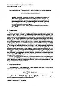
E, S and aS ¯ are plotted in Figure 5.1. It is obvious, that the set S is a PC-set. Furthermore, the set Zaf¯ is also a PC-set, which can be seen in Figure 5.2. The simulation is done for the Sparse Control case, i. e. ∀k ∈ N[0, M] : ut|k = u, ¯ with the initial time t0 = 0 ,

(5.16)

the initial value 10 x0 = 6

(5.17)

and the terminal time tf = 50 .

(5.18)

10

x2

5 0 −5 −10 −15

−10

−5

0 x1

5

10

15

Figure 5.1: Plot of the Mmax -step (A, B, K, W)-invariant set E (light gray), the εapproximation of the mPRI set of the considered dynamics S (dark gray) and the homothetic set aS ¯ (middle gray).

46

5.2 Example definition

10

x2

5

0

−5

−10 −15

−10

−5

0

5

10

15

Figure 5.2: Set Zaf¯ .

47


5.3 Simulations The simulations are done with MATLAB R2012a together with YALMIP [35], MultiParametric Toolbox 3.0 [36] and IBM ILOG CPLEX Optimization Studio. Due to numerical reasons, the simulation in this Thesis and in Brunner et al. [11, 24] are not completely equal. The inputs ut computed by Self-Triggered Tube MPC and Self-Triggered Homothetic Tube MPC are plotted in Figure 5.3, both in the sparse control case. Both methods lead to limit cycles due to the constant disturbance signals. See Khalil [18]. The comparison of the results shows, that Self-Triggered Homothetic Tube MPC leads to a smoother behavior of the input signals. This result has to be treated carefully. As the value function of the two methods are not identical and the choice of the maximal open-loop horizon ˆ t ) depends on the additive constant c, which was chosen arbitrarily to 50. Hence, the M(x results can not be compared reasonably. ˆ t ) calculated at the sampling time points tt are given for The open-loop horizons M(x i both cases in Figure 5.9. It is noticeable, that the open-loop horizon in the homothetic case reaches very fast the value 3 and holds. The value is never larger than 3, although Mmax = 5. The value of the open-loop horizon in the other case varies between 1 and 5 all the time. The average open-loop horizon for c = 50 is M¯ (T) = 2.84 and M¯ (HT) = 2.68, respectively. The average open-loop horizon for different values of the constant c is given in Table 5.1. By those results it is not possible to assess which scheme has the better performance with respect to the goal of maximizing the open-loop horizon. Furthermore, it is not clear how the behavior of the two methods would be in the case of another considered system. Therefore, the impact of the different parameters has to be examined systematically. But this would go beyond the boundaries of this diploma thesis. In Figure 5.5 the state constraint set X, an approximation of the region of attraction ˆ N=20 and the state trajectory xt of Self-Triggered Homothetic Tube MPC are plotted. X The comparison with Self-Triggered Tube MPC in Figure 5.4 shows, that the region of attraction is considerably larger in the Homothetic version. As expected, the adaptivity of the homothetic constraints sets compared to the conservative constraints sets of SelfTriggered Tube MPC leads to a larger region of attraction. Furthermore the two plots show, that in both cases sets are stabilized, not equilibrium points, and that in the SelfTriggered Homothetic Tube MPC case the trajectories converge nearer to a (theoretical) steady state (local origin of the stabilized set), that is not equal to the origin. Again there is no reasonable comparison possible as the size of the stabilized set depends on the constant c = 50. The reason for the offset is the considered constant disturbance signal. To steer the states to the origin (or another desired reference point in the state space), it is by the Internal Model Principle necessary that the structure of the disturbances have to be covered by the model of the controlled system. If this condition is not satisfied

48

5.3 Simulations

4 2 t

0 ut

5

10

15

20

25

30

35

40

45

50

−2 −4 stTMPC stHTMPC

−6 −8

Figure 5.3: Inputs ut computed by Self-Triggered Tube MPC (dashed line) and SelfTriggered Homothetic Tube MPC. Both in the sparse control case. by the original model, this could be done by disturbance estimation or by an extension of the states of the local controller σ by integrators. See Francis & Wonham [37] and Lunze [20]. In Figures 5.6 and 5.7 the value functions along the trajectories of the Self-Triggered Tube MPC case and the Self-Triggered Homothetic Tube MPC case are plotted, respectively. It is important to notice, that not a point in the state space is stabilized, but a set. Therefore the value functions don’t decrease to zero and hold, but they increase again. By the constraint in (3.23a), this increase is bounded by the value of the constant c, which can be seen in Figure 5.6 at time points t = 4 and t = 8. The average computational time per time step for the Self-Triggered Homothetic Tube MPC case and the Self-Triggered Tube MPC case are (HT) Tcomp. = 7.937s ,

(5.19)

(T) Tcomp.

(5.20)

= 0.616s ,

respectively. The values are calculated by dividing the overall simulation time by the total number of discrete time steps. As the software is not optimized for computational speed, these results have to be treated carefully. Most of the computational effort is spent for the translations of the constraints by YALMIP, not for the solving of the optimization problems.

49


10

x2

5

0

−5

−10

−20

−15

−10

−5

0 x1

5

10

15

20

Figure 5.4: State xt computed by Self-Triggered Tube MPC. The light gray set is the ˆ N=20 . state constraint set X. The dark gray set is the region of attraction X

10

x2

5

0

−5

−10

−20

−15

−10

−5

0 x1

5

10

15

20

Figure 5.5: State xt computed by Self-Triggered Homothetic Tube MPC. The light gray ˆ N=20 . set is the state constraint set X. The dark gray set is the region of attraction X

50

5.3 Simulations

500 450 400 350 VNM

300 250 200 150 100 50 0 0

5

10

15

20

25 t

30

35

40

45

50

Figure 5.6: Value function VNM along the trajectories of Self-Triggered Tube MPC and Self-Triggered Homothetic Tube MPC.

140 120

VNM

100 80 60 40 20 0 0

5

10

15

20

25 t

30

35

40

45

50

Figure 5.7: Value function VNM along the trajectories of Self-Triggered Homothetic Tube MPC.

51


6

VNM

5 4 3 2 1 0 0

5

10

15

20

25 t

30

35

40

45

50

40

45

50

Figure 5.8: Zoom of Figure 5.7.

5

ˆ t) M(x

4 3 2 1 0 0

5

10

15

20

25 t

30

35

ˆ t ) calculated at sampling time points tt for SelfFigure 5.9: Open-loop horizons M(x i Triggered Tube MPC (circles) and Self-Triggered Homothetic Tube MPC (triangles).

52

5.3 Simulations

c 0 1 10 20 50 100 1000

M¯ (T) 1.00 2.26 2.31 2.63 2.84 3.17 4.50

M¯ (HT) 1.00 2.38 2.68 2.68 2.68 2.94 2.94

Table 5.1: Average open-loop horizon M¯ for Self-Triggered Tube MPC (T) and SelfTriggered Homothetic Tube MPC (HT) for different constants c.

53

6 Conclusions and outlook In this chapter the main results are summarized and the conclusions are drawn. An outlook for possible further research is also presented.

6.1 Conclusions In this diploma thesis, a method of Self-Triggered Robust Model Predictive Control based on homothetic sets is introduced and compared with the method from Brunner et al. [11, 24], on which it is based. The difference between these methods lies in the construction of the sets, that describe the uncertainties in the states and inputs. While Self-Triggered Tube MPC uses conservatively large fixed sets depending on the maximal open-loop horizon (time between two control updates) M, Self-Triggered Homothetic Tube MPC uses adaptive sets, that are homothetic to offline-computed basic sets. The region of attraction of Self-Triggered Homothetic Tube MPC is considerably larger than that of Self-Triggered Tube MPC. On the other side, the computational effort and the complexity are higher. If the computational effort is no restriction, Self-Triggered Homothetic Tube MPC should be preferred. Otherwise Self-Triggered Tube MPC should be preferred. It is not clear which of the two schemes delivers in general the larger open-loop horizon.

6.2 Outlook In future investigations, it should be examined which of the two methods leads in general to a larger open-loop horizon. It should also examined, how big the impact of the different parameters on the open-loop horizon is. It is reasonable to spend more effort on handling multiplicative disturbances. The translation method, that is presented in Chapter 2, is very conservative and can lead to a large disturbance set W and therefore to a small region of attraction.

55

6 Conclusions and outlook

One research topic is the extension of Self-Triggered Homothetic Tube MPC to timevarying systems. For this purpose the stability has to be ensured by modified K -functions for time-varying systems. See Khalil [18] for details. Another open field is the extension to tracking and offset-free regulation of any equilibrium point at constant disturbances by disturbance estimation or integrator states. The most complex topic is the extension to nonlinear systems. In the nonlinear case, the MPC problem can not be a Quadratic Program (QP) any more, as the prediction constraint would be nonlinear. Additionally the constraint sets for the Tubes have to be constructed differently. The proofs in Chapter 4 have also be modified, as they base on linearity in various parts.

56

A Proof of Theorem 3 The proof of Theorem 3 is adopted from Brunner et al. [24]. It is identical to Theorem 2 with the only difference, that the set E is replaced by the set aS. ¯ Some parts have been repeated word-by-word. Proof. It holds that the value function JN in (3.20) is a convex function. Furthermore the set n o (x, d1N ) ∈ X ×D1N ) | d1N ∈ DN1 (x) (A.1) is convex. Hence, the value function VN1 in (3.21a) is a convex function on the feasible ˆ N . As the value function VN1 is bounded on X ˆ N , it follows by Rockafellar [38] that set X 1 ˆ N . Then VN is uniformly continuous on every compact set contained in the interior of X the fist part of Theorem 3 follows from Lemma 4 and Lemma 5. First it can be shown, that the cost function JN in (3.20) is a convex function. Consider ˆ N is convex. Furthermore consider that X ˆ N is contained in the that the feasible set n X o

projection of the set (x, d1N ) ∈ X ×D1N | d1N ∈ DN1 (x) onto Rn (the first n coordinates). ˆ N there exist d1N, 1 , d1N, 2 with VN1 (x1 ) = JN1 (d1N, 1 ) and This implies, that for any x1 , x2 ∈ X VN1 (x2 ) = JN1 (d1N, 2 ) such that n o (x1 , d1N, 1 ), (x2 , d1N, 2 ) ∈ (x, d1N ) ∈ X ×D1N | d1N ∈ DN1 (x) .

(A.2)

n o By the convexity of the set (x, d1N ) ∈ X ×D1N | d1N ∈ DN1 (x) , for any γ ∈ R[0, 1] it holds that (γ x1 + (1 − γ)x2 , γ d1N, 1 + (1 − γ)d1N, 2 ) n o ∈ (x, d1N ) ∈ X ×D1N | d1N ∈ DN1 (x)

(A.3)

and therefore

57

A Proof of Theorem 3 VN1 (γ x1 + (1 − γ)x2 ) ≤ JN1 (γ d1N, 1 + (1 − γ)d1N, 2 )

(A.4a)

≤ γ JN1 (γ d1N, 1 ) + (1 − γ)JN1 (d1N, 2 ) = γ VN1 (x1 ) + (1 − γ)VN1 (x2 )

(A.4b) (A.4c)

which completes the proof of the convexity of VN1 . Next the positive invariance of the Sc will be proven. For this purpose, consider two ˆ N , such that cases. In the fist case, consider xti ∈ X VN1 (xti ) ≤ α12 (α1−1 (c)) .

(A.5)

By Lemma 4 and Lemma 5, it holds that ∀ j ∈ N[1, M(x ˆ

ti )]

: VN1 (xti + j ) ≤ VN1 (xti ) − α1 (|xti |aS ¯ )+c

(A.6a)

≤ α12 (α1−1 (c)) − α1 (|xti |aS ¯ )+c

(A.6b)

≤ α12 (α1−1 (c)) + c

(A.6c)

,

such that xti + j ∈ Sc (compare with (4.81)). Consider next the second case with VN1 (xti ) > α12 (α1−1 (c)) .

(A.7)

By Lemma 4, it holds that 1 −1 α12 (|xti |aS ¯ ) ≥ VN (xti ) > α12 (α1 (c))

(A.8)

or equivalently −1 |xti |aS ¯ > α1 (c)

(A.9)

α1 (|xti |aS ¯ )>c .

(A.10)

and

Finally, by Lemma 5, it holds that ∀i ∈ N, ∀ j ∈ N[1, M(x ˆ

ti )]

:

VN1 (xti + j ) ≤ VN1 (xti ) − α1 (|xti |aS ¯ )+c ≤ VN1 (xti ) .

(A.11a) (A.11b)

Because of this decrease, together with (4.81) it holds that xti + j ∈ Sc if xti ∈ Sc . This implies, that the set Sc is positively invariant for the closed loop system under the control of the MPC feedback law.

58

Finally, the asymptotic stability will be proved. For this purpose, define the function o n (A.12) W (x) = max 0, VN1 (x) − (α12 (α1−1 (c)) + c) . By this definition, W is uniformly continuous on any compact set contained in the interior ˆ N , because VN1 has this property. Furthermore, W is bounded on X ˆ N . It holds that of X ∀x ∈ Sc : ˆ N \Sc : ∀x ∈ X

W (x) = 0 ,

(A.13a)

W (x) > 0 .

(A.13b)

ˆN Hence there exist the K -functions αW, 1 and αW, 2 , such that it holds for all x ∈ X αW, 1 (|x|Sc ) ≤ W (x) ≤ αW, 2 (|x|Sc ) .

(A.14)

See Brunner [33] for more details. By Lemma 4, Lemma 5, and the results above for the closed loop system it holds that ˆ ∀i ∈ N, ∀ j ∈ N[1, M(x ˆ )] , ∀xt0 ∈ XN : ti

W (xti + j ) ≤ W (xti ) .

(A.15)

This proves the stability of the set Sc for the closed-loop system. As next step, it will be shown, that the set Sc is attractive for all initial conditions in ˆ N . By Lemma 4, it holds that α12 (|x| ) ≥ VN1 (x) for all x ∈ X ˆ N . Hence, it holds that X aS ¯ n o ˆ N | α12 (|x| ) ≤ α12 (α1−1 (c)) + c (A.16a) Sc ⊇ x ∈ X aS ¯ n o −1 ˆ N | |x| ≤ α12 = x∈X (α12 (α1−1 (c)) + c) (A.16b) aS ¯ n o ˆ N | |x| ≤ α1−1 (c) =: Sˆ c . ⊇ x∈X (A.16c) aS ¯ Furthermore, it holds that n o ˆ N | ∃ e ∈ aS Sˆ c = x ∈ X ¯ : |x − e| ≤ α1−1 (c) n o ˆ N | ∃ e ∈ aS, = x∈X ¯ ∃ z ∈ Rn : x = z + e : |z| ≤ α1−1 (c) n o ˆ N ∩ z ∈ Rn | |z| ≤ α1−1 (c) ⊕ aS =X ¯ .

(A.17a) (A.17b) (A.17c)

ˆ N that By (A.16), it holds for all x ∈ X |x|Sc ≤ |x|Sˆ = c

min

(e, z): e∈aS ¯ |z|≤α1−1 (c)

|x − e − z| .

(A.18)

59

A Proof of Theorem 3 ˆ N and x ∈ In the following, consider only the case x ∈ X / Sc , such that it holds |x|Sˆ > 0 c and |x|aS > 0. It is obvious, that x − e = 6 0. Define the parametrization ¯ z :=

x−e f |x − e|

(A.19)

with f ∈ R and e ∈ aS ¯ ⊂ Rn . It is obvious that |z| = | f |. Furthermore, by |x|Sˆ > 0, it c

−1 ∗ follows that |x|aS ¯ > α1 (c). Therefore it holds that e 6= 0. Otherwise z = x − e with ∗ e = arg mine∈aS ¯ |x − e| would be feasible in (A.18). By that, it would hold that |x|Sˆ c = 0, which was excluded from the considered case. With this result, it follows that x − e |x|Sc ≤ |x|Sˆ ≤ min x − e − f (A.20a) c |x − e| (e, f ): e∈aS ¯ | f |≤α1−1 (c)

=

min

(e, f ): e∈aS ¯ | f |≤α1−1 (c)

=

min

|x − e| 1 −

f : | f |≤α1−1 (c)

|x|aS ¯ 1 −

1 f |x − e|

(A.20b)

f |x|aS ¯

(A.20c)

−1 = |x|aS ¯ − α1 (c) .

(A.20d)

f The line (A.20d) follows from the fact, that in order to minimize the difference 1 − |x−e| , f has to be positive and as large as possible and |x|aS ¯ has to be as small as possible. −1 As it holds that f ≤ α1−1 (c) (constraint in (A.20c)) and |x|aS ¯ > α1 (c), it follows that f |x−e| < 1.

With the definition of W in (A.12) and the positive invariance of the set Sc it can be inferred from Lemma 5 and (A.20), that for the closed-loop system (3.25) it holds ˆ ∀i ∈ N, ∀ j ∈ N[1, M(x ˆ )] , x0 ∈ XN that ti

n o W (xti + j ) ≤ max 0, W (xti ) − α1 (|xti |aS ¯ )+c n o ≤ max 0, W (xti ) − α1 (|xti |Sc + α1−1 (c)) + c n o = max 0, W (xti ) − αˆ W (|xti |Sc )

(A.21a) (A.21b) (A.21c)

with ∀s ≥ 0 :

60

αˆ W (s) := α1 (s + α1−1 (c)) − c .

(A.22)

As α1 is a K -function, it follows that αˆ W is also one. ˆ N is positive invariant for the closed-loop system and compact, by Because the set X (A.21) it follows that lim W (xti ) = 0 .

t →∞

(A.23)

ˆ N belongs to its region of attraction. Hence, the set Sc is asymptotically stable. The set X This completes the first part of the proof. For the second part of Theorem 3, consider VN1 (x) ≤ α12 (α1−1 (c)) + c. By Lemma 4 it follows that −1 −1 |x|aS ¯ ≤ α1 (α12 (α1 (c)) + c) ,

(A.24)

which leads to the second part of the assertion.

61

Bibliography

[1] J. Adamy, Nichtlineare Regelungen. Dordrecht: Springer, 2009. [2] D. Mayne, J. Rawlings, C. Rao, and P. Scokaert, “Constrained model predictive control: Stability and optimality,” Automatica, vol. 36, no. 6, pp. 789–814, 2000. [3] J. Rawlings and D. Mayne, Model Predictive Control: Theory and Design. Madison: Nob Hill Publishing, 2009. [4] L. Grüne and J. Pannek, Nonlinear Model Predictive Control. Berlin: Springer, 2011. [5] L. Chisci, J. Rossiter, and G. Zappa, “Systems with persistent disturbances: predictive control with restricted constraints,” Automatica, vol. 37, no. 7, p. 1019–1028, 2001. [6] D. Mayne, M. Seron, and S. Raković, “Robust model predictive control of constrained linear systems with bounded disturbances,” Automatica, vol. 41, no. 2, pp. 219–224, 2005. [7] S. Raković, B. Kouvaritakis, R. Findeisen, and M. Cannon, “Homothetic tube model predictive control,” Automatica, vol. 48, no. 8, pp. 1631–1638, 2012. [8] D. Bernardini and A. Bemporad, “Energy-aware robust model predictive control based on noisy wireless sensors,” Automatica, vol. 48, no. 1, pp. 36–44, 2012. [9] L. Feeney and M. Nilsson, “An Introduction to Event-triggered and Self-triggered Control,” in Twentieth Annual Joint Conference of the IEEE Computer and Communications Societies (INFOCOM). Anchorage, AK, USA, pp. 1548–1557, 2001. [10] W. Heemels, K. Johansson, and P. Tabuada, “An Introduction to Event-triggered and Self-triggered Control,” in 51st IEEE Conference on Decision and Control. Maui, Hawaii, USA, pp. 3270–3285, 2012. [11] F. Brunner, W. Heemels, and F. Allgöwer, “Robust Self-Triggered MPC for Constrained Linear Systems,” in European Control Conference (ECC) 2014. Strasbourg, France, pp. 472–477, 2014.

63

Bibliography

[12] E. Messerschmid and S. Fasoulas, Raumfahrtsysteme. Berlin Heidelberg: Springer, 3rd ed., 2009. [13] K.-Y. You and L.-H. Xie, “Survey of Recent Progress in Networked Control Systems,” Acta Automatica Sinica, vol. 39, no. 2, p. 101–117, 2013. [14] S. Boyd and L. Vandenberghe, Convex Optimization. Cambridge: Cambridge University Press, 15th ed., 2014. [15] M. Ulbrich and S. Ulbrich, Nichtlineare Optimierung. Basel: Birkhäuser, 2012. [16] C.-D. Munz and T. Westermann, Numerische Behandlung gewöhnlicher und partieller Differenzialgleichungen. Berlin: Springer, 2nd ed., 2009. [17] W. Dahmen and A. Reusken, Numerik für Ingenieure und Naturwissenschaftler. Berlin: Springer, 2nd ed., 2008. [18] H. Khalil, Nonlinear Systems. Upper Saddle River: Prentice Hall, 3rd ed., 2002. [19] J. Lunze, Regelungstechnik 1. Berlin: Springer, 7th ed., 2008. [20] J. Lunze, Regelungstechnik 2. Berlin: Springer, 6th ed., 2010. [21] S. Raković, E. Kerrigan, K. Kouramas, and D. Mayne, “Invariant Approximations of the Minimal Robust invariant Set,” IEEE Transactions on Automatic Control, vol. 50, no. 3, pp. 406–410, 2005. [22] R. Schneider, Covex Bodies: The Brunn-Minkowski Theory. Cambridge: Cambridge University Press, 1993. [23] F. Yang, Z. Wang, and Y. Hung, “Robust Kalman Filtering for Discrete TimeVarying Uncertain Systems With Multiplicative Noises,” IEEE Transactions on Automatic Control, vol. 47, no. 7, pp. 1179–1183, 2002. [24] F. Brunner, W. Heemels, and F. Allgöwer, “Extended unpublished version of [11] including proofs,” in European Control Conference (ECC) 2014. Strasbourg, France, pp. 472–477, 2014. [25] S. Raković, E. Kerrigan, K. Kouramas, and D. Mayne, “Invariant approximations of robustly positively invariant sets for constrained linear discrete-time systems subject to bounded disturbances,” Tech. Rep. CUED/F-INFENG/TR.473, Department of Engineering, University of Cambridge, 2004. [26] E. Gilbert and K. Tan, “Linear Systems with State and Control Constraints: The Theory and Application of Maximal Output Admissible Sets,” IEEE Transactions on Automatic Control, vol. 36, no. 9, pp. 1008–1020, 1991.

64

Bibliography

[27] I. Kolmanovsky and E. Gilbert, “Theory and Computation of Disturbance Invariant Sets for Discrete-Time Linear Systems,” Mathematical Problems in Engineering, vol. 4, pp. 317–367, 1991. [28] N. Bhatia and G. Szegö, Stability Theory of Dynamical Systems. Berlin: Springer, 1970. [29] R. Bellman, Dynamic Programming. Princeton: Princeton University Press, 1957. [30] M. Sniedovich, “A New Look at Bellman’s Principle of Optimality,” Journal of Optimization Theory and Applications, vol. 49, no. 1, pp. 161–176, 1986. [31] H. Chen and F. Allgöwer, “Constrained model predictive control: Stability and optimality,” Automatica, vol. 34, no. 10, pp. 1205–1217, 1998. [32] J. Barradas Berglind, T. Gommans, and W. Heemels, “Self-triggered MPC for constrained linear systems and quadratic costs,” in IFAC Conference on Nonlinear Model Predictive Control 2012. Noordwijkerhout, The Netherlands, pp. 342–348, 2012. [33] F. Brunner, “Lower and Upper K -function Bounds in Terms of Set-Distances,” tech. rep., University of Stuttgart, 2014. [34] M. Lazar, W. Heemels, S. Weiland, and A. Bemporad, “Stabilizing Model Predictive Control of Hybrid Systems,” IEEE Transactions on Automatic Control, vol. 51, no. 11, pp. 1813–1818, 2006. [35] J. Löfberg, “YALMIP : A toolbox for modeling and optimization in MATLAB,” in 2004 IEEE International Symposium on Computer Aided Control Systems Design. Taipei, Taiwan, pp. 284–289, 2004. [36] M. Herceg, M. Kvasnica, C. Jones, and M. Morari, “Multi-Parametric Toolbox 3.0,” in 2013 European Control Conference (ECC). Zürich, Switzerland, pp. 502–510, 2013. [37] B. Francis and W. Wonham, “The Internal Model Principle of Control Theory,” Automatica, vol. 12, no. 5, pp. 457–465, 1976. [38] R. Rockafellar, Convex Analysis. Princeton: Princeton University Press, 1970.

65

Eigenständigkeitserklärung Ich versichere hiermit, dass ich, Emre Aydiner, die vorliegende Diplomarbeit selbstständig angefertigt, abgesehen von der Mitwirkung der genannten Betreuer, keine anderen als die angegebenen Hilfsmittel benutzt und sowohl wörtliche, als auch sinngemäß entlehnte Stellen als solche kenntlich gemacht habe. Die Arbeit hat in gleicher oder ähnlicher Form noch keiner anderen Prüfungsbehörde vorgelegen. Weiterhin bestätige ich, dass das elektronische Exemplar mit den anderen Exemplaren übereinstimmt.

Ort, Datum

Unterschrift

67

Robust Self-Triggered Model Predictive Control for Discrete-Time ...

Robust Self-Triggered Model Predictive Control for Discrete-Time ...

Suggest Documents

Robust Model Predictive Control

Stability Constraints for Robust Model Predictive Control

Robust shrinking ellipsoid model predictive control for

Robust Multi-Model Predictive Control Using LMIs

Robust Constrained Model Predictive Control ... - Purdue Engineering

robust model predictive control under output constraints

Robust Constrained Model Predictive Control of Fast

Robust Time-Varying Model Predictive Control with

Robust Model Predictive Control Using Iterative

Robust Model Predictive Control via Scenario Optimization

Robust Adaptive Model Predictive Control of

A Linearized Robust Model Predictive Control Applied

Robust Model Predictive Control of Nonlinear Affine

Robust Distributed Model Predictive Control ...

Robust Temporal Logic Model Predictive Control

Robust Model Predictive Control for Non-Linear ... - ScholarlyCommons

A Robust Model Predictive Control Approach for Underwater Robotic ...

Robust Predictive Control using a GOBF Model for ...

Robust Online Model Predictive Control for a ... - IEEE Xplore

Practical Robust Linear Model Predictive Control for ... - Google Sites

Linear programming-based robust model predictive control for positive

Nonfragile Robust Model Predictive Control for Uncertain Constrained

Robust stability constraints for fuzzy model predictive control - Fuzzy

Robust feasibility in model predictive control - Control Group