ADMNSTR. DEFNS TECHL INFO CTR. ATTN DTIC-OCP (ELECTRONIC COPY). 8725 JOHN J KINGMAN RD STE 0944. FT BELVOIR VA 22060-6218. DARPA.
Discrimination of Objects Within Polarimetric Imagery Using Principal Component and Cluster Analysis by Melvin Felton, Kristan P. Gurton Daivd Ligon, and Adrienne Raglin
ARL-TR-4216
Approved for public release; distribution unlimited.
August 2007
NOTICES Disclaimers The findings in this report are not to be construed as an official Department of the Army position unless so designated by other authorized documents. Citation of manufacturer’s or trade names does not constitute an official endorsement or approval of the use thereof. Destroy this report when it is no longer needed. Do not return it to the originator.
Army Research Laboratory Adelphi, MD 20783-1197
ARL-TR-4216
August 2007
Discrimination of Objects Within Polarimetric Imagery Using Principal Component and Cluster Analysis Melvin Felton, Kristan P. Gurton David Ligon, and Adrienne Raglin Computational and Information Sciences Directorate, ARL
Approved for public release; distribution unlimited.
Form Approved OMB No. 0704-0188
REPORT DOCUMENTATION PAGE
Public reporting burden for this collection of information is estimated to average 1 hour per response, including the time for reviewing instructions, searching existing data sources, gathering and maintaining the data needed, and completing and reviewing the collection information. Send comments regarding this burden estimate or any other aspect of this collection of information, including suggestions for reducing the burden, to Department of Defense, Washington Headquarters Services, Directorate for Information Operations and Reports (0704-0188), 1215 Jefferson Davis Highway, Suite 1204, Arlington, VA 22202-4302. Respondents should be aware that notwithstanding any other provision of law, no person shall be subject to any penalty for failing to comply with a collection of information if it does not display a currently valid OMB control number.
PLEASE DO NOT RETURN YOUR FORM TO THE ABOVE ADDRESS. 1. REPORT DATE (DD-MM-YYYY)
2. REPORT TYPE
3. DATES COVERED (From - To)
August 2007
Final
January to May 2007
4. TITLE AND SUBTITLE
5a. CONTRACT NUMBER
Discrimination of Objects Within Polarimetric Imagery Using Principal Component and Cluster Analysis
5b. GRANT NUMBER
5c. PROGRAM ELEMENT NUMBER
6. AUTHOR(S)
5d. PROJECT NUMBER
Melvin Felton, Kristan P. Gurton, David Ligon, and Adrienne Raglin 5e. TASK NUMBER
5f. WORK UNIT NUMBER
8. PERFORMING ORGANIZATION
7. PERFORMING ORGANIZATION NAME(S) AND ADDRESS(ES)
REPORT NUMBER
U.S. Army Research Laboratory ATTN: AMSRD-ARL-CI-ES 2800 Powder Mill Road Adelphi, MD 20783-1197
ARL-TR-4216
9. SPONSORING/MONITORING AGENCY NAME(S) AND ADDRESS(ES)
10. SPONSOR/MONITOR'S ACRONYM(S)
U.S. Army Research Laboratory 2800 Powder Mill Road Adelphi, MD 20783-1197
11. SPONSOR/MONITOR'S REPORT NUMBER(S)
12. DISTRIBUTION/AVAILABILITY STATEMENT
Approved for pubic release; distribution unlimited. 13. SUPPLEMENTARY NOTES
14. ABSTRACT
We apply two multivariate image analysis techniques to several sets of spatially coincident, long-wave infrared (LWIR), polarimetric images to improve target contrast and/or aid in the identification of certain object features not present in the original image set. Principal component analysis (PCA) was used to obtain new representations of the scene that highlight target features based upon the variance of the variables used in the analysis. We show a representation of the scene that maintains the same level of target-to-background contrast (when compared to the conventional thermal and degree of linear polarization images), as well as additional information content contained in the resultant PCA analysis. Cluster analysis (CA) was used to group pixels of the image that have similar values for the variables chosen. We show that this method is an effective means for separating objects of interest from complex backgrounds, as well as subdividing different features of an object. 15. SUBJECT TERMS
Principal component analysis, cluster analysis, polarimetric, thermal imagery, image processing 17. LIMITATION OF ABSTRACT
16. Security Classification of: a. REPORT
b. ABSTRACT
c. THIS PAGE
Unclassified
Unclassified
Unclassified
U
18. NUMBER OF PAGES
31
19a. NAME OF RESPONSIBLE PERSON
Melvin Felton 19b. TELEPHONE NUMBER (Include area code)
(301) 394-2618 Standard Form 298 (Rev. 8/98) Prescribed by ANSI Std. Z39.18
ii
Contents
List of Figures
iv
List of Tables
v
Introduction
1
LWIR Polarimetric Imagery
3
Image Processing Method
5
Principle Component Analysis (PCA)
5
Cluster Analysis (CA)
6
Results
7
Discussion
18
References
20
Distribution List
21
iii
List of Figures Figure 1. Image a. and b. show a conventional visible and LWIR thermal image, respectively, of a vehicle parked in a tree-line and obscured from view. Image c. shows a resultant polarimetric image (commonly termed an S1 image), that is a measure of vertically polarized radiation compared to horizontally polarized radiation. Black regions within the binary image c. signify regions where the difference between the vertical and horizontal sates is zero. The colored region(s) signify some finite difference implying a man-made object is present. Image d. shows image b. and c. being fused together highlighting the presence of a hidden vehicle............................................................................2 Figure 2. The LWIR polarimetric imager is designed to produce well calibrated polarimetric and/or Stokes imagery................................................................................................................5 Figure 3. Visible image of scene 1, which is a vehicle in the brush...............................................8 Figure 4. LWIR DOLP 30x30 pixel image of the vehicle in scene 1.............................................8 Figure 5a. First derived image which accounts for nearly half of the variance in the data cube of scene 1 and is dominated by DOLP and ORT.....................................................................10 Figure 5b. Second derived image which accounts for nearly 40% of the variance in the data cube of scene 1 and is dominated by S0...................................................................................10 Figure 5c. Third derived image which accounts for approx. 14% of the variance in the data cube of scene 1. The magnitudes of the eigenvector components are more evenly distributed. ...............................................................................................................................11 Figure 6a. Cluster analysis plot for 19 clusters. The background is comprised of clusters 1 through 3 while the features of the vehicle are classified between clusters 4 through 19.......12 Figure 6b. Cluster analysis plot for 11 clusters. Clusters 1 through 3 are predominantly the background but do consist of some portions of the vehicle. Clusters 4 through 11 correspond to the vehicle. ........................................................................................................12 Figure 6c. Cluster plot for 2 clusters. Cluster 1 is predominantly the background but does contain some of the vehicle. Cluster 2 consists mainly of the side of the vehicle.................13 Figure 7. Visible image of scene 2 which is a mobile rocket launcher in the brush.....................13 Figure 8. LWIR DOLP 30x30 pixel image of mobile rocket launcher in scene 2. ......................14 Figure 9a. First derived image which accounts for 44% of the variance of the data cube of scene 2 and is dominated by DOLP and S0..............................................................................15 Figure 9b. Second derived image which accounts for 33% of the variance of the data cube in scene 2 and is dominated by ORT. ..........................................................................................16 Figure 9c. Third derived image which accounts for 23% of the variance of the data cube in scene 2 and is dominated by DOLP and S0..............................................................................16 Figure 10a. Cluster plot for 15 clusters. Clusters 1 through 7 corresponds to the background while 8 through 15 to the mobile rocket launcher. ..................................................................17
iv
Figure 10b. Cluster plot for 5 clusters. Clusters 1 and 2 correspond to the background and 3 through 5 correspond to the mobile rocket launcher. ..............................................................17 Figure 10c. Cluster plot for 3 clusters. Cluster 1 corresponds to the background and clusters 2 and 3 correspond to the mobile rocket launcher. ..................................................................18 Figure 10d. Cluster plot for 2 clusters. Cluster 1 corresponds to the background and rocket and cluster 2 to the vehicle and mount of the rocket launcher.................................................18
List of Tables Table 1. Percent variance and cumulative percent variance for the principal components. ...........8 Table 2. Components of the eigenvectors Vi (i=1,2,3) which serve as basis vectors for the projection of the data in the multivariate space of scene 1. .......................................................9 Table 3. Percent variance and cumulative percent variance for the principal components. .........14 Table 4. Components of the eigenvectors Vi (i=1,2,3) which serve as basis vectors for the projection of the data in the multivariate space of scene 2. .....................................................14
v
INTENTIONALLY LEFT BLANK
vi
Introduction There is great interest in assessing the usefulness of polarization-based imaging for improved targeting and tracking of “man-made” objects that are obscured by complex “natural” backgrounds (1). Polarimetric based imaging shows particular promise when applied in the thermal infrared (IR) (2). Thermal IR polarimetric imaging exploits the fact that man-made objects, such as vehicles, roads, buildings, etc., tend to emit radiation that exhibits a greater degree of polarization than natural background materials i.e., soil, vegetation, brush, etc. By filtering the image forming radiation based solely on polarization state, one can construct a polarimetric image that highlights objects that are most polarized and suppress regions of the scene that are least polarized. The net result is that thermal polarimetric imagery tends to increase the contrast between the man-made targets and complex backgrounds within a scene. In a study by Gurton et al., it has been shown that information content is greatly enhanced by fusing polarimetric imagery with conventional thermal imagery (1). An example of this can be seen in figures (1a through 1d.).
1
a.
b.
c.
d.
Figure 1. Image a. and b. show a conventional visible and LWIR thermal image, respectively, of a vehicle parked in a tree-line and obscured from view. Image c. shows a resultant polarimetric image (commonly termed an S1 image), that is a measure of vertically polarized radiation compared to horizontally polarized radiation. Black regions within the binary image c. signify regions where the difference between the vertical and horizontal sates is zero. The colored region(s) signify some finite difference implying a man-made object is present. Image d. shows image b. and c. being fused together highlighting the presence of a hidden vehicle.
However, because polarimetric imaging produces a multivariate set of at least four spatially coincident images per frame, i.e., thermal intensity, amount of horizontally and vertically polarized light, amount of +45°and –45° polarized light, and the amount of left- and rightcircular polarized light, there are many ways of processing the data to identify objects of interest. As a result, polarimetry (as well as multi- or hyper-spectral imaging) generates a significant sized data cube that must be processed in real-time (or pseudo-realtime) rates. Therefore, it is desirable to work with a reduced data set to increase computational efficiencies. Several image processing techniques have been suggested that would produce a reduced data set for analysis and provide varying degrees of image enhancement.
2
Sadjadi, et al., presented a suite of algorithms designed for automatic target recognition (ATR) and detection within IR polarimetric imagery (3,4). The algorithms were tested using simulated IR polarimetric imagery and required an estimate of the size of the object of interest in terms of its pixel area within the scene, as well as an a priori generated library of first and second order statistics for the particular object being examined. Zallat, et al., proposed methods based on cluster analysis that involves polarization enhancement and an image processing algorithm based on a Markovian model (5). We propose applying a well-known multivariate image processing technique called principal component analysis (PCA) that reduces the overall data set, and then apply a cluster analysis (CA) methodology to increase processing efficiency further (6). We applied these techniques to various polarimetric image cubes of recorded long-wave infrared (LWIR) polarimetric imagery of DoD relevant targets recorded during various field tests during the summer of 2006. First, we describe the polarimetric data acquisition methodology and the LWIR polarimetric imager used to record the polarimetric images used here. We then describe in detail the particular features unique to the PCA and CA methods used in this study and present examples of processed imagery. Finally, we end with a discussion highlighting the various strengths and weaknesses associated with either PCA or CA and suggest conditions for optimum utility.
LWIR Polarimetric Imagery The polarimetric camera system used is a modified LWIR thermal imager designed to produce well calibrated Stokes imagery by deriving the Stokes parameters over the wavelength region 8.5 to 10.5 μm. The Stokes parameters are then used to calculate the degree of linear polarization (DOLP) and an orientation angle (ORT). The definitions of the Stokes images as well as the DOLP and ORT images are defined by equations 1 through 6,
S 0 ≥ S12 + S 22 + S 32 ,
(1)
S1 = I (0) − I (90) ,
(2)
S 2 = I (+ 45) − I (− 45),
(3)
S 3 = I (R ) − I (L ),
(4)
DOLP = S12 + S 22 S 0 ,
(5)
ORT = 1 2(arctan(S1 S 2 ))
(6)
and
3
where I(0), I(90), and I(±45) represent the measured radiance values obtained when a polarizer placed in front of a detector is rotated through 0°, 90°, and ±45° with respect to the observation plane and I(R) and I(L) represent the right- and left-handed circular states. Here we define the observation plane as the plane that contains the surface normal at a point on an object and the line-of-sight vector from the camera to that point on the object. Notice that S0 is simply the incident irradiance and that the equality holds for completely polarized light. S1, S2, and S3 specify the state of polarization. From equation 2, we see that if S1 > 0, there is an abundance of horizontal polarization, and if S1 < 0 there is an abundance of vertical polarization. If S1 = 0 there is no preferential polarization with respect to the horizontal or the vertical. Similarly, in equation 3 if S2 > 0 there is an abundance of +45° polarization and if S2 < 0, there is an abundance of –45° polarization. The LWIR polarimetric imager consists of two primary components: 1) a polarimetric module that houses a spinning achromatic cadmium selenide (CdSe) quarter wave plate which is mounted in series with a fixed wire-grid polarizer, and 2) a camera module that consists of a liquid nitrogen cooled, 240x360 pixel, mercury cadmium telluride (MCT) focalplane-array (FPA) (see figure 2). Sequential LWIR polarimetric images are recorded digitally at a rate as fast as 240 frames/sec and synchronized to the rotation of the spinning CdSe wave-plate. The spinning wave-plate and fixed wire-grid polarizer combination effectively acts like a variable polarimetric filter. As a result, each digital image recorded is generated by polarized emittance of a particular orientation. Although the maximum acquisition rate is 240 frames/second, the present data were acquired at 128 frames/second and the 240x360 pixels FPA was windowed down to 152x158 pixels. With the speed of the spinning wave plate set at 8 revolutions/second, 16 frames were measured every 125 ms and averaged over 10 revolutions. The averaged frames were then used with a prerecorded calibration file to derive the four Stokes images. The imager was calibrated by recording the radiometric response when we observe known linear polarization states produced by the transmission of the radiance from an extended blackbody through a wire-grid polarizer, allowing us to measure the intensity parameters in equations 2 and 3. Because in practice we have seen no evidence of circularly polarized emission in the natural environment, the corresponding Stokes image S3 (equation 4) is always taken to be zero in this analysis. Therefore, we did not measure I(L) or I(R) in the calibration procedure.
4
Figure 2. The LWIR polarimetric imager is designed to produce well calibrated polarimetric and/or Stokes imagery.
Image Processing Method For static or slowly moving objects the LWIR polarimetric imager generally produces a minimum of 4 multivariate Stokes images as described above. This results in a stack of images in which the pixel positions match for all of the images in the stack (6). For the analysis conducted here, we considered only the most robust Stokes image(s) and polarimetric products, i.e., the three values DOLP, ORT, and S0. We then apply PCA and CA to a given stack of three images, which serve to characterize the scene. The first step is to construct a data matrix, X np , from a given image stack such that the n row(s) represent the pixels of a particular image in the stack, and the p column(s) are taken to be a particular variable associated with one of the multivariate images, e.g., p represents one of the 3 parameters defining our image stack, DOLP, ORT, or S0. This creates a p-dimensional variable space in which each pixel is represented by a p-element vector which allows the similarities of the pixels to be assessed geometrically (5). If the image stack used is 30x30 = 900 pixels, then n = 900. Since our image space is limited to the 3 states DOLP, ORT, and S0, p=3. Therefore the dimensions for the data matrix, X np , produced from a typical image stack is 900 x 3.
Principle Component Analysis (PCA) PCA was used to obtain a reduced/alternative representation of the image stack which effectively performs a linear transformation that projects the data set to a new orthogonal multi-dimension coordinate system, thus creating a new set of derived variables. This projection is such that the 5
greatest variance of the data lies on the first coordinate, the second greatest variance on the second coordinate, and so on. By displaying the image of each derived variable, we obtain a representation of the original image in terms of the interrelationships between the variables in the data set (7). We begin by calculating the covariance matrix, C np , of the standardized data matrix, S np . The data, X np , was standardized to avoid dominance of one variable over another by dividing each element by its corresponding column-wise variance, σp. S np = X np σ p
(7)
The eigenvectors and eigenvalues of C np were calculated and placed in descending order according to the eigenvalues to obtain Vpp and λp, respectively. The projection into variable space, Pnp, is obtained by the matrix multiplication in equation 8. Pnp = C np ⋅ V pp
(8)
The matrix Pnp consists of derived variables that are the projection of the original data set onto the basis found in the PCA. The image plot of Pnp reflects the correlation of each pixel with the principal components. Examination of the elements of Vpp reveals detailed information of the contribution of each variable to the principal components. Other meaningful parameters include the “percent energy” which is obtained by calculating the cumulative sum of the elements of λp. The percent energy represents the amount of the variance of the entire data set that is accounted for based upon the number of principal components one chooses to include in the analysis. This also allows for the reduction of the dimensions of the data by disregarding the principal components that only account for a negligible amount of the total variance.
Cluster Analysis (CA) CA was used to exploit the tendency for distinct objects and/or regions of objects to have similar values for all p variables in the variable space (7). A geometrical distance in the p-dimensional variable space can be used to determine the similarity between pixels. A Euclidean distance metric, given by equation 9 was used in this analysis. An n × n matrix was calculated (where n is the number of pixels) whose elements are the distances between each pixel in the p-dimensional variable space. d ij =
(x
− x j1 ) + (xi 2 − x j 2 ) + " + (xip − x jp ) , 2
i1
2
6
2
i,j≤ n
(9)
The cluster algorithm used in this analysis was agglomerative and hierarchical, i.e., each pixel begins as an individual cluster, and as the algorithm progresses, the two clusters that are closest are fused until the only remaining cluster contains all of the pixels of the image. In addition, once a pixel is placed in a cluster, it remains in it through the termination of the algorithm. Each time a cluster acquires a new member (pixel), its distance in the p-dimensional variable space with respect to the remaining clusters must be recalculated. In this study, the distance between two clusters containing more than one pixel is defined as the average distance between all of the members of each cluster, known as average-linkage. To limit computation times, we performed the analysis on subsections of the original LWIR imagery that we feel contain objects of interest.
Results The results presented here will consist of two scenes that each contains an object of interest. The geometry of the objects of interest in the scenes differs greatly from each other, allowing for an assessment of the robustness of the algorithm’s ability to distinguish the objects from the background as well as distinguish various features of the object. For each scene a visible and DOLP image are presented for comparison followed by the PCA and CA results. The PCA results consist of the cumulative percent energy, eigenvectors, and principal component plots. The CA results consist of cluster plots that exemplify the evolution of the clustering processes. The data was grouped into a range of 2 to 20 clusters. The images that best exemplify the progression of the cluster output were selected for presentation below. Scene 1 The first scene is shown in figure 3 for reference and consists of a vehicle that is in the brush. A corresponding LWIR DOLP image is shown in figure 4 (the highly pixilated nature of the polarimetric image is due to the fact that it is a subsection of the original image, i.e. the original image is 152x158 pixels, and figure 4 is only a 30x30 pixel subsection of the original).
7
Figure 3. Visible image of scene 1, which is a vehicle in the brush.
Figure 4. LWIR DOLP 30x30 pixel image of the vehicle in scene 1.
The percent variance and cumulative percent variance for the three principal components are shown in table 1. The first component accounts for the largest amount of the variance, approximately 48%. The next component accounts for 38% and the last for 14%. The components of the eigenvectors listed in table 2 indicate each variable’s contribution to the principal components. Table 1. Percent variance and cumulative percent variance for the principal components. Principal Component 1 2 3
Percent Variance 48 38 14
8
Cum. Percent Variance 48 86 100
Table 2.
DOLP ORT S0
Components of the eigenvectors Vi (i=1,2,3) which serve as basis vectors for the projection of the data in the multivariate space of scene 1. V2 –0.40393 0.21718 0.88864
V1 0.67202 0.72953 0.12717
V3 0.62067 –0.64855 0.44063
The variables that contribute most to the first principal component are DOLP and ORT. Recall that, from table 1, the first principal component accounts for nearly half of the variance within the data set. This suggests that thermal intensity, S0, does not contain the important information within the scene, i.e., there is low thermal contrast. In addition, note that each variable is directly correlated to each other in the first component. On the other hand, the second principal component is dominated by S0 and DOLP is now inversely correlated with ORT and S0. The contribution to the third principal component is distributed more evenly among the variables in the data set than for the first two principal components and ORT is inversely correlated to DOLP and S0. Figures 5a-c show the principle component images listed in descending order. These images contain the information about the correlations of each variable with respect to each principal component. One can see in figure 5a the lighter colored pixels are directly correlated to the first principal component which, as we saw in table 2, is dominated by both DOLP and ORT whose eigenvector component magnitudes are 0.67202 and 0.72953, respectively. The darker pixels are inversely correlated to the first principal component. Also, note that there is good contrast between the vehicle and the background. Because the contribution by S0 to the first derived variable is so low, this also suggests that there is low thermal contrast within this scene. However, figure 5b shows that the same region of pixels is directly correlated to the second principal component which is dominated by the total radiance image, S0 (see table 2). Note that this corresponds to a decrease in the amount of contrast between the vehicle and the background in figure 5b. The interpretation of figure 5c is more difficult because, as can be seen in table 2, the magnitudes of the components of the eigenvectors are much closer and less distinct, and as a result the third principal component accounts for the smallest percent of the total variance seen in the image.
9
Figure 5a. First derived image which accounts for nearly half of the variance in the data cube of scene 1 and is dominated by DOLP and ORT.
Figure 5b. Second derived image which accounts for nearly 40% of the variance in the data cube of scene 1 and is dominated by S0.
10
Figure 5c. Third derived image which accounts for approx. 14% of the variance in the data cube of scene 1. The magnitudes of the eigenvector components are more evenly distributed.
Figures 6a-c are cluster plots that exemplify the progression of the clustering output. The color bar corresponds to the cluster number. Figure 6a shows the scene classified into 19 clusters. The background is comprised of clusters 1 through 3 while the features of the vehicle are classified between clusters 4 through 19. Clusters 16 through 19 represent the front of the vehicle, while the rest of the vehicle is generated via clusters 4 through 15. In figure 6b, the scene is split into 11 clusters. Most of the original background has now been fused into one cluster. Also fused into this “background” cluster are some pixels that correspond to the vehicle, mainly its wheels. Other clusters that represented portions of the vehicle in the previous calculation have been fused together as well. In figure 6c, the scene is now split into only two clusters. All of the background has become one homogeneous cluster. Also included in this cluster are portions of the vehicle which mainly include the front and wheels. Therefore, the two distinct clusters that remain are the background and the side of the vehicle.
11
Figure 6a. Cluster analysis plot for 19 clusters. The background is comprised of clusters 1 through 3 while the features of the vehicle are classified between clusters 4 through 19.
Figure 6b. Cluster analysis plot for 11 clusters. Clusters 1 through 3 are predominantly the background but do consist of some portions of the vehicle. Clusters 4 through 11 correspond to the vehicle.
12
Figure 6c. Cluster plot for 2 clusters. Cluster 1 is predominantly the background but does contain some of the vehicle. Cluster 2 consists mainly of the side of the vehicle.
Scene 2 The second scene, shown in figure 7, is of a mobile rocket launcher located in the brush. The DOLP image is shown in figure 8. Notice that the geometry of this vehicle is very different from the vehicle in scene 1 (figure 3).
Figure 7. Visible image of scene 2 which is a mobile rocket launcher in the brush.
13
Figure 8. LWIR DOLP 30x30 pixel image of mobile rocket launcher in scene 2.
The percent variance and cumulative percent variance for the three principal components is shown in table 3. Of the three principal components, the first accounts for the largest amount of the variance, approximately 44%. The last two principal components account for 33% and 23% of the variance, respectively. The 3 components of the eigenvectors are listed in table 4. The variables that contribute most to the first principal component are DOLP and S0 images and DOLP and ORT are inversely correlated to S0. As opposed to scene 1, S0 is important in scene 2 because the shadowed (i.e., cool) regions are very prominent. The second principal component is dominated by ORT and DOLP is now inversely correlated to ORT and S0. The contribution to the third principal component is dominated by DOLP and S0, respectively, and all of the variables are directly correlated. Table 3. Percent variance and cumulative percent variance for the principal components. Principal Component 1 2 3
Table 4.
DOLP ORT S0
Percent Variance 44 33 23
Cum. Percent Variance 44 77 100
Components of the eigenvectors Vi (i=1,2,3) which serve as basis vectors for the projection of the data in the multivariate space of scene 2. V2 0.20562 -0.97824 -0.02758
V1 -0.69008 -0.16492 0.70469
14
V3 0.69391 0.12586 0.70898
Figures 9a-c are the 1st, 2nd, and 3rd derived images for the scene shown in figure 8. The dark and light pixels are negatively and positively correlated, respectively, to the first principal component shown in figure 9a. Recall that the first principal component is dominated by DOLP and S0, whose eigenvector component magnitudes are 0.69008 and 0.70469, respectively (see table 4). It is apparent that the dark pixels in figure 9a correspond to the rocket, while the light pixels correspond to the side of the vehicle transporting the rocket. In figure 9b, the pixels that are positively correlated to the second principal component, which is dominated by ORT (see table 4), seem to correspond to the side of the vehicle as well as the rocket mount. Note that in the portion of figure 9b that corresponds to the vehicle, a portion of the back of the vehicle is inversely correlated to the second principal component, while the side of the vehicle is positively correlated. This is consistent with the fact that the second principal component is dominated by ORT. However, figure 9c shows that the pixels corresponding to the rocket are positively correlated to the third principal component (which, as seen in table 4, is dominated by DOLP and S0).
Figure 9a. First derived image which accounts for 44% of the variance of the data cube of scene 2 and is dominated by DOLP and S0.
15
Figure 9b. Second derived image which accounts for 33% of the variance of the data cube in scene 2 and is dominated by ORT.
Figure 9c. Third derived image which accounts for 23% of the variance of the data cube in scene 2 and is dominated by DOLP and S0.
Figures 10a-d are the cluster plots for scene 2. Figure 10a shows the scene classified into 15 clusters. Clusters 1 through 7 corresponds to the background while 8 through 15 to the mobile rocket launcher. In figure 10b, many of clusters have been combined so that there are only five clusters. The first two clusters correspond to the background, while the rest correspond to the mobile rocket launcher.
16
Specifically, cluster 3 is the side of the vehicle and the rocket mount, and cluster 4 the rocket, and cluster 5 is a solitary pixel that corresponds to the side of the vehicle. Figure 10c shows that the number of clusters have been reduced further, to three. Here the background is represented homogeneously by cluster 1, the rocket by cluster 2, and the side of the vehicle and rocket mount by cluster 3. Finally, shown in figure 10d one can see that the rocket has been combined with the background so that the only remaining clusters are the background and the side of the vehicle along with the rocket mount.
Figure 10a. Cluster plot for 15 clusters. Clusters 1 through 7 corresponds to the background while 8 through 15 to the mobile rocket launcher.
Figure 10b. Cluster plot for 5 clusters. Clusters 1 and 2 correspond to the background and 3 through 5 correspond to the mobile rocket launcher.
17
Figure 10c. Cluster plot for 3 clusters. Cluster 1 corresponds to the background and clusters 2 and 3 correspond to the mobile rocket launcher.
Figure 10d. Cluster plot for 2 clusters. Cluster 1 corresponds to the background and rocket and cluster 2 to the vehicle and mount of the rocket launcher.
Discussion The utility for applying PCA to multivariate polarimetric images is demonstrated by processing subsections of two polarimetric images that each contains an object of interest. The original DOLP image regions seen in figures 4 and 8 were intentionally chosen to test how effective the 18
PCA methodology is for enhancing original imagery when applied to a simple three channel polarimetric image cube. As seen in the resultant first component images (or “derived” image) shown in 5a and 9a, information concerning all of the variables used in the analysis has been incorporated into an image that maintains the same level of contrast and target features as the original DOLP images. Thus, the PCA methodology provides a more efficient means for analyzing the relationships of the variables in the data set. We have used the fact that principle components contain the information of the data set in descending order to isolate the useful information for further analysis. In general, the first component images have the least amount of “noise” because they contain small contributions of the channels with the smallest amount of contrast. The later components get noisier since they contain less of the total sum of the squares when compared to the first component image, i.e., they contain more of the channels with the smallest amount of contrast. As mentioned earlier, the first score images seen in either figures 5a or 9a represents a weighted average of the most intense raw image of the polarimetric image cube (sometimes termed a “stack”). These images can be considered as a noise-reduced “mean” image. In many other applications, the first component score image plays an analogous role as a noise-reduced mean. The score images seen in figures 5 and 9 shows additional detail of the sample and may be of use depending on the application. Because the principal components are orthogonal, the corresponding score images show optimal visual contrast between two consecutive scores, i.e., most noticeable between the first and second score images. The net effect of this is to enhance target features not visible in any single image of the original multivariate image set. This additional information may be useful in identifying objects not readily distinguishable from complex backgrounds. In addition, we also apply cluster analysis that takes into account the similarity (or dissimilarity) of all the variables for each data point to provide a representation of the objects within a scene. When the number of clusters that a scene is split into is large, the algorithm attempts to distinguish between different features of the same object, i.e., one object may be split into more than one cluster. A limitation of the technique is that the ability of the algorithm to provide information about the features of a particular object depends upon the size of the object within the field-of-view of the camera. If the object is large within the field of view, then the clusters may reveal information about the geometrical shape and orientation of the object. If the object is small within the field of view, the algorithm will most likely have trouble accurately representing the different features of the object. A detailed study of the mean polarimetric values for each cluster will have to be performed to understand its ability to represent various features of objects. Another limitation of this technique is that it is computationally extensive. The array sizes involved can become very large, thus slowing the run-time of the algorithm. To improve upon the technique, it is recommended that the multivariate image analysis be made more efficient to improve the run-time for large subsections of polarimetric images. In addition, this algorithm should be combined with another algorithm that quickly identifies locations, or subsections, within the entire image that the multivariate image analysis can then be applied to.
19
References 1. Gurton, Kristan P.; Dahmani, R.; Videen G. Effect of surface roughness and complex indices of refraction on polarized thermal emission. Appl. Opt. 2005, 44, 36. 2. Gurton, Kristan P. Advancement in Polarimetric Sensor Design, Military Sensing Symposium (MSS) Polarimetric Workshop, Atlanta, GA, 4–6 December 2006. 3. Sadjadi, F.; Chun, C. Improved Feature Classification by means of a Polarimetric IR Imaging Sensor. IEEE 1996, 396–398. 4. Sadjadi, F. Polarimetric IR Automatic Target Detection and Recognition. IEEE 1996, 2140–2143. 5. Zallat, J. Clustering of polarization-encoded images. Appl. Opt. 2004, 43 (2), 283–292. 6. Geladi P.; Grahn, H. Multivariate Image Analysis. John Wiley & Sons Inc., 1996. 7. Dillon, W.; Goldstein, M. Multivariate Analysis: Methods and Applications. John Wiley & Sons Inc., 1984.
20
Distribution List ADMNSTR DEFNS TECHL INFO CTR ATTN DTIC-OCP (ELECTRONIC COPY) 8725 JOHN J KINGMAN RD STE 0944 FT BELVOIR VA 22060-6218
US ARMY AVIATION & MIS LAB ATTN AMSRD-AMR-SG-IP H F ANDERSON BLDG 5400 REDSTONE ARSENAL AL 35809
DARPA ATTN IXO S WELBY 3701 N FAIRFAX DR ARLINGTON VA 22203-1714
US ARMY CECOM RDEC NVESD ATTN J HOWE 10221 BURBECH RD STE 430 FT BELVOIR VA 22060-5806
OFC OF THE SECY OF DEFNS ATTN ODDRE (R&AT) THE PENTAGON WASHINGTON DC 20301-3080
US ARMY INFO SYS ENGRG CMND ATTN AMSEL-IE-TD F JENIA FT HUACHUCA AZ 85613-5300 US ARMY NVESD ATTN AMSRD-CER-NV-ST-ICT M A SCHATTEN 10221 BURBECK RD FT BELVOIR VA 22060-5806
ADVANCED TECHNOLOGIES DIRECTORATE SPACE & MISSILE COMMAND ATTN D LIANOS PO BOX 1500 HUNTSVILLE AL 35805
COMMANDER US ARMY RDECOM ATTN AMSRD-AMR W C MCCORKLE 5400 FOWLER RD REDSTONE ARSENAL AL 35898-5000
US ARMY TRADOC BATTLE LAB INTEGRATION & TECHL DIRCTRT ATTN ATCD-B 10 WHISTLER LANE FT MONROE VA 23651-5850
US ARMY RSRCH LAB ATTN AMSRD-ARL-CI-OK-TP TECHL LIB T LANDFRIED BLDG 4600 ABERDEEN PROVING GROUND MD 21005-5066
SMC/GPA 2420 VELA WAY STE 1866 EL SEGUNDO CA 90245-4659
AIR FORCE RSRCH LAB AFRL/MNGG ATTN D R SNYDER 101 WEST EGLIN BLVD EGLIN AFB FL 32542-6810
US ARMY ABERDEEN TEST CENTER ATTN CSTE-DT-AT-WC-A F CARLEN 400 COLLERAN ROAD ABERDEEN PROVING GROUND MD 21005-5009
21
US GOVERNMENT PRINT OFF DEPOSITORY RECEIVING SECTION ATTN MAIL STOP IDAD J TATE 732 NORTH CAPITOL ST., NW WASHINGTON DC 20402 ARROW PROGRAM OFFIC ATTN MDA-AW S CHITWOOD 106 WYNN DR HUNTSVILLE AL 35805 NATIONAL SIGNATURES PROGRAM ATTN C JONES 11781 LEE JACKSON MEMORIAL HWY FAIRFAX VA 22033-3309 DIRECTOR US ARMY RSRCH LAB ATTN AMSRD-ARL-RO-EV W D BACH PO BOX 12211 RESEARCH TRIANGLE PARK NC 27709 US ARMY RSRCH LAB ATTN AMSRD-ARL-CI-E P CLARK ATTN AMSRD-ARL-CI-ES A RAGLIN ATTN AMSRD-ARL-CI-ES D LIGON ATTN AMSRD-ARL-CI-ES K GURTON ATTN AMSRD-ARL-CI-ES M FELTON (10 COPIES) ATTN AMSRD-ARL-CI-OK-T TECHL PUB (2 COPIES) ATTN AMSRD-ARL-CI-OK-TL TECHL LIB (2 COPIES) ATTN AMSRD-ARL-D J M MILLER ATTN IMNE-ALC-IMS MAIL & RECORDS MGMT ADELPHI MD 20783-1197
22