Discriminative Learning of Markov Random Fields for Segmentation of 3D Scan Data Dragomir Anguelov Ben Taskar† Vassil Chatalbashev Daphne Koller Dinkar Gupta Geremy Heitz Andrew Ng Computer Science Department † EECS Department Stanford University, Stanford, CA 94305 UC Berkeley, Berkeley, CA 94720 {drago, vasco, koller, dinkarg, gaheitz, ang}@cs.stanford.edu
[email protected]
Abstract
ing known rigid objects for which reliable features can be extracted (e.g., [11, 5]). The more difficult task of segmenting out object classes or deformable objects from 3D scans requires the ability to handle previously unseen object instances or configurations. This is still an open problem in computer vision, where many approaches assume that the scans have been already segmented into objects [10, 6]. An object segmentation algorithm should possess several important properties. First, it should be able to take advantage of several qualitatively different kinds of features. For example, trees may require very different features from cars, and ground can be detected simply based on a “height” feature. As the number of features grows, it becomes important to learn how to trade them off automatically. Second, some points can lie in generic-looking or sparsely sampled regions, but we should be able to infer their label by enforcing spatial contiguity, exploiting the fact that adjacent points in the scans tend to have similar labels. Third, the algorithm should adapt to the particular 3D scanner used, since different scanners produce qualitatively different inputs. This is particularly relevant, because real-world scans can violate standard assumptions made in synthetic data used to evaluate segmentation algorithms (e.g., [5, 10]). In this paper we present a learning-based approach for scene segmentation, which satisfies all of the properties described above. Our approach utilizes a Markov random field (MRF) over scan points in a scene to label each point with one of some set of class labels; these labels can include different object types as well as background. We also assume that, in our dataset, adjacent points in space are connected by links. These links can be provided either by the scanner (when it produces 3D meshes), or introduced by connecting neighboring points in the scan. The MRF uses a set of pre-specified features of scan points (e.g., spin images [11] or height of the point) to provide evidence on their likely labels. The links are used to relate the labels of nearby points,
We address the problem of segmenting 3D scan data into objects or object classes. Our segmentation framework is based on a subclass of Markov Random Fields (MRFs) which support efficient graph-cut inference. The MRF models incorporate a large set of diverse features and enforce the preference that adjacent scan points have the same classification label. We use a recently proposed maximummargin framework to discriminatively train the model from a set of labeled scans; as a result we automatically learn the relative importance of the features for the segmentation task. Performing graph-cut inference in the trained MRF can then be used to segment new scenes very efficiently. We test our approach on three large-scale datasets produced by different kinds of 3D sensors, showing its applicability to both outdoor and indoor environments containing diverse objects.
1. Introduction Range scanners have become standard equipment in mobile robotics, making the task of 3D scan segmentation one of increasing practical relevance. Given the set of points (or surfaces) in 3D acquired by a range scanner, the goal of segmentation is to attribute the acquired points to a set of candidate objects or object classes. The segmentation capability is essential for scene understanding, and can be utilized for scan registration and robot localization. Much work in vision has been devoted to the problem of segmenting and identifying objects in 2D image data. The 3D problem is easier in some ways, as it circumvents the ambiguities induced by the 3D-to-2D projection, but is also harder because it lacks color cues, and deals with data which is often noisy and sparse. The 3D scan segmentation problem has been addressed primarily in the context of detect1
thereby imposing a preference for spatial contiguity of the labels; the strength of these links can also depend on features (e.g., distance between the linked points). We use a subclass of MRFs that allow effective inference using graph cuts [13], yet can enforce our spatial contiguity preference. Our algorithm consists of a learning phase and a segmentation phase. In the learning phase, we are provided a set of scenes acquired by a 3D scanner. The scene points are labeled with an appropriate class or object label. The goal of the learning algorithm is to find a good set of feature weights. We use a maximum-margin learning approach which finds the optimal tradeoff between the node and edge features, which induce the MRF-based segmentation algorithm to match the training set labels [21]. This learning procedure finds the globally optimal (or nearly optimal) weights and can be implemented efficiently. In the segmentation phase, we need to classify the points of a new scene. We compute the relevant point and edge features, and run the graph-cut algorithm with the weights provided by the learning phase. The inference procedure performs joint classification of the scan points while enforcing spatial contiguity. The algorithm is very efficient, scaling to scenes involving millions of points. It produces the optimal solution for binary classification problems and a solution within a fraction of the optimal for multi-class problems [12]. We demonstrate the approach on two real-world datasets and one computer-simulated dataset. These data sets span both indoor and outdoor scenes, and a diverse set of object classes. They were acquired using different scanners, and have very different properties. We show that our algorithm performs well for all three data sets, illustrating its applicability in a broad range of settings, requiring different feature sets. Our results demonstrate the ability of our algorithm to del with significant occlusion and scanner noise.
shapes. Some methods (particularly those used for retrieval of 3D models from large databases) use global shape descriptors [6, 17], which require that a complete surface model of the query object is available. Objects can also be classified by looking at salient parts of the object surface [10, 19]. All mentioned approaches assume that the surface has already been pre-segmented from the scene. Another set of approaches segment 3D scans into a set of predefined parametric shapes. Han et al. [9] present a method based for segmenting 3D images into 5 parametric models such as planar, conic and B-spline surfaces. Unlike their approach, ours is aimed at learning to segment the data directly into objects or classes of objects. The parameters of our model are trained on examples containing the objects, while Han et al. assume a pre-specified generative model. Our segmentation approach is most closely related to work in vision applying conditional random fields (CRFs) to 2D images. Discriminative models such as CRFs [15] are a natural way to model correlations between classification labels Y given a scan X as input. CRFs directly model the conditional distribution P (Y | X). In classification tasks, CRFs have been shown to produce results superior to generative approaches which expend efforts to model the potentially more complicated joint distribution P (X, Y) [15]. Very recently, CRFs have been applied for image segmentation. Kumar et al. [14] train CRFs using a pseudo-likelihood approximation to the distribution P (Y | X) since estimating the true conditional distribution is intractable. Unlike their work, we optimize a different objective called the margin, based on support vector machines [3]. Our learning formulation provides an exact and tractable optimization algorithm, as well as formal guarantees for binary classification problems. Unlike their work, our approach can also handle multi-class problems in a straightforward manner. In a very recent work, Torralba et al. [23] propose boosting random fields for image segmentation, combining ideas from boosting and CRFs. Similar to our approach, they optimize the classification margin. However, their implementation is specific to 2D image data, which poses very different challenges than 3D scans.
2. Previous work The problem of segmenting and classifying objects in 2D scenes is arguably the core problem in machine vision, and has received considerable attention. The existing work on the problem in the context of 3D scan data can largely be classified into three groups. The first class of methods detects known objects in the scene. Such approaches center on computing efficient descriptors of the object shape at selected surface points [11, 7, 5]. However, they usually require that the descriptor parameters are specified by hand. Detection often involves inefficient nearest-neighbor search in highdimensional space. While most approaches address detection of rigid objects, detection of nonrigid objects has also been demonstrated [18]. Another line of work performs classification of 3D
3. Markov Random Fields We restrict our attention to Markov networks (or random fields) over discrete variables Y = {Y1 , . . . , YN }, where each variable corresponds to the label of a point in the 3D scan and has K possible values: Yi ∈ {1, . . . , K}. An assignment of values to Y is denoted by y. A Markov network for Y defines a joint distribution over {1, . . . , K}N , defined by an undirected graph (V, E) over the nodes corresponding to the variables. In our task, the variables correspond to the scan points in the scene, and their values to their label, which can include different object types as well 2
Voted-SVM
SVM
a) Robot and campus map
AMN
b) Segmentation Results
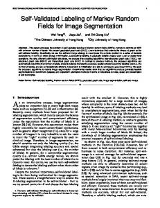
Figure 1. a) The robot and a portion of a 3D scan range map of Stanford University. b) Scan segmentation results obtained with SVM, Voted-SVM and AMN predictions. (Color legend: buildings/red, trees/green, shrubs/blue, ground/gray). the features of the objects xi ∈ IRdn and features of the relationships between them xij ∈ IRde . In 3D range data, the xi might be the spin image or spatial occupancy histograms of a point i, while the xij might include the distance between points i and j, the dot-product of their normals, etc. The simplest model of dependence of the potentials on the features is log-linear combination: log φi (k) = wnk · xi and log φij (k, k) = wek · xij , where wnk and wek are labelspecific row vectors of node and edge parameters, of size dn and de , respectively. Note that this formulation assumes that all of the nodes in the network share the same set of weights, and similarly all of the edges share the same weights. Stating the AMN restrictions in terms of the parameters w, we require that wek · xij ≥ 0. To ensure that wek · xij ≥ 0, we simply assume that xij ≥ 0, and constrain wek ≥ 0. The MAP problem for AMNs can be solved efficiently using a min-cut algorithm. In the case of binary labels (K = 2), the min-cut procedure is guaranteed to return the optimal MAP. For K > 2, the MAP problem is NPhard, but a procedure proposed by Boykov et al. [1], which augments the min-cut algorithm with an iterative procedure called alpha-expansion, guarantees a factor 2 approximation of the optimal solution. An alternative approach to solving the MAP inference problem is based on formulating the problem as an integer program, and then using a linear programming relaxation [2, 12]. This approach is slower in practice than the iterated min-cut approach, but has the same performance guarantees [21]. Importantly for our purposes, it forms the
as background. For simplicity of exposition, we focus our discussion to pairwise Markov networks, where nodes and edges are associated with potentials φi (Yi ) and φij (Yi , Yj ), ij ∈ E (i < j). In our task, edges are associated with links between points in the scan, corresponding to physical proximity; these edges serve to correlate the labels of nearby points. A node potential φi (Yi ) specifies a non-negative number for each value of the variable Yi . Similarly, an edge potential specifies non-negative number for each pair of values of Yi , Yj . Intuitively, a node potentials encodes a point’s “individual” preference for different labels, whereas the edge potentials encode the interactions between labels of related points. The joint distribution specified by the network is N Y 1 Y Pφ (y) = φi (yi ) φij (yi , yj ), Z i=1 ij∈E
where given by Z = P QNZ is the Qpartition 0function 0 0 φ (y ) φ (y , y ). The maximum ay0 i=1 i i ij∈E ij i j posteriori (MAP) inference problem in a Markov network is to find arg maxy Pφ (y). We further restrict our attention to an important subclass of networks, called associative Markov networks (AMNs) [21] that allow effective inference using graphcuts [8, 13]. These associative potentials generalize the Potts model [16], rewarding instantiations where adjacent nodes have the same label. Specifically, we require that φij (k, k) = λkij , where λkij ≥ 1, and φij (k, l) = 1, ∀k 6= l. We formulate the node and edge potentials in terms of 3
basis for our learning procedure. We represent an assignment y as a set of K ·N indicators {yik }, where yik = I(yi = k). With these definitions, the log of conditional probability log Pw (y | x) is given by: N X K K X XX (wnk · xi )yik + (wek · xij )yik yjk − log Zw (x). i=1 k=1
The standard approach of learning a conditional model w given (x, y ˆ) is to maximize the log Pw (ˆ y | x), with an additional regularization term, which is usually taken to be the squared-norm of the weights w [15]. An alternative method, recently proposed by Taskar et al. [22], is to maximize the margin of confidence in the true label assignment y ˆ over any other assignment y 6= y ˆ. They show that the margin-maximization criterion provides significant improvements in accuracy over a range of problems. It also allows high-dimensional feature spaces to be utilized by using the kernel trick, as in support vector machines. The maximum margin Markov network (M3 N) framework forms the basis for our work, so we begin by reviewing this approach. As in support vector machines, the goal in an M3 N is to maximize our confidence in the true labels y ˆ relative to any other possible joint labeling y. Specifically, we define the gain of the true labels y ˆ over another joint labeling y as:
ij∈E k=1
Note that the partition function Zw (x) above depends on the parameters w and input features x, but not on the labels yi ’s. Hence the MAP objective is quadratic in y. For compactness of notation, we define the node and edge weight vectors wn = (wn1 , . . . , wnK ) and we = (we1 , . . . , weK ), and let w = (wn , we ) be a vector of all the weights, of size d = K(dn + de ). Also, we define the node and edge labels vectors, yn = (. . . , yi1 , . . . , yiK , . . .)> and 1 K k ye = (. . . , yij , . . . , yij , . . .)> , where yij = yik yjk , and the vector of all labels y = (yn , ye ) of size L = K(N + |E|). Finally, we define an appropriate d × L matrix X such that log Pw (y | x) = wXy − log Zw (x).
log Pw (ˆ y | x) − log Pw (y | x) = wX(ˆ y − y). In M3 Ns, the desired gain depends on the number of misclassified labels in y, `(ˆ y, y), by scaling linearly with it:
The matrix X contains the node feature vectors xi and edge feature vectors xij repeated multiple times (for each label k), and padded with zeros appropriately. The linear programming formulation of the MAP problem for these networks can be written as: N X K K X XX k max (wnk · xi )yik + (wek · xij )yij (1) i=1 k=1
s.t.
yik
k yij ≤
X k yjk ,
yik = 1,
wX(ˆ y − y) ≥ γ`(ˆ y, y); ||w||2 ≤ 1.
Note that the number of incorrect node labels `(ˆ y, y) can also be written as N − y ˆn> yn . (Whenever yˆi and yi agree on some label k, we have that yˆik = 1 and yik = 1, adding 1 to y ˆn> yn .) By dividing through by γ and adding a slack variable for non-separable data, we obtain a quadratic program (QP) with exponentially many constraints: 1 min ||w||2 + Cξ (2) 2 s.t. wX(ˆ y − y) ≥ N − y ˆn> yn − ξ, ∀y ∈ Y.
ij∈E k=1
≥ 0, ∀i, k;
k yij ≤ yik ,
max γ s.t.
∀i;
∀ij ∈ E, k.
Note that we substitute the quadratic terms yik yik by varik k ables yij by using two linear constraints yij ≤ yik and k yij ≤ yik . This works because the coefficient wek · xij is non-negative and we are maximizing the objective function. k Hence yij = min(yik , yik ) at the optimum, which is equivk alent to yij = yik yjk if yik , yjk ∈ {0, 1}. In the binary case, the linear program Eq. (1) is guaranteed to produce an integer solution (optimal assignment) when a unique solution exists [21]. For K > 2, the LP may produce fractional solutions which are guaranteed to be within at most a factor of 2 of the optimal.
This QP has a constraint for every possible joint assignment y to the Markov network variables, resulting in an exponentially-sized QP. As our first step, we replace the exponential set of linear constraints in the max-margin QP of Eq. (2) with the single equivalent non-linear constraint: wXˆ y − N + ξ ≥ max wXy − y ˆn> yn . y∈Y
(3)
This non-linear constraint essentially requires that we find the assignment y to the network variables which has the highest probability relative to the parameterization wX − y ˆn> . Thus, optimizing the max-margin QP contains the MAP inference task as a component. The LP relaxation of Eq. (1) provides us with precisely the necessary building block to provide an effective solution for Eq. (3). The MAP problem is precisely the max subproblem in this QP. In the case of AMNs, this max subproblem can be replaced with the LP of Eq. (1). In effect, we are replacing the exponential constraint set — one which includes a constraint for every discrete y, with an infinite
4. Maximum margin estimation We now consider the problem of training the weights w of a Markov network given a labeled training instance (x, y ˆ). For simplicity of exposition, we assume that we have only a single training instance; the extension to the case of multiple instances is entirely straightforward. Note that, in our setting, a single training instance is not a single point, but an entire scene that contains tens of thousands of points. 4
5. Experimental results
constraint set — one which includes a constraintP for every k continuous vector y in Y 0 = {y : yik ≥ 0; k yi = k k k k 1; yij ≤ yi ; yij ≤ yi }, as defined in Eq. (1). After substituting the (dual of the) MAP LP into Eq. (3) and some algebraic manipulation (see [21]), we obtain: 1 min ||w||2 + Cξ (4) 2 N X s.t. wXˆ y−N +ξ ≥ αi ; we ≥ 0; i=1
X
αi −
We validated our scan segmentation algorithm by experimenting on two real-world and one synthetic datasets, which differed in both the type of 3D scanner used, and the types of objects present in the scene. We describe each set of experiments separately below. We compare the performance of our method to that of support vector machines (SVMs), a state-of-the-art classification method known to work well in high-dimensional spaces. The webpage
k αij
≥ wnk · xi − yˆik ,
∀i, k;
http://ai.stanford.edu/˜drago/Projects/Detector/
contains additional results, including a fly-through movie.
ij,ji∈E k k αij + αji ≥ wek · xij ,
k k αij , αji ≥ 0,
∀ij ∈ E, k.
Terrain classification. Terrain classification is useful for autonomous mobile robots in tasks such as path planning, target detection, and as a pre-processing step for other perceptual tasks. The Stanford Segbot Project (http://robots.stanford.edu/) has provided us with a laser range campus map collected by a robot equipped with a SICK2 laser scanner (see Fig. 1). The robot drove around a campus environment and acquired around 35 million scan readings. Each reading was a point in 3D space, represented by its coordinates in an absolute frame of reference, which was fairly noisy due to sensor noise and localization errors. Our task is to classify the laser range points into four classes: ground, building, tree, and shrubbery. Classifying ground points is trivial given their absolute z-coordinate; we do it by thresholding the z coordinate at a value close to 0. After this, we are left with approximately 20 million non-ground points. Each point is represented simply as a location in an absolute 3D coordinate system. The features we use require pre-processing to infer properties of the local neighborhood of a point, such as how planar the neighborhood is, or how much of the neighbors are close to the ground. We use features that are invariant to rotation in the x-y plane, as well as the density of the range scan, since scans tend to be sparser in regions farther from the robot. Our first type of feature is based on the principal plane around each point. To compute it, we sample 100 points in a cube of radius 0.5 meters. We run PCA on these points to get the plane, spanned by the first two principal components. We then partition the cube into 3 × 3 × 3 bins around the point, oriented with respect to the principal plane, and compute the percentage of points lying in the various subcubes. These percentages capture the local distribution well and are especially useful in finding planes. Our second type of feature is based on a column around each point. We take a cylinder of radius 0.25 meters, which extends vertically to include all the points in a “column”. We then compute what percentage of the points lie in various segments of this column (e.g., between 2m and 2.5m). Finally, we also use an indicator feature of whether a point lies within 2m of the ground. This feature is especially useful in classifying shrubbery.
Above, we also added the constraint we ≥ 0 to ensure positivity of the edge log-potentials. For K = 2, the MAP LP is exact, so that Eq. (4) learns exact max-margin weights for Markov networks of arbitrary topology. For K > 2, the linear relaxation leads to a strengthening of the constraints on w by potentially adding constraints corresponding to fractional assignments y. Thus, the optimal choice w, ξ for the original QP may no longer be feasible, leading to a different choice of weights. However, as our experiments show, these weights tend to do well in practice. The dual of Eq. (4) is given by: ¯¯ ¯¯2 N X K K N ¯¯ X 1 X ¯¯¯¯X k k k k ¯¯ max (1 − yˆi )µi − xi (C yˆi − µi )¯¯ ¯¯ ¯¯ ¯¯ 2 i=1 k=1 k=1 i=1 ¯¯ ¯¯2 ¯¯ K ¯¯ ¯¯ 1 X ¯¯¯¯ k X k k ¯¯ xij (C yˆij − µij )¯¯ − ¯¯λ + 2 ¯¯ ij∈E k=1 ¯¯ X µki = C, ∀i; s.t. µki ≥ 0, ∀i, k; µkij k
≥ 0,
µkij
≤
k k µi ,
µkij ≤ µkj ,
∀ij ∈ E, k;
λ ≥ 0, ∀k.
The primal and dual solution are related by: N X wnk = xi (C yˆik − µki ), i=1
wek
=
λk +
X
k xij (C yˆij − µkij ).
(5) (6)
ij∈E
One important consequence of these relationships is that the node parameters are all support vector expansions. Thus, the terms in the constraints of the form wn x can all be expanded in terms of dot products x> i xi ; similarly, the objective (||w||2 ) can be expanded similarly. Therefore, we can use kernels K(xi , xj ) to define node parameters. Unfortunately, the positivity constraint on the edge potentials, and the resulting λk dual variable in the expansion of the edge weight, prevent the edge parameters from being kernelized in a similar way. 5
a) Training instance
e)
c) SVM
b) AMN
f)
g)
d) AMN with edges ignored
h)
Figure 2. Segmentation results on the puppet dataset. a) Training set instance b) AMN segmentation result c) SVM segmentation result d) Result obtained by using the node weights learned by the AMN, and ignoring the MRF edges e) - h) Segmentation results on other testing set instances. (Color legend: head/green, torso/dark blue, limbs/red, background/gray). For training we select roughly 30 thousand points that represent the classes well: a segment of a wall, a tree, some bushes. We considered three different models: SVM, Voted-SVM and AMNs. All methods use the same set of features, augmented with a quadratic kernel. The first model is a multi-class SVM. This model (Fig. 1(b), right panel) achieves reasonable performance in many places, but fails to enforce local consistency of the classification predictions. For example arches on buildings and other less planar regions are consistently confused for trees, even though they are surrounded entirely by buildings. We improved upon the SVM by smoothing its predictions using voting. For each point we took its local neighborhood and assigned the point the label of the majority of its 100 neighbors. The Voted-SVM model (Fig. 1(b), middle panel) performs slightly better than SVM, yet it still fails in areas like arches of buildings where the SVM classifier has a locally consistent wrong prediction. The final model is a pairwise AMN. Each point is connected to 6 of its neighbors: 3 of them are sampled randomly from the local neighborhood in a sphere of radius 0.5m, and the other 3 are sampled at random from the vertical cylinder column of radius 0.25m. It is important to ensure vertical consistency since the SVM classifier is wrong in areas that are higher off the ground (due to the decrease in point density) or because objects tend to look different as we vary their z-coordinate (for example, tree trunks and tree crowns look different). While we experimented with a variety of edge features, we found that even using only a constant feature performs well.
We trained the AMN model using CPLEX to solve the quadratic program; the training took about an hour on a Pentium 3 desktop. For inference, we used min-cut combined with the alpha-expansion algorithm of Boykov et al. described above [1]. We split up the dataset into 16 square (in the xy-plane) regions, the largest of which contains around 3.5 million points. The implementation is largely dominated by I/O time, with the actual min-cut taking less than a minute even for the largest segment. We can see that the predictions of the AMN (Fig. 1 b), left panel) are much smoother: for example building arches and tree trunks are predicted correctly. We hand-labeled around 180 thousand points of the test set and computed accuracies of the predictions (excluding ground, which was classified by pre-processing). The differences are dramatic: SVM: 68%, Voted-SVM: 73% and AMN: 93%. Segmentation of articulated objects. We also tested our scan segmentation algorithm on a challenging dataset of cluttered scenes containing articulated wooden puppets. The dataset was acquired by a scanning system based on temporal stereo [4]. The system consists of two cameras and a projector, and outputs a triangulated surface only in the areas that are visible to all three devices simultaneously. The dataset contains eleven different single-view scans of three puppets of different sizes and in different positions. It also contains clutter and occluding objects such as rope, sticks and rings. Each scan has around 225, 000 points, which we subsampled to around 7, 000 with standard software. Our goal was to segment the scenes into 4 classes — puppet
6
AMN
SVM
a)
b)
c)
d)
Figure 3. Segmentation of vehicles (cars, trucks, suvs) from the background in synthetic range scans from the Princeton dataset. The AMN performs reasonably well on most of the testing scenes, as demonstrated in scenes a), b), and c). However, it sometimes fails to detect the vehicles in challenging scenes such as d). (Color legend: vehicles/green, background/pink). head, limbs, torso and background. Five of the scenes comprise our training set, and the rest are kept for testing. A sample scan from the training set is shown in Fig. 2a. To segment articulated objects, it is desirable to have an approach which is independent of global orientation altogether, and which discriminates based on shape alone. We used spin-images [11] as local point features. We computed spin-images of size 10 × 5 bins at two different resolutions. We scaled the spin-image values, and performed PCA to obtain 45 principal components, which comprised our point features. We use the surface links output by the scanner as edges in the MRF. Again, we experimented with several different edge features, but we got the best performance by using a constant feature for each edge. Because of clutter and occlusion in the scenes, our AMN framework achieves the best generalization performance when we keep the scope of the spin-images rather small (comparable to the size of the puppet’s head). Our scan segmentation algorithm performed very well by classifying 94.4% of the testing set points accurately, translating into 83.9% recall and 86.8% precision on the task of detecting puppet parts versus background. Overall, our results (see Fig. 2e–h) show that AMNs can detect puppet parts with a fairly high degree of accuracy, even under occlusion and clutter. The main source of classification error was the small puppet, which appears only in the testing set. By comparison, the SVM method applied to the same point features performs remarkably poorly (see Fig. 2c). The classification accuracy on the testing set is 87.16%, but that is because that the majority of points are classified as
background; indeed, overall the SVM approach achieves 93% precision but only 18.6% recall on the task of segmenting puppet parts against background. The poor performance is caused by the relatively small spin-image size which makes the algorithm more robust under clutter and occlusion, but at the same time makes it hard to discriminate between locally similar shapes. The dataset has significant shape ambiguity, as it is very easy to confuse sticks for limbs, and the torso for parts of the computer mouse appearing in the testing set. We tried to obtain a fairer comparison by changing the spin-image size to accommodate the SVM algorithm. The results were still significantly worse. To understand the reason underlying the superior performance of the AMN, we ran a flat classifier with node weights trained for the AMN model. The result, shown in Fig. 2d, suggests that our algorithm has an additional degree of flexibility — it can commit a lot of errors locally, but rely on the edge structure to eliminate the errors in the final result. This result demonstrates that our approach would be superior to a strategy which trains the edge and the node parameters separately. Princeton benchmark. The final test of our system was performed using a set of artificially generated scenes, which contain different types of vehicles, trees, houses, and the ground. Models of the objects in these scenes were obtained from the Princeton Shape Benchmark [20], and were combined in various ways to construct the training and test scenes. From these, a set of synthetic range scans were generated by placing a virtual sensor inside the scene. We cor-
7
References
rupted the ”sensor” readings with additive white noise. We then triangulated the resulting point cloud, and subsampled it down to our desired resolution. We trained both the SVM and the AMN approaches to distinguish vehicles from other objects and background. We used exactly the same node and edge features as in the puppet dataset, with the spin image size appropriately adjusted. The results, shown in Fig. 3, demonstrate again that our method outperforms the SVM method. In general, the AMN method labels most of the points on the vehicles correctly. Occasionally, the AMN method labels a flat part of a vehicle as background, because in this area, the features are indistinguishable from a wall, and the edge potentials are not strong enough to overcome this (see Fig. 3a). There are also cases in which the AMN method fails, as in Fig. 3d where we fail to detect the two cars under dense foliage. By comparison, the SVM method is only able to label vehicle parts with significant curvature, as flat areas are locally to similar to background. The AMN method thus provides a significant gain, producing a 93.76% overall accuracy, compared to only 82.23% for the SVM approach.
[1] Y. Boykov, O. Veksler, and R. Zabih. Fast approximate energy minimization via graph cuts. In ICCV, 1999. [2] Y. Boykov, O. Veksler, and R. Zabih. Markov random fields with efficient approximations. In CVPR, 1999. [3] C. Cortes and V. Vapnik. Support-vector networks. In Journal of Machine Learning, volume 20, 1995. [4] J. Davis, R. Ramamoorthi, and S. Rusinkiewicz. Spacetime stereo : A unifying framework for depth from triangulation. In CVPR, 2003. [5] A. Frome, D. Huber, R. Kolluri, T. Bulow, and J. Malik. Recognizing objects in range data using regional point descriptors. In Proc. ECCV, 2004. [6] T. Funkhouser, P. Min, M.Kazhdan, J. Chen, A. Halderman, D. Dobkin, and D. Jacobs. A search engine for 3d models. In ACM Trans. on Graphics, pages 22:83–105, January 2003. [7] G.Mori, S.Belongie, and J. Malik. Shape contexts enable efficient retrieval of similar shapes. In Proc. CVPR, 2001. [8] D. M. Greig, B. T. Porteous, and A. H. Seheult. Exact maximum a posteriori estimation for binar images. J. R. Statist. Soc. B, 51, 1989. [9] F. Han, Z. Tu, and S.-C. Zhu. Range image segmentation by an efficient jump-diffusion method. In IEEE Trans. on Pattern Analysis and Machine Intelligence, Sept 2004. [10] D. Huber, A. Kapuria, R. Donamukkala, and M. Hebert. Parts-based 3d object classification. In CVPR, 2004. [11] A. Johnson and M. Hebert. Using spin images for efficient object recognition in cluttered 3d scenes. In Proc. IEEE PAMI, volume 21, pages 433–449, 1999. [12] J. Kleinberg and E. Tardos. Approximation algorithms for classification problems with pairwise relationships: Metric labeling and Markov random fields. In FOCS, 1999. [13] V. Kolmogorov and R. Zabih. What energy functions can be minimized using graph cuts? In PAMI, 2002. [14] S. Kumar and M. Hebert. Discriminative fields for modeling spatial dependencies in natural images. In NIPS, 2003. [15] J. Lafferty, A. McCallum, and F. Pereira. Conditional random fields: Probabilistic models for segmenting and labeling sequence data. In ICML, 2001. [16] R. B. Potts. Some generalized order-disorder transformations. Proc. Cambridge Phil. Soc., 48, 1952. [17] R.Osada, T.Funkhouser, B. Chayelle, and D. Dobkin. Matching 3d models with shape distributions. In Shape Modeling International, May 2001. [18] S. Ruiz-Correa, L. Shapiro, and M. Meila. A new paradigm for recognizing 3-d object shapes from range data. In CVPR, 2003. [19] S. Ruiz-Correa, L. Shapiro, M. Meila, and G.Berson. Discriminating deformable shape classes. In NIPS, 2004. [20] P. Shilane, P. Min, M. Kazhdan, and T. Funkhouser. The princeton shape benchmark. Shape Modeling International, 2004. [21] B. Taskar, V. Chatalbashev, and D. Koller. Learning associative Markov networks. In Proc. ICML, 2004. [22] B. Taskar, C. Guestrin, and D. Koller. Max margin Markov networks. In NIPS, 2003. [23] A. Torralba, K. Murphy, and W. Freeman. Contextual models for object detection using boosted random fields. In NIPS, 2004.
6. Conclusions We present an MRF-based method for detection and segmentation of complex objects and object classes from 3D range data. Our approach has a number of attractive theoretical and practical properties. By constraining the class of MRFs to be solvable by graph-cuts, our models are efficiently learned using a compact quadratic program, and at run-time, scale up to tens of millions of points and multiple object classes. The proposed learning formulation effectively and directly learns to exploit a large set of complex surface and volumetric features, while balancing the spatial coherence modeled by the MRF. There are several interesting directions in which our work can be extended, that address the main limitation of our work: its reliance on local features to distinguish objects. First, as our formulation is based on the max-margin framework underlying SVMs, we can easily incorporate kernels in order to further boost the expressive power of the models. We are currently developing appropriate spatial kernels. More importantly, our method relies heavily on the existence of distinguishing local surface features of objects. Since we do not model object parts and spatial relations between them, our method is effective at differentiating between mostly homogeneous objects (for example, trees, buildings, limbs), which do not have many parts that “look” similar locally. For example, it would be difficult to differentiate between car types, such as sedan vs. coup, which look alike except for the rear door/trunk. The challenge of incorporating the object/part hierarchy into the learning framework is a subject of our future work. 8