Self-Validated Labeling of Markov Random Fields for ... - CiteSeerX

IEEE TRANSACTIONS ON PATTERN ANALYSIS AND MACHINE INTELLIGENCE, ACCEPTED FOR PUBLICATION

1

Self-Validated Labeling of Markov Random Fields for Image Segmentation Wei Feng†‡ , † The

Jiaya Jia† ,

Chinese University of Hong Kong

and Zhi-Qiang Liu‡ ‡ City

University of Hong Kong

Abstract—This paper addresses the problem of self-validated labeling of Markov random fields (MRFs), namely to optimize an MRF with unknown number of labels. We present graduated graph cuts (GGC), a new technique that extends the binary s-t graph cut for self-validated labeling. Specifically, we use the split-and-merge strategy to decompose the complex problem to a series of tractable subproblems. In terms of Gibbs energy minimization, a suboptimal labeling is gradually obtained based upon a set of cluster-level operations. By using different optimization structures, we propose three practical algorithms: tree-structured graph cuts (TSGC), netstructured graph cuts (NSGC) and hierarchical graph cuts (HGC). In contrast to previous methods, the proposed algorithms can automatically determine the number of labels, properly balance the labeling accuracy, spatial coherence and the labeling cost (i.e., the number of labels), and are computationally efficient, independent to initialization and able to converge to good local minima. We apply the proposed algorithms to natural image segmentation. Experimental results show that our algorithms produce generally feasible segmentations for benchmark datasets, and outperform alternative methods in terms of robustness to noise, speed and preservation of soft boundaries. Index Terms—Self-validated labeling, Markov random fields (MRFs), graduated graph cuts, image segmentation, split-and-merge.

F

1

I NTRODUCTION

A

S an intermediate process, image segmentation plays an important role in many high-level vision tasks, such as recognition [1]–[3] and authentication [4]. Recently, many methods have been proposed for 𝐾labeling segmentation, which mainly concern the balance of segmentation quality and computational efficiency, under the assumption that the number of labels 𝐾 is known [5]–[10]. However, this assumption makes them highly unsuitable for recent content-based applications, such as generic object recognition [11], since for a large number of images it is very infeasible to ask the users to input the “right” number of segments for each individual image. Therefore, in image segmentation, we should consider not only the labeling quality (i.e., the Gibbs energy integrating labeling accuracy and spatial coherence) but also the labeling cost (i.e., the number of labels). In general, for a comparable segmentation quality (i.e., similar Gibbs energy value), we should prefer the labeling with the least number of labels due to Occam’s razor. For clarity, we use the term self-validated labeling to denote the labeling problem when the number of labels is unknown.1 Despite the practical importance, self-validated labeling is far from being well-studied for image segmentation. There seems a straightforward way to extend the 𝐾-labeling segmentation to be self-validated - that is, we try several particular 𝐾 and choose the best labeling 1. The term self-validated labeling (or self-validation) is borrowed from clustering validation [12], where the number of clusters is a very important aspect to be validated.

result with the smallest 𝐾. However, this is highly impractical, especially for a large number of images, where complexity is the most obstacle (see Sec. 4.4 for details). In addition, some 𝐾-labeling methods may lead to unsatisfactory segmentations, even when fed by the “correct” number of labels. See Fig. 1(b) for example. For the synthesized image in Fig. 1(a), normalized cut [6], a state-of-the-art 𝐾-labeling method, is unable to generate satisfying segmentation using the correct number of labels 5. It can produce all “right” boundaries, together with many false-alarmed boundaries, only by feeding with a much larger number of labels 20. Indeed, the drawback of 𝐾-labeling segmentation emphasizes the practical necessity of self-validated labeling. As shown in Fig. 1(c), there exist some self-validated methods in the literature [13]–[16]. However, few of them succeed in both computational efficiency and robustness to noise distortion. For instance, split-andmerge is a natural strategy for self-validated segmentation (see GBS in Fig. 1(c) for example) and has a long history [17]. In general, existing split-and-merge methods are able to efficiently determine all salient regions of an image by coarse-to-fine partitioning (e.g., IsoCut [18]) and/or fine-to-coarse aggregation (e.g., SWA [19]). By using advanced optimization techniques, such as spectral relaxation in SWA, recent split-and-merge methods have largely improved their accuracy and flexibility. More importantly, most of them are self-validated and efficient. However, these methods are usually not robust enough to noise distortion. In contrast, 𝐾-labeling methods are accurate, robust but not self-validated. Therefore, a reliable labeling method, which can auto-


2

(a) Original (#seg=5)

(#seg=8)

(#seg=10)

(#seg=15)

(#seg=20)

(b) K -labeling segmentation (normalized cut)

GBS (#seg=19)

MeanShift (#seg=328) TS-MRF (#seg=49)

DDMCMC (#seg=5)

(c) Self-validated segmentation (previous methods)

TSGC (#seg=5)

NSGC (#seg=5)

HGC (#seg=6)

(d) Self-validated segmentation (our methods)

Fig. 1. Comparison of self-validated and 𝐾-labeling segmentation for the synthesized image (a) (of size 128 × 128, consisting of 5 segments and with 40% Gaussian noise). We show the segmentation results of normalized cut (NCut) [6], which is a representative 𝐾-labeling method, and four state-of-the-art self-validated methods (efficient graph-based segmentation (GBS) [13], MeanShift [14], tree-structured MRF (TS-MRF) [15] and data-driven Markov Chain Monte Carlo (DDMCMC) [16]) in (b) and (c), respectively. The average running time of NCut for image (a) is 11.4s. However, NCut is unable to return satisfying result when fed by the correct number of segments 5; it can produce all “right” boundaries, mixed with many “wrong” boundaries, only when fed by a much larger number of segments 20. Bottom-up methods, such as MeanShift and GBS, can automatically determine the number of segments and are very fast (need about 1s), but are either apt to oversegmentation or too sensitive to noise corruption. TSMRF uses split-and-merge strategy in the MRF framework, but the approximate optimization cannot guarantee spatially coherent labeling. DDMCMC generates reasonable result with right number of segments, but it is very slow and needs about 210s to reach a stable labeling for image (a). The results of the proposed algorithms are shown in (d). Note that, TSGC needs 2.96s, NSGC needs 5.70s, HGC needs 2.01s, and all of them produce satisfying results with reasonable number of segments. matically determine the number of labels and optimize a global objective function, is of significant importance both theoretically and practically. In this paper, we address this problem and study how to “suboptimally” label an MRF with unknown number of labels. Our work aims at seeking a simple yet principled way to decompose the intractable self-validated labeling problem to a series of tractable subproblems. We start from the graph theoretic formulation of image segmentation. It is Greig et al. that first showed the binary labeling problem can be exactly solved by s-t graph mincut/maxflow (s-t graph cut for short) [20]. Recently, Boykov et al. horizontally extended the binary s-t graph cut to solve the 𝐾-labeling problem [21]– [23], which was further theoretically investigated by Kolmogorov et al. [24], [25]. Except for being not selfvalidated, the horizontal extension, as shown by our experiments, is highly dependent on the initialization. We propose an alternative way to vertically extend the

binary s-t graph cut to solve the self-validated labeling problem.2 The core of our approach is to gradually reconstruct a suboptimal segmentation based on a set of cluster-level operations: retaining, splitting, merging and regrouping. These operations lead to a suboptimal topdown labeling refinement process, which intrinsically solves the self-validation problem of MRFs labeling. Because we gradually refine the labeling using s-t graph cut, we name our approach graduated graph cuts (GGC). Using different optimization structures, we propose three concrete algorithms: tree-structured graph cuts 2. The term vertical/horizontal extension is derived from the algorithmic structure of segmentation methods, which refers to whether a segmentation algorithm explores the space of all possible labelings directly or in a hierarchical manner. As shown in Fig. 6, the proposed GGC scheme uses the s-t graph cut to gradually refine the labeling between two consecutive levels in the hierarchical structure, thus can be viewed as a vertical extension to binary s-t graph cut. In contrast, 𝛼expansion and 𝛼-𝛽-swap use the s-t graph cut to iteratively refine the 𝐾-labeling at the same level, thus belonging to horizontal extension.

W. FENG et al.: SELF-VALIDATED LABELING OF MARKOV RANDOM FIELDS FOR IMAGE SEGMENTATION

(TSGC), net-structured graph cuts (NSGC) and hierarchical graph cuts (HGC), within the GGC scheme. All of them start by treating the whole image as a single segment, then iteratively select the optimal operation for each segment, and end when the overall energy stops decreasing. Based on extensive experiments and a qualitative analysis, we show that by this process the proposed algorithms always obtain good local minima.

2

R ELATED W ORK

Image segmentation remains a classical and active topic in low-level vision for decades. Among the previous successful methods, MRF-based ones account for a large percentage [26]. In recent years, it is still a dynamic area that studies the application of MRFs in image segmentation, such as double MRF [27], data-driven MCMC [16], hidden Markov measure field model [28] and treestructured MRF [15]. MRF-based methods can naturally represent the labeling accuracy and spatial coherence within the Bayesian framework, but some of them are computationally complex and converge slowly. Recently, graph theoretic approaches have been successfully used in MRFs labeling [5]–[9], [18], [29]. These methods treat image segmentation as a graph partitioning problem. By using advanced optimization techniques, they realize efficient energy minimization and properly balance the labeling quality and computational efficiency. According to the particular energy function they minimize, graph theoretic approaches fall into two categories: continuous methods and discrete methods. Representative continuous segmentation methods include spectral relaxation [6], [30]–[33] and random walk [7]–[9]. By encoding local pairwise similarity into a graph, continuous methods usually minimize a relaxed partitioning function by solving a constrained eigenproblem [6] or a linear system [9]. Since continuous methods generate fractional labeling, they were successfully used in image matting [34], [35]. In contrast, typical discrete methods, such as s-t graph cut [20] and its extensions [21]–[25], directly solve the original integer-programming for graph partitioning. One desirable property of discrete methods is that, for a particular set of binary energy functions (e.g., submodular functions [24], [25]), they can obtain a globally optimal labeling in polynomial time. Since in image segmentation the widely-used pairwise terms based on Potts model are usually submodular, discrete segmentation methods usually have better theoretical guarantee, especially in binary case. For instance, binary s-t graph cut has achieved great success in interactive foreground segmentation [36]–[38]. Although discrete methods guarantee a global minimum for some particular energy forms, they cannot handle generic energy functions [39], while continuous methods have no such limit. Moreover, continuous MRF models have recently been shown their potential in rectifying the shrinkage bias of discrete models in seeded image segmentation [7], [8]. Despite

3

the respective merits of discrete and continuous methods in image segmentation, how to properly take account of the labeling cost (i.e., the number of labels) within the optimization framework (for either discrete or continuous models) still remains an open problem. Before image segmentation, graph partitioning has been widely used in parallel simulation and the design of VLSI. There are some well-established graph partitioning packages, such as METIS [40], which use multilevel split-and-merge to seek a balanced minimal partition to the graph using the Kernighan-Lin algorithm. Despite their successes in other areas, they are not readily suitable for image segmentation, since they cannot maintain spatial coherence well, are not guaranteed to be optimal and biased for image segmentation. For instance, the normalized cut criterion was proposed to rectify the small partition bias of minimum cut criterion for image segmentation [6]. The improvement can be clearly seen in Fig. 16. But, the split-and-merge strategy does shed light on self-validated labeling, since many splitand-merge segmentation methods are self-validated [13], [18]. Note that there is a long history of split-and-merge in image segmentation [17]. Recent methods, such as IsoCut [18] and GBS [13], integrate advanced optimization techniques into the split-and-merge scheme, thus significantly improving the performance. However, as shown by our experiments (see Fig. 12 and 13), they are usually sensitive to noise distortion. In this paper, we try to find a principled way to apply the split-and-merge strategy to a global optimization framework, thus integrating the merits of both schemes and realizing reliable self-validated labeling. In contrast to Boykov’s horizontal extension to binary s-t graph cut by iteratively refining the labeling between the 𝐾 segments [21], our GGC approach can be viewed as a vertical extension. We show how to gradually use the binary s-t graph cut to efficiently minimize the Gibbs energy downward, thus solving the self-validated labeling problem. Our work is also partially related to clustering, e.g., AutoClass [41] uses a mixture prior model and the Bayesian method to determine the optimal classes, which intrinsically favors clustering with less numbers of clusters. Another related work is TS-MRF [15] that reduces the 𝐾-labeling segmentation into a sequence of 𝐾 − 1 simpler binary segmentations. However, the suboptimality property of TS-MRF is unclear, and as shown in our experiments, the approximate labeling of TS-MRF may arbitrarily deviate from good local minima, thus severely degrading the performance. Partial work and some preliminary results of this paper were also reported in [29].

3

G RAPH F ORMULATION FOR S EGMENTATION

The Bayesian framework and MRFs model form a solid foundation for image segmentation, based on which an image 𝐼 is modeled as an MRF 𝑋 with observation 𝑌 . The MRF 𝑋 = {𝑥𝑝 } represents the segmentation result


4

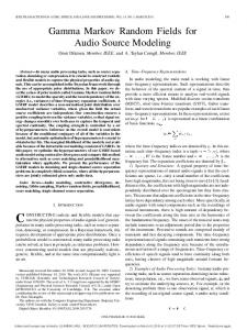
likelihood arc E L

label vertex VL

coherence arc E C

pixel vertex VP

we show that our approach is good at preserving soft boundaries using the simple 4-connected lattice only, which results in high computational efficiency. In terms of MRFs, the statistically optimal labeling ˆ maximizes the posteriori probability (MAP) given 𝑋 ˆ = arg max𝑋 𝑃 (𝑋∣𝑌 ), which is observation 𝑌 , i.e., 𝑋 equivalent to minimizing the following Gibbs energy: ∑ ∑ 𝐸(𝑋 ∣ 𝑌 ) = 𝐸lik (𝑥𝑝 ∣ 𝑦𝑝 ) + 𝐸coh (𝑥𝑝 , 𝑥𝑞 ), (1) (𝑥𝑝 , 𝑣𝑝 )∈ℰL

(a)

L1

L2

Lk

VL VP VL

EL

VP E L E C (b)

(c)

Fig. 2. Graph formulation of MRF-based segmentation (by 4-connected lattice): (a) undirected graph 𝒢 = ⟨𝒱, ℰ⟩ with 𝐾 segments {𝐿1 , . . . 𝐿𝐾 } and the observation 𝑌 ; (b) final segmentation corresponds to a multiway cut of the graph 𝒢; (c) the relationship of vertices and edges in the graph formulation.

that considers both accuracy and contextual constraints, where 𝑥𝑝 ∈ ℒ, 𝑝 is an image pixel and ℒ = {𝐿1 , 𝐿2 , . . .} is the label space. The goal of self-validated segmentation is to estimate the optimal label for each pixel when the number of labels 𝐾 = ∣ℒ∣ is unknown. As shown in Fig. 2(a), we can equivalently interpret the MRF model with a graph formulation, where the image 𝐼 and the contextual dependency is represented by an undirected graph 𝒢 = ⟨𝒱, ℰ⟩. In particular, the vertex set 𝒱 = {𝒱L , 𝒱P } is composed of two components: the set of label vertices 𝒱L and the set of pixel vertices 𝒱P . From Fig. 2, we can see that each 𝑣𝑝 (𝑣𝑝 ∈ 𝒱P ) corresponds to a pixel 𝑝, with 𝑦𝑝 denoting its observation and 𝑥𝑝 (𝑥𝑝 ∈ 𝒱L ) denoting its potential label. The arc set ℰ = {ℰL , ℰC } also consists of two parts: the likelihood arcs ℰL = {(𝑣𝑙 , 𝑣𝑝 )∣𝑣𝑙 ∈ 𝒱L and 𝑣𝑝 ∈ 𝒱P } representing the likelihood of labeling pixel 𝑝 with 𝑣𝑙 (𝑣𝑙 = 𝐿𝑙 ), and the coherence arcs ℰC = {(𝑣𝑝 , 𝑣𝑞 )∣(𝑣𝑝 , 𝑣𝑞 ) ∈ 𝒱P2 and (𝑝, 𝑞) ∈ 𝒩2 } reflecting the pairwise dependency between adjacent pixels. Here 𝒩2 denotes the second order neighborhood system. Although the proposed approach can handle dense graphs with long-range pairwise connections of any type, we focus on the 4-connected lattice in this paper. Note that, in MRFs labeling, it has been shown that properly encoding long-range connections helps to improve the labeling specificity [42]–[44]. In image segmentation, this means that dense graphs with longrange connections may benefit the preservation of soft boundaries. However, the cost is a significant increase to the complexity of graph partitioning. In contrast,

(𝑣𝑝 , 𝑣𝑞 )∈ℰC

where 𝐸lik (𝑥𝑝 ) is the likelihood energy represents the goodness of labeling pixel 𝑝 by 𝑥𝑝 , and 𝐸coh (𝑥𝑝 , 𝑥𝑞 ) is the coherence energy denoting the prior of labeling spatial coherence. For simplicity, in the rest of the paper, we use 𝐸(𝑋) to represent the Gibbs energy 𝐸(𝑋∣𝑌 ), use 𝐸lik (𝑒𝑝 ) (𝑒𝑝 = {𝑥𝑝 , 𝑣𝑝 } ∈ ℰL ) to represent 𝐸lik (𝑥𝑝 ∣𝑦𝑝 ), and use 𝐸coh (𝑒𝑝𝑞 ) (𝑒𝑝𝑞 = {𝑣𝑝 , 𝑣𝑞 } ∈ ℰC ) to represent 𝐸coh (𝑥𝑝 , 𝑥𝑞 ). Then, we can rewrite Eq. (1) as ∑ ∑ 𝐸(𝑋) = 𝐸lik (𝑒𝑝 ) + 𝐸coh (𝑒𝑝𝑞 ). (2) 𝑒𝑝 ∈ℰL

𝑒𝑝𝑞 ∈ℰC

Referring to Fig. 2(a), if we assign 𝐸lik (𝑒𝑝 ) as the weight of likelihood arc 𝑒𝑝 and 𝐸coh (𝑒𝑝𝑞 ) as the weight of coherence arc 𝑒𝑝𝑞 , the optimal segmentation with minimal Gibbs energy corresponds to the minimal multiway cut of weighted graph 𝒢 (see Fig. 2(b)). Let Seg(𝐼) = {𝑆𝑖 }𝐾 𝑖=1 represent the final segmentation of image 𝐼 consisting of 𝐾 nonoverlapping segments 𝑆1 , . . . , 𝑆𝐾 , each of which has a unique label 𝐿(𝑆𝑖 ) ∈ ℒ and 𝐿(𝑆𝑖 ) ∕= 𝐿(𝑆𝑗 ) when 𝑖 ∕= 𝑗. A particular segment 𝑆 corresponds to a set of pixels having the same label, i.e., 𝑆 = {𝑣∣𝑣 ∈ 𝒱P and 𝐿(𝑣) = 𝐿(𝑆)}, where 𝐿(𝑣) and 𝐿(𝑆) denote the labels of pixel 𝑣 and segment 𝑆 respectively. We use 𝐹 (𝑆) to represent the corresponding feature space of 𝑆, i.e., 𝐹 (𝑆) = {𝑦𝑝 ∣𝑣𝑝 ∈ 𝑆}. From Eqs. (1) and (2), we can express the likelihood and coherence energy functions of segment 𝑆 as ∑ 𝐸lik (𝑆) = 𝐸lik (𝐿(𝑆) ∣ 𝑦𝑝 ), (3) (𝐿(𝑆), 𝑣𝑝 )∈ℰL 𝑣𝑝 ∈𝑆

∑

𝐸coh (𝑆) =

𝐸coh (𝑥𝑝 , 𝑥𝑞 ).

(4)

(𝑣𝑝 , 𝑣𝑞 )∈ℰC 𝑣𝑝 ∈𝑆 ∧ 𝑣𝑞 ∈𝑆 /

Specifically, the coherence energy of segment pair (𝑆𝑖 , 𝑆𝑗 ) (𝑆𝑖 ∕= 𝑆𝑗 ) is ∑ 𝐸coh (𝑆𝑖 , 𝑆𝑗 ) = 𝐸coh (𝑥𝑝 , 𝑥𝑞 ). (5) (𝑣𝑝 , 𝑣𝑞 )∈ℰC 𝑣𝑝 ∈𝑆𝑖 ∧ 𝑣𝑞 ∈𝑆𝑗

∑ It is clear that 𝐸coh (𝑆𝑖 ) = 𝑗∕=𝑖 𝐸coh (𝑆𝑖 , 𝑆𝑗 ). Based on Eqs. (1)–(5), we can express the Gibbs energy of segmentation Seg(𝐼) as ( ) 𝐸 Seg(𝐼)

=

𝐾 ∑

𝐸lik (𝑆𝑘 ) +

𝑘=1

=

𝐾 ( ∑ 𝑘=1

𝐾 ∑

𝐸coh (𝑆𝑖 , 𝑆𝑗 )

𝑖,𝑗=1

𝐸coh (𝑆𝑘 ) ) . 𝐸lik (𝑆𝑘 ) + 2

(6)


Graph formulation reveals the equivalence between MRF-based segmentation and the NP-complete multiway (𝐾-way) graph cut problem [21], [45]. Furthermore, when the number of labels 𝐾 is unknown, the problem becomes even more difficult. Nevertheless, for 𝐾 = 2, it is equivalent to the classical graph mincut/maxflow problem, which can be exactly minimized in polynomial time [21]–[24], [46]. 3.1 Optimal Binary Segmentation Let us first see how to use the s-t graph cut to achieve an optimal binary segmentation, i.e., labeling all pixels with a binary MRF 𝑋 b = {𝑥𝑝 } (𝑥𝑝 ∈ {0, 1}) based on observation 𝑌 . When 𝐾 = 2, the Gibbs energy of segmentation becomes ∑ ∑ b b 𝐸 b (𝑋) = 𝐸lik (𝑒𝑝 ) + 𝐸coh (𝑒𝑝𝑞 ). (7) 𝑒𝑝 ∈ℰL

5

Input: Feature space 𝑌 . Output: Two-level component/subcomponent feature 1 𝐻 model {𝐶 0 , 𝐶 1 } = {{𝑀ℎ0 }𝐻 ℎ=1 , {𝑀ℎ }ℎ=1 }. 1. Dividing feature samples into two components 𝐶 0 and 𝐶 1 by 𝐾-means; 2. Subdividing 𝐶 0 and 𝐶 1 into 𝐻 subcomponents 𝑀ℎ0 and 𝑀ℎ1 by 𝐾-means respectively; 3. Deriving the representative center for each subcomponent and obtaining the final model 1 𝐻 𝑌 = {𝐶 0 , 𝐶 1 } = {{𝑀ℎ0 }𝐻 ℎ=1 , {𝑀ℎ }ℎ=1 };

Algorithm 1: Two-level nonparametric feature model.

use a fast K-means algorithm in our scheme with triangle inequality acceleration [47]. Besides, the nonparametric representation helps to improve the ability of our model to handle non-Gaussian color distributions in an image.

𝑒𝑝𝑞 ∈ℰC

As we have known, a particular difficulty in segmentation is that one has to estimate both the representative model of each segment and its corresponding regions at the same time [28]. Thus, we need an effective feature model to represent each segment, and based on which b b to define the concrete energy function of 𝐸lik and 𝐸coh .

3.1.2 Energy Assignment The likelihood energy measures the segmentation accuracy and can be viewed as the intra-segment distance. Based on the nonparametric representation of feature space, we define the likelihood energy as ( )𝛼 b 𝐸lik (𝑥𝑝 ) = 𝑑1𝑝 𝑥𝑝 + 𝑑0𝑝 (1 − 𝑥𝑝 ) , (8) where 𝑑0𝑝 = 𝐷(𝑦𝑝 , 𝐶 0 ) and 𝑑1𝑝 = 𝐷(𝑦𝑝 , 𝐶 1 ) that represent the distance between 𝑦𝑝 and 𝐶 0 and 𝐶 1 respectively, and 𝐷(𝑦𝑝 , 𝐶 𝑡 ) = min ∥𝑦𝑝 − 𝑀ℎ𝑡 ∥, 𝑡 ∈ {0, 1}. ℎ

(a)

(b)

Fig. 3. Nonparametric feature model for a segment with obser-

vation 𝑌 (𝐻 = 3): (a) is the two-level component/subcomponent representation, (b) shows an example.

3.1.1 Feature Space Representation To achieve an effective energy assignment and efficient computation, we use Algorithm 1 to derive a two-level (component/subcomponent) nonparametric feature model for a segment with observation feature space 𝑌 (see Fig. 3 for illustration). Specifically, for a given segment 𝑆, its feature space is characterized by 2 components (used to compute the optimal segment splitting energy) and 2𝐻 subcomponents (used to compute the segment retaining and merging energy). Details about their functions can be found in Eqs.(8)–(11) and Sec. 4. Note that our feature model is nonparametric that is in contrast to the GMM modeling in GrabCut [38]. We choose the nonparametric manner mainly due to the consideration of efficiency. As we know, the EM estimation of GMM model needs an iterative process. It is unsuitable for self-validated segmentation, since we may need to model a large number of segments as opposed to the two segments in GrabCut. Instead, we

(9)

From Eq. (9), we can also define the distance between two components as ) ( (10) Dist(𝐶 0 , 𝐶 1 ) = min min 𝐷(𝑀𝑖𝑡 , 𝐶 1−𝑡 ) . 𝑡∈{0,1}

𝑖

Note that in Eq. (8), 𝛼 controls the influence of likelihood b energy 𝐸lik on the Gibbs energy 𝐸 b . The larger the 𝛼 is, b the more important is the likelihood energy 𝐸lik in 𝐸 b . The coherence energy measures the segmentation feasibility that represents the contextual prior. We define the coherence energy by extending the classical Potts model [22], [29]: b 𝐸coh (𝑥𝑝 , 𝑥𝑞 ) =

( ∥𝑦𝑝 − 𝑦𝑞 ∥ ) ∣𝑥𝑝 − 𝑥𝑞 ∣ exp − . ∥𝑝 − 𝑞∥ 𝛽

(11)

b Our definition of 𝐸coh encourages close pixels with similar colors to have the same label. In Eq. (11), 𝛽 b controls the influence of the coherence energy 𝐸coh on b the Gibbs energy 𝐸 . The larger the 𝛽 is, the more b role of the coherence energy 𝐸coh plays in 𝐸 b .3 Fig. 4 compares the extended Potts model and the classical Potts model for image segmentation. We can clearly see that the extended model makes the coherence prior more flexible, since with comparable number of segments

3. It has been shown that the Ising and Potts models cannot provide sufficient smoothing guidance if used as an image-specific prior [48]. As a general (i.e., image-independent) smoothing prior, the Potts model has been widely-used in MRFs labeling [21]–[24], [29], [36]–[38].


6

Extended Potts Model (#seg=22)

Refinement by cluster-level operations

Webtext Image (50% Gaussian noise)

Retaining

Merging

Splitting

Regrouping

Final Result (#seg=21)

Start from one segment

Fig. 5. Working flow of the proposed GGC scheme.

Classical Potts Model (#seg=24) Classical Potts Model (#seg=55)

Fig. 4. Comparison of the extended and classical Potts model for image segmentation.

the extended data-driven Potts model generates more accurate labeling, while the classical Potts model needs more than twice number of segments to achieve the similar accuracy level.

4

G RADUATED G RAPH C UTS

In this section, we will show how to vertically extend the binary s-t graph cut to solve the self-validated labeling problem for image segmentation. The core of our approach is to gradually refine the labeling according to the Gibbs energy minimization principle. Our segmentation refinement is based on the following four types of segment-level operations. (1) Retaining (=): For segment 𝑆, keeping 𝑆 unchanged, as denoted by 𝑆 = 𝑆. (2) Splitting (→): For segment 𝑆, splitting 𝑆 into two isolated parts 𝑆˜0 and 𝑆˜1 with minimal binary Gibbs energy Eq. (7) using s-t graph cut, as denoted by 𝑆 → (𝑆˜0 , 𝑆˜1 ). (3) Merging (∪): For segment 𝑆, merging 𝑆 with its nearest neighbor Near(𝑆) to form a new segment 𝑆 ′ , expressed as 𝑆 ∪ Near(𝑆) = 𝑆 ′ . Near(𝑆) is defined by Definition 3. (4) Regrouping: For each segment pair (𝑆𝑖 , 𝑆𝑗 ), merging them together and then re-splitting the merged segment to 𝑆𝑖′ and 𝑆𝑗′ using binary s-t graph cut to refine the labeling. This process is denoted as 𝑆𝑖 ∪ 𝑆𝑗 → (𝑆𝑖′ , 𝑆𝑗′ ). Segment regrouping is particularly useful in the HGC algorithm to refine the

labeling inherited from the coarse scale. Detailed introduction can be found in Sec. 4.3. Fig. 5 shows the working flow of the proposed GGC scheme. In general, it is a top-down refinement process. The image is treated as one segment at first. Each segment 𝑆 is modeled by a binary MRF 𝑋 b , based on which we iteratively refine the labeling by adjusting each segment with the optimal operation according to the energy minimization principle. This refinement process is terminated when all segments remain unchanged. Since optimizing a binary MRF with s-t graph cut is much easier than solving a flat 𝐾-label MRF, the GGC labeling is much faster than classical MRF methods [26]. Using different operations and optimization structures, we propose three segmentation algorithms: tree-structured graph cuts (TSGC), net-structured graph cuts (NSGC) and hierarchical graph cuts (HGC). We will elaborate each algorithm in the following. 4.1

Tree-Structured Graph Cuts (TSGC)

We first analyze the situation of allowing only two types of operations, i.e., segment retaining and splitting. Accordingly, the GGC scheme shown in Fig. 5 is concretized to a tree-structured evolution process, as shown in Fig. 6(a). At the beginning, the image 𝐼 is treated as one segment, i.e., Seg(0) (𝐼) = {𝑆0 }. The initial segment 𝑆0 can be modeled as a binary MRF 𝑋0b . Using the nonparametric representation of 𝐹 (𝑆0 ) and corresponding energy assignment Eqs. (7)–(11), we can obtain an optimal splitting of 𝑆0 → (𝑆˜00 , 𝑆˜01 ) in terms of Gibbs energy minimization, where 𝑆˜00 and 𝑆˜01 are two tentative segments derived from 𝑆0 using binary s-t graph cut. If the splitting is better than retaining 𝑆0 unchanged, we update 𝑆0 to 𝑆˜00 and 𝑆˜01 . Accordingly, the segmentation is updated to Seg(1) (𝐼) = {𝑆1 , 𝑆2 } with 𝑆1 = 𝑆˜00 and 𝑆2 = 𝑆˜01 . We then model each segment 𝑆𝑖 separately with binary MRF 𝑋𝑖b and find the optimal operation according to the principle of energy minimization. We continue this process iteratively until for all segments operation retaining is better than splitting. We can see that this is an iterative segment evolution process, which is terminated when all tentative segments remain unchanged, then we obtain the final segmentation Seg(𝐼). In the following, we give formalized description of TSGC algorithm. Definition 1: Given two operations 𝐴 and 𝐵, we say 𝐴 is better than 𝐵 for segment 𝑆 iff one of the following

W. FENG et al.: SELF-VALIDATED LABELING OF MARKOV RANDOM FIELDS FOR IMAGE SEGMENTATION 0

3

Referring to Eqs. (3) and (5) for concrete definitions of 𝐸lik (𝑆) and 𝐸coh (𝑆𝑖 , 𝑆𝑗 ), respectively. Specifically, for segment 𝑆, the likelihood energy 𝐸lik (𝑆), referring to Eq. (8), can be viewed as the overall distance between all feature samples to the subcompo∑ nents, i.e., 𝐸lik (𝑆) = 𝑦𝑝 ∈𝐹 (𝑆) 𝐷(𝑦𝑝 , 𝐶 𝑥𝑝 ). If treating 𝑆 as one segment, we use 2𝐻 subcomponents to represent 𝐹 (𝑆). By splitting 𝑆 into two segments 𝑆˜0 and 𝑆˜1 , we use 4𝐻 subcomponents to represent 𝐹 (𝑆). Since all subcomponents are derived by 𝐾-means, it is empirically true that more subcomponents will result in less overall intra-segment distance. Therefore, we have

Splitting

1

2

4

5 6

Retaining

(a) TSGC Feature Space Tentative Segment Final Segment

0

Splitting

3

Retaining

1

2

4

5 7

6

8

9

𝐸lik (𝑆˜0 ) + 𝐸lik (𝑆˜1 ) ≤ 𝐸lik (𝑆).

10

(b) NSGC

Result of Coarse Scale C

Final Segmentation

𝐸coh (𝑆𝑖 , 𝑆𝑗 ) ≥ 0 and

rs Sc e al e

N

SG

C

TS

G

C

(c) HGC

Fig. 6.

Algorithmic structure of the proposed algorithms: (a) TSGC, (b) NSGC and (c) HGC.

two conditions satisfied: (1) 𝐸lik (𝐴⟨𝑆⟩)+𝐸coh (𝐴⟨𝑆⟩) < 𝐸lik (𝐵⟨𝑆⟩)+𝐸coh (𝐵⟨𝑆⟩); (2) 𝐸lik (𝐴⟨𝑆⟩) + 𝐸coh (𝐴⟨𝑆⟩) = 𝐸lik (𝐵⟨𝑆⟩) + 𝐸coh (𝐵⟨𝑆⟩) and #seg(𝐴⟨𝑆⟩) < #seg(𝐵⟨𝑆⟩). Herein, 𝐴⟨𝑆⟩ and 𝐵⟨𝑆⟩ represent the tentative segments generated by 𝐴 and 𝐵, respectively, and #seg(⋅) represents the number of segments. Definition 2: A segment 𝑆 is splittable iff operation splitting is better than retaining for segment 𝑆, i.e., 𝐸split (𝑆) < 𝐸retain (𝑆) (see Eq. (12) and (13) for detailed definitions). 4.1.1 Segment Retaining Energy For segment 𝑆, its retaining energy is defined as the normalized likelihood energy, or, in other words, its average intra-segment distance 𝐸retain (𝑆) =

𝐸coh (𝑆, 𝑆) = 0.

(15)

Regrouping

4.1.3 oa

(14)

Besides, for the Potts-based coherence energy Eq. (11), it is easy to see that 𝐸coh (𝑥𝑝 , 𝑥𝑞 ) ≥ 0 and 𝐸coh (𝑥𝑝 , 𝑥𝑞 ) = 0 if 𝑥𝑝 = 𝑥𝑞 , thus the following property satisfies,

Merging

Inherited Segments

7

𝐸lik (𝑆) , ∣𝑆∣

(12)

where ∣𝑆∣ is the cardinality of 𝑆. 4.1.2 Segment Splitting Energy For segment 𝑆, we can define its splitting energy as 𝐸split (𝑆) = 𝐸retain (𝑆 → (𝑆˜0 , 𝑆˜1 )) 𝐸lik (𝑆˜0 ) + 𝐸lik (𝑆˜1 ) + 𝐸coh (𝑆˜0 , 𝑆˜1 ) . = ∣𝑆∣

(13)

The Algorithm

Properties (14) and (15) reflect that operation splitting may result in more accurate segmentation than retaining, but operation retaining guarantees the spatial coherence. Hence, the final segmentation of TSGC is a proper balance between the accuracy and spatial coherence based on the principle of Gibbs energy minimization. Algorithm 2 gives the detailed process of TSGC segmentation. Input: Input image 𝐼. Output: Final segmentation Seg(𝐼). 1. Treat 𝐼 as one segment 𝑆0 and Set #change := 1; 2. Start the TSGC process: while #change ∕= 0 do Set #change := 0; for 𝑖 = 1 to #segments do Derive two-level nonparametric feature model of 𝐹 (𝑆𝑖 ) using Algorithm 1; Compute 𝐸retain (𝑆𝑖 ) and 𝐸split (𝑆𝑖 ); if 𝑆𝑖 is splittable then #change++; Split 𝑆𝑖 by s-t graph cut: 𝑆𝑖 → (𝑆˜0 , 𝑆˜1 ); else Remain 𝑆𝑖 unchanged: 𝑆𝑖 = 𝑆𝑖 ; end end end

Algorithm 2: TSGC Segmentation. It is clear that in each iteration of TSGC the overall energy decreases. Formally speaking, let Seg(𝑡) (𝐼) represent the tentative segmentation of image 𝐼 after 𝑡 iterations of TSGC. If Seg(𝑡+1) (𝐼) ∕= Seg(𝑡) (𝐼), then Seg(𝑡+1) (𝐼) is better than Seg(𝑡) (𝐼) in that 𝐸(Seg(𝑡+1) (𝐼)) < 𝐸(Seg(𝑡) (𝐼)). This means that TSGC will finally converge to a local minimum of the energy function. Its goodness will be further discussed in Sec. 4.4. Since each segment updates


8

( ) ( ) 𝐸retain (𝑆) ⋅ ∣𝑆∣ + 𝐸retain( Near(𝑆)) ⋅ ∣Near(𝑆)∣ + 𝐸coh( 𝑆, Near(𝑆)) ⎜ 𝐸split (𝑆) ⋅ ∣𝑆∣ + 𝐸retain Near(𝑆) ⋅ ∣Near(𝑆)∣ + 𝐸coh 𝑆, Near(𝑆) 1 ( ) ( ) 𝑄= min ⎜ ⎝ 𝐸retain (𝑆) ⋅ ∣𝑆∣ + 𝐸split Near(𝑆) ⋅ ∣Near(𝑆)∣ + 𝐸coh 𝑆, Near(𝑆) ∣𝑆 ∪ Near(𝑆)∣ ( ) ( ) 𝐸split (𝑆) ⋅ ∣𝑆∣ + 𝐸split Near(𝑆) ⋅ ∣Near(𝑆)∣ + 𝐸coh 𝑆, Near(𝑆) ⎛

S0

S0 (1)

S1

(2)

S3 (2)

S1

Fig. 7. Illustration of overpartitioning problem of TSGC algorithm: (left) the synthetic image is first treated as one initial seg(0) ment 𝑆0 ; (center) after one iteration it splits into two segments (1) (1) 𝑆0 and 𝑆1 ; (right) finally the synthetic image is segmented (2) (2) (2) into four segments {𝑆𝑖 }3𝑖=0 . It is obvious that 𝑆1 and 𝑆2 are erroneously partitioned, which can be solved by introducing an additional operation, i.e., segment merging.

using the optimal operation in each iteration, TSGC guarantees stepwise optimum.4 TSGC converts 𝐾-class segmentation problem to a series of binary segmentation subproblems. Since it starts from regarding the whole image as one segment and evolves based on the energy minimization principle, it is self-validated. However, as shown in Fig. 7, the rigid tree structure might lead to the overpartitioning problem.

(16)

1. Treat 𝐼 as one segment 𝑆0 and Set #change := 1; 2. Start the NSGC process: while #change ∕= 0 do Set #change := 0; for 𝑖 = 1 to #segments do Derive two-level nonparametric feature model of 𝐹 (𝑆𝑖 ) using Algorithm 1; Compute 𝐸retain (𝑆𝑖 ), 𝐸split (𝑆𝑖 ) and 𝐸merge (𝑆𝑖 , Near(𝑆𝑖 )); if 𝑆𝑖 is mergeable then #change++; Merge 𝑆𝑖 with its nearest neighbor Near(𝑆𝑖 ): 𝑆𝑖 ∪ Near(𝑆𝑖 ); else if 𝑆𝑖 is splittable then #change++; Split 𝑆𝑖 by s-t graph cut: 𝑆𝑖 → (𝑆˜0 , 𝑆˜1 ); else Remain 𝑆𝑖 unchanged: 𝑆𝑖 = 𝑆𝑖 ; end end end

Algorithm 3: NSGC Segmentation.

4.2 Net-Structured Graph Cuts (NSGC) To remedy the overpartitioning problem of TSGC, we introduce another operation, i.e., segment merging. With three types of operations, i.e., segment retaining, splitting and merging, the GGC scheme becomes a netstructured segmentation process, i.e., NSGC, as shown in Fig. 6(b). Similar to TSGC, NSGC also starts from regarding image 𝐼 as one segment Seg(0) (𝐼) = {𝑆0 }, and iteratively selects the best operation for each segment according to the energy minimization principle. This refinement process is terminated when all tentative segments remain unchanged. Then we obtain the final segmentation Seg(𝐼). Clearly, NSGC is self-validated. To quantize the optimality of operation merging, we need a similarity measure of two segments 𝑆𝑖 and 𝑆𝑗 , Dist(𝑆𝑖 , 𝑆𝑗 ) = Dist(𝐹 (𝑆𝑖 ), 𝐹 (𝑆𝑗 )) ( ) = min Dist(𝐶 𝑎 (𝑆𝑖 ), 𝐶 𝑏 (𝑆𝑗 )) ,

⎟ ⎟. ⎠

Input: Input image 𝐼. Output: Final segmentation Seg(𝐼).

(2)

S2

(2)

(1)

⎞

(17)

𝑎,𝑏∈{0,1}

where 𝐹 (𝑆) = {𝐶 0 (𝑆), 𝐶 1 (𝑆)} represent the two-level feature model of segment 𝑆. We measure the distance between two segments as their minimal components distance that is defined in Eq. (10). 4. We say the proposed algorithms guarantee stepwise optimum, which means two-fold: (1) in each iteration, they select the best operation for each segment from retaining, splitting and merging, thus is stepwisely optimal in the algorithm configuration, and (2) the binary splitting for each segment is globally optimal due to the s-t graph cut, which locally contributes to the labeling refinement.

Definition 3: In segmentation Seg(𝐼) = {𝑆𝑖 }𝐾 𝑖=1 , for segment 𝑆𝑖 , we say 𝑆𝑗 is its nearest neighbor iff 𝑗 ∕= 𝑖 and 𝑆𝑗 = arg min1≤𝑗≤𝐾 Dist(𝑆𝑖 , 𝑆𝑗 ). We use Near(𝑆𝑖 ) to represent the nearest neighbor of 𝑆𝑖 . Definition 4: A segment 𝑆 is mergeable to its nearest neighbor Near(𝑆) iff 𝐸merge (𝑆, Near(𝑆)) ≤ 𝑄, where 𝑄 is defined in Eq. (16). The definition of 𝐸retain , 𝐸split and 𝐸merge can be found in Eqs. (12), (13) and (18). 4.2.1 Segment Merging Energy For segment 𝑆, its merging energy is defined as the retaining energy of the merged segment 𝑆 ∪ Near(𝑆), ( ) ( ) 𝐸merge 𝑆, Near(𝑆) = 𝐸retain 𝑆 ∪ Near(𝑆) ( ) (18) 𝐸lik 𝑆 ∪ Near(𝑆) . = 𝑆 ∪ Near(𝑆) For segment 𝑆, Property (14) leads to the following property of the merging energy Eq. (18) , 𝐸merge (𝑆, Near(𝑆)) ≥

𝐸lik (𝑆) + 𝐸lik (Near(𝑆)) . ∣𝑆 ∪ Near(𝑆)∣

(19)

4.2.2 The Algorithm Properties (14), (15) and (19) tell us that operation splitting will result in more accurate segmentation; operation


merging will lead to more spatially coherent labeling; and operation retaining keeps the good segments unchanged. In NSGC, the final segmentation is a proper evolution result of the three types of operations. The introducing of operation merging will circumvent the overpartitioning problem of TSGC. Algorithm 3 is the detailed process of NSGC segmentation. Formally, let Seg(𝑡) (𝐼) represent the tentative segmentation of image 𝐼 after 𝑡 iterations of NSGC. We have 𝐸(Seg(𝑡+1) (𝐼)) ≤ 𝐸(Seg(𝑡) (𝐼)). Note that if 𝐸(Seg(𝑡+1) (𝐼)) < 𝐸(Seg(𝑡) (𝐼)), it is obvious that Seg(𝑡+1) (𝐼) is better than Seg(𝑡) (𝐼). If Seg(𝑡+1) (𝐼) ∕= Seg(𝑡) (𝐼) and 𝐸(Seg(𝑡+1) (𝐼)) = 𝐸(Seg(𝑡) (𝐼)), all segments of Seg(𝑡+1) (𝐼) must be derived from Seg(𝑡) (𝐼) by either operation retaining or merging. Since Seg(𝑡+1) (𝐼) ∕= Seg(𝑡) (𝐼), at least one segment in Seg(𝑡+1) (𝐼) is derived by operation merging. That is, Seg(𝑡+1) (𝐼) has less number of segments than Seg(𝑡) (𝐼), and the same overall Gibbs energy. Hence, by Occam’s razor, we can still say that Seg(𝑡+1) (𝐼) is a better segmentation than Seg(𝑡) (𝐼). 4.3 Hierarchical Graph Cuts (HGC) Both TSGC and NSGC gradually approach a suboptimal segmentation and guarantee stepwise optima. For each segment 𝑆, the major computation burden of TSGC and NSGC lies in three aspects: (1) establishing the nonparametric feature model; (2) optimizing the binary MRF by s-t graph cut; and (3) evaluating operation energies of 𝐸retain (𝑆), 𝐸split (𝑆) and 𝐸merge (𝑆). All of these aspects can be solved in polynomial time, thus both TSGC and NSGC are of polynomial complexity. Furthermore, we have the following observations. (1) Both TSGC and NSGC can start from any initial labeling. (2) For a graph with 𝑛 vertices and 𝑚 arcs, the worstcase complexity of s-t graph cut is 𝑂(𝑚𝑛2 ) [46]. Recalling the graph formulation of image segmentation, we can find that smaller image means less vertices and much less arcs. This implies that we could further improve the efficiency by running TSGC and NSGC on an image pyramid. (3) In a two-level image pyramid, the distance between two segments at the original scale is larger than that at the coarse scale, because segments at the original scale may contain much more details than the coarse scale. Therefore, if a segment 𝑆 is not mergeable at the coarse scale, it is almost impossible to be mergeable at the original scale. These observations motivate a hierarchical graph cuts (HGC) algorithm, as shown in Fig. 6(c). For an image 𝐼, we first establish a two-level Gaussian pyramid. Let Levcos (𝐼) be the downsampled image at coarse scale and Levorg (𝐼) be the image at original scale. We first use NSGC to obtain an initial labeling of Levcos (𝐼) at the coarse scale. The labeling Seg(Levcos (𝐼)) is then refined by the operation regrouping at the original scale, which leads to an initial segmentation

9

Input: Input image 𝐼. Output: Final segmentation Seg(𝐼). 1. Establish a two-level Gaussian pyramid for image 𝐼: {Levcos (𝐼), Levorg (𝐼)}; 2. Run NSGC algorithm at the coarse scale and obtain Seg(Levcos (𝐼)); 3. Regrouping the inherited segmentation at the original scale and obtain Seg′ (Levcos (𝐼)); 4. Using Seg′ (Levcos (𝐼)) as initialization, run TSGC algorithm to obtain Seg(Levorg (𝐼)); 5. Set Seg(𝐼) := Seg(Levorg (𝐼));

Algorithm 4: HGC Segmentation. Seg′ (Levcos (𝐼)) at the original scale. Finally, starting from Seg′ (Levcos (𝐼)), we run TSGC to obtain the final segmentation Seg(Levorg (𝐼)). The detailed process of HGC segmentation is given in Algorithm 4. We will show in Sec. 5 that the HGC algorithm apparently improves the computational efficiency of TSGC and NSGC and produces comparable results. Note that the HGC algorithm can also work on a multi-level pyramid. However, we recommend using a two-level pyramid because of two reasons. First, observation (3) indeed implies a two-level structure for HGC, i.e., considering retaining, splitting and merging at the coarse scale, while considering retaining and splitting only at the original scale. Second, although a multi-level partitioning can be used to balance the accuracy and efficiency [40], the main motive of HGC is for acceleration. As shown by our experiments, we can already obtain an apparent speedup using a two-level pyramid. As aforementioned, one major computation burden of our approach lies in the computation of retaining, splitting and merging energies. The speedup of HGC mainly comes from TimeA+TimeB−TimeC, where TimeA refers to the time reduced by the avoidance of merging energy evaluation at the finer scale, TimeB is the time reduced by running NSGC at the coarse scale, and TimeC is the additional time of refining the labeling inherited from the coarser scale by regrouping operation at the finer scale. Note that TimeC will be longer if there are more segments needed to be refined. For a multi-level pyramid, the accumulated splitting operations at several finer scales might result in many tentative segments, thus increasing TimeC and depressing the time reduction. Although using multi-level pyramid we may still achieve time reduction with carefully tuned parameters at each scale, according to our tests, we find that a twolevel pyramid performs well in acceleration and needs much less effort in parameter tuning. 4.4

Suboptimality Discussion

We now empirically proposed algorithms qualitatively explain tions. Note that the

validate the suboptimality of the based on a general criterion, and the rationale behind the observaonly difference between the self-


10

validated labeling and 𝐾-labeling segmentation is that the number of segments 𝐾 is unknown in our formulation. Except for it, the energy function, as defined by Eqs. (1), (8) and (11), of our scheme also applies to 𝐾labeling segmentation. Therefore, we can measure the goodness of our labeling results in terms of the standard 𝐾-labeling energy function, by using the particular 𝐾 generated by our algorithms. We use the pixel labels changing (PLC) ratio to measure the labeling consistency of two segmentations 1 Inc(Seg1 , Seg2 ), (20) 𝑛 where Inc(Seg1 , Seg2 ) indicates the number of pixels with inconsistent labels in Seg1 and Seg2 , 𝑛 is the number of pixels in the image. For a given image, we first run our algorithms and then refine the labeling using 𝛼-𝛽-swap and 𝛼-expansion, two state-of-the-art techniques to reach bounded local minima for 𝐾-labeling problems [21]. The PLC ratio between our labeling and the refined one represents the closeness of our results to the bounded local minima, thus objectively reflecting the goodness of our solutions. PLC(Seg1 , Seg2 ) =

TABLE 1 Average PLC Ratio (PR) and Running-time Ratio (TR, i.e., RefineTime/AlgTime) of Our Algorithms for 200 Test Cases Method

TSGC

NSGC

HGC

𝛼-𝛽 PR -swap TR PR 𝛼-exp TR

5.0% ± 3.8% 4.9 ± 0.9 11.8% ± 3.9% 4.5 ± 0.7

4.3% ± 3.0% 3.8 ± 0.8 10.9% ± 3.9% 3.5 ± 0.6

4.9% ± 5.9% 6.5 ± 1.6 11.5% ± 5.4% 6.0 ± 1.1

To derive an unbiased validation, we constructed 200 test cases that include 40 images and tried 5 different sets of parameters for each image. Table 1 shows the results, from which we have two major observations. First, the segmentations of our algorithms are quite close to the local minima obtained by 𝛼-𝛽-swap and 𝛼-expansion (using our labeling as initialization and using the same 𝐾 determined by our algorithms). For the 200 test cases, the average PLC ratio of TSGC, NSGC and HGC is lower than 12% for 𝛼-expansion and lower than 5% for 𝛼-𝛽swap. Second, although only less than 12% pixels may change their labels, for a particular 𝐾, the refinement process is about 3 to 6 times slower than the proposed algorithms to obtain a self-validated labeling. Thus, it is highly infeasible by trying multiple 𝐾 using 𝛼-𝛽-swap or 𝛼-expansion to seek the best number of labels, especially for segmenting a large number of images. Fig. 8 shows an example of NSGC segmentation and the refinement results. It is clear that the segmentations are visually quite similar and only a very small part of labels are changed. It is also interesting to note that the PLC ratio of TS-MRF by 𝛼-expansion is only 0.34%, but clearly the segmentation is not good due to lack of spatial coherence. Thus, Fig. 8 also reflects that 𝛼-𝛽-swap and

(a) NSGC (#seg=20)

(b) a - b -swap refinement (c) a -expansion refinement (6.71% refined) (7.51% refined)

(d) TS-MRF (#seg=16)

(e) a - b -swap refinement (f) a -expansion refinement (17.80% refined) (0.34% refined)

Fig. 8. An example of segmentation refinement by 𝛼-𝛽-swap and 𝛼-expansion: (a) is the NSGC segmentation result of the car image shown in Fig. 5 with 20% noise; (b) is the refined NSGC segmentation by 𝛼-𝛽-swap of which only 6.71% pixel labels were refined and 93.29% pixel labels remained unchanged; (c) shows the refined NSGC segmentation by 𝛼-expansion where only 7.51% pixel labels are changed; (d), (e), (f) are the segmentation result of TS-MRF and its refined labeling by 𝛼-𝛽-swap and 𝛼expansion, respectively. Note that NSGC and TS-MRF shared the same parameters.

𝛼-expansion (i.e., the horizontal extensions to s-t graph cut) are very sensitive to the initialization. Consequently, we have empirically validated that our algorithms can obtain good local minima with much less time than trying multiple 𝐾 by 𝛼-𝛽-swap and 𝛼-expansion (see the time ratio reported in Table 1). Note that the above suboptimality discussion is derived from empirical experiments. Unlike stereo and image restoration [21], in image segmentation, the feature model of each segment needs to be iteratively updated. Thus, it is difficult to strictly analyze the energy bound using the similar way of 𝛼-expansion [21]. We can only qualitatively analyze the two major reasons making our self-validated labelings cannot be largely refined by 𝛼𝛽-swap. First, for those segment pairs generated by a splitting operation of the same tentative segment, the 𝛼-𝛽-swap refinement is equivalent to repeating the splitting using twice number of subcomponents. Hence, with proper subcomponent number 𝐻, the globally optimal binary splitting guarantees that almost all labels of these segment pairs cannot be changed by 𝛼-𝛽-swap. Second, referring to the algorithmic structure shown in Fig. 6, any segment pair that is not directly generated by a splitting operation belongs to a subset of some ancestor tentative segment. Again, the globally optimal splitting of the ancestor tentative segment makes most labels of these segment pairs survive under the 𝛼-𝛽-swap refinement.

5

E XPERIMENTAL R ESULTS

We evaluated the performance of the proposed algorithms for natural image segmentation, and compared them with eight state-of-the-art methods: (1) efficient graph-based segmentation (GBS) [13]; (2) MeanShift [14];


11

Fig. 9. Comparison of segmentation accuracy of GBS, MeanShift, KGC (I and II), IsoCut, TS-MRF, DDMCMC, NCut and the proposed TSGC, NSGC and HGC algorithms on Berkeley database.


12 50

50

Human 40

30

20

50

Human

GBS MeanShift IsoCut KGC-I KGC-II TS-MRF DDMCMC NCut TSGC NSGC HGC

40

30

20

10

Human


30

20

10

0

10

0 0

0.1

0.3

0.2

(a)

0.4

0.5


40

0 0

0.1

0.3

0.2

0.4

0.5

0

0.1

0.3

0.2

(b)

0.4

0.5

(c)

Fig. 10. LCE histograms of different methods versus human-labeled ground truth on Berkeley database. (3) two 𝐾-way graph cut methods, i.e., KGC-I (𝐾means + 𝛼-expansion) and KGC-II (𝐾-means + 𝛼-𝛽swap) [21]; (4) isoperimetric graph partitioning (IsoCut) [18]; (5) tree-structured MRF (TS-MRF) [15]; (6) datadriven Markov Chain Monte Carlo (DDMCMC) [16]; and (7) normalized cut (NCut) [6], [33].5 Our evaluation was based on three benchmark datasets: the Berkeley database [49], the CityU dataset and the Weizmann database [50]. To maintain a fair comparison, all reported results of our algorithms were automatically obtained using the same parameter setting: 𝛼 = 1.2, 𝛽 = 0.8 and 𝐻 = 3.6 All tested methods used the color information only (in CIE L*u*v* color space). We first compared the segmentation accuracy and the labeling cost. As we know, image segmentation partitions an image into several salient regions according to the similarity of low-level features. Since low-level distance cannot always be consistent with the semantic dissimilarity, objective evaluation of image segmentation is still a challenging problem. In practice, segmentation accuracy is usually evaluated either in the context of high-level applications [4] or by comparing segmentations with human-labeled ground truth [49], [50]. Fig. 9 shows the comparative results of human-labeled segmentations and the results of eleven segmentation methods on the Berkeley database. To make an apparent comparison, all segmentations are shown by their segment boundary maps. Among all tested methods, GBS and MeanShift efficiently generate segments according to local similarity or non-linear filtering of neighboring pixels. This bottom-up structure makes GBS and MeanShift tend to oversegment the image and results in many spurious segments. In contrast, KGC (I and II), 5. All tested methods, except for KGC and TS-MRF, used the original implementations of their own authors. KGC (I and II) and TS-MRF used the same energy configuration of the proposed algorithms and different optimization methods. 6. Note that, for other comparison methods, we used slightly different parameters to segment different images based on a default setting. For each method, the default parameter setting was chosen as the best one by trying several sets of reasonable parameters for 20 validation images. The following lists the default parameters used for each comparison method in our experiments: (1) GBS (𝜎 = 0.45, 𝑘 = 320, 𝑚𝑖𝑛 = 80); (2) MeanShift: (𝑠𝑝𝑎𝑡𝑖𝑎𝑙 = 7, 𝑐𝑜𝑙𝑜𝑟 = 6.5, 𝑚𝑖𝑛 𝑟𝑒𝑔 = 50); (3) KGC (𝐾: adjusted for each image, 𝛼 = 1.2, 𝛽 = 0.8, 𝐻 = 3); (4) IsoCut (𝑠𝑡𝑜𝑝 = 0.0004, 𝑠𝑐𝑎𝑙𝑒 = 88); (5) TS-MRF (𝛼 = 1.2, 𝛽 = 0.8, 𝐻 = 3); (6) DDMCMC (𝑠𝑐𝑎𝑙𝑒 = 3.0, 𝑠𝑡𝑜𝑝 𝑡𝑒𝑚𝑝 = 58.1); (7) NCut (𝐾: adjusted for each image).

1.1

NCut MeanShift

1

NSGC

TS-MRF KGC-II

0.9

0.8

0.7

KGC-I GBS

0.6

HGC

IsoCut DDMCMC TSGC

0.5

0.4

0

1

2

3

4

5

6

7

8

9

10

11

12

(a) F-measure score 30

25

GBS IsoCut

20

15

KGC-II MeanShift

10

TS-MRF

KGC-I

5

NCut

DDMCMC

TSGC

NSGC HGC

0

0

1

2

3

4

5

6

7

8

9

10

11

12

(b) Number of segments to cover an object

Fig. 11. Comparison of segmentation accuracy and labeling cost on Weizmann database: (a) shows the average F-measure scores and standard deviations of the segmentations to ground truth; (b) shows the average numbers of segments to cover an object and standard deviations.

IsoCut, TS-MRF, DDMCMC, NCut and the proposed algorithms have general objective functions and converge to strong local optima, thus leading to a fine balance between labeling accuracy and spatial coherence. See the first image in Fig. 9 for example, GBS and MeanShift produces 97 and 110 segments respectively, while TSGC generates 16 segments, NSGC 13 segments and HGC 18 segments. In the eleven tested methods, GBS, MeanShift, IsoCut, TS-MRF, DDMCMC, and the proposed TSGC, NSGC and HGC algorithms are self-validated. We can see that compared to other self-validated methods, our algorithms generated consistent segmentations that are qualitatively similar to the human-labeled ground truth.


13

TABLE 2 Average Running-time of Different Methods for 135 Images Randomly Selected from Berkeley Dataset (of size 240 × 160) Method

GBS

MeanShift

KGC

IsoCut

TS-MRF

DDMCMC

NCut

Time

< 1s

≈ 1s

I: 11.8s II: 15.4s

8.4s

6.5s

652.6s

28.6s

0.25

0.2

r =16%

9.8s

3.2s

r =36% TS-MRF

Original

0.3

GBS MeanShift KGC-I KGC-II IsoCut TS-MRF DDMCMC NCut TSGC NSGC HGC

GBS

0.35

7.0s

DDMCMC

r =0%

0.4

TSGC NSGC HGC

0.05

0

0

0.05

0.1

0.15

0.2

0.25

0.3

0.35

0.4

0.45

0.5

0.45

0.5

(a) LCE measure vs. Noise level r

N Cut TSGC

0.1

KGC-I

MeanShift

0.15

KGC-II

0.4

HGC

0.5

DDMCMC TS-MRF

0.6

IsoCut

0.7

GBS MeanShift KGC-I KGC-II IsoCut TS-MRF DDMCMC NCut TSGC NSGC HGC

Original

0.8

NSGC

0.9

0.25

0.3

0.35

0.4

(b) PLC ratio vs. Noise level r

Fig. 12.

Comparison of labeling consistency at increasing noise levels measured by LCE (a) and PLC ratio (b). At each noise level, the LCE and PLC value is obtained by averaging the results of 30 images. For a given noise level 𝑟, the LCE and PLC value of a method is computed by comparing the segmentations of the noisy image and the neat image.

Besides, to make an overall quantitative comparison, we used the local consistency error (LCE) [49] to measure the segmentation difference. The LCE measure is defined as the average refinement rate between Seg1 and Seg2 , which punishes conflict segmentations and allows mutual refinement. Fig. 10 plots the histograms of LCE measure for all tested methods versus human-labeled ground truth on the Berkeley database [49]. In terms of LCE measure, our algorithms are appreciably better than KGC (I and II), IsoCut, TS-MRF and NCut, and comparable to DDMCMC, GBS and MeanShift.7 In Fig. 11, we compare the labeling cost of different methods under a comparable accuracy level using the Weizmann database. Fig. 11(a) shows the average F7. Note that LCE measures the labeling accuracy only and prefers oversegmentation to some extent.

N Cut

0.2

TSGC

0.15

NSGC

0.1

HGC

0.05

MeanShift

0

KGC-I

0

KGC-II

0.1

IsoCut

0.2

GBS

0.3

Fig. 13. Robustness to noise distortion. For each test image, the first column shows the noise free image and corresponding segmentations of different methods; the second column shows the segmentations at noise level 16%; and the third column shows the segmentations at noise level 36%.

measure scores (reflecting the labeling consistency to human-labeled ground truth) and corresponding standard derivations of different methods. As shown in Fig. 11(a), all tested methods were tuned to generate comparable labeling accuracy. The labeling cost, i.e., the number of segments to cover an object, is shown in Fig. 11(b). We can clearly see that the proposed algo-

GBS MeanShift KGC-I KGC-II IsoCut TS-MRF DDMCMC

N Cut TSGC NSGC

rithms need much less number of labels, and TS-MRF, DDMCMC and NCut also performed well. Secondly, we tested the segmentation robustness to noise distortion using the CityU dataset. The noisy images were synthesized by 𝐼noise = 𝐼neat + 𝑟 𝑁 (0, 1), where 𝐼neat and 𝐼noise are the neat and noisy image respectively, 𝑁 (0, 1) is standard Gaussian noise, and 𝑟 (0 ≤ 𝑟 ≤ 1) controls the noise level. Fig. 12 compares the labeling consistency of eleven methods at increasing noise levels using two measurements, i.e., LCE measure [49] and PLC ratio (see Eq. (20)). It is clear that NCut, DDMCMC and the proposed algorithms are quite stable and consistent at different noise levels; while IsoCut is the most unstable one. Fig. 13 shows more results at several noise levels. We found that the bottom-up methods GBS and MeanShift are also very sensitive to noise distortion. At middle noise levels, they tend to generate many meaningless spurious segments, and fail to capture the global structure. They have relatively low LCE value in Fig. 12(a) mainly because of the bias of LCE measurement [49]. As shown in Fig. 12(b), the bias of LCE measure can be rectified by the PLC ratio. From Fig. 13, we can also see that NCut, DDMCMC and the proposed algorithms outperform the rest methods in terms of robustness to noise, and that KGC-II and TSMRF are also not very sensitive to noise. Fig. 9–13 also demonstrate the general consistency of the proposed algorithms. In fact, TSGC may obtain a comparable labeling quality with a bit more labels than NSGC; and the introducing of operation merging enables NSGC to produce more reasonable labeling than TSGC; while HGC, working at two scales, may generate more detailed segmentation and is apparently faster than TSGC and NSGC. Table 2 lists the average running time of eleven methods, of which the bottom-up approaches GBS and MeanShift are the fastest ones, and DDMCMC is much slower than other methods. We show the capability of our algorithms to preserve long-range soft boundaries in Fig. 14. Note that all results of our algorithms reported here were obtained using the simple 4-connected lattice formulation only, referring to Fig. 2(a). The desirable capability of preserving soft boundaries of our algorithms mainly results from two aspects: (1) the stepwise optimum property with large move; and (2) a proper combination of generative model (i.e., the likelihood energy of pixel observation under tentative segments) and discriminative model (i.e., the extended data-driven Potts model). As shown in Fig. 15, coarse-to-fine segmentation is another nice ability of the proposed algorithms. We can clearly see the labeling refinement process: useful details are gradually captured and the large profiles are either reconstructed or preserved. Our algorithms iteratively add, erase or adjust the tentative segments until the overall Gibbs energy cannot be decreased any more. As a result, the final segmentation reaches a proper balance between the accuracy, spatial coherence and the labeling cost. We also believe that this hierarchical coarse-to-fine

Original


HGC

14

Fig. 14. Preservation of long-range soft boundaries.

labeling is more useful than a single flat segmentation to reveal the structure of images [19]. In Table 3, we make a general comparison of the eleven segmentation methods from seven aspects: algorithmic structure, spatial coherence, self-validation, robustness to noise, preservation of soft boundaries, oversegmentation


Iter #1

Iter #2

Iter #3

15

Iter #4

Final Result

TSGC

=

#seg 6

NSGC

=

#seg 6

HGC

=

#seg 7

Fig. 15. Hierarchical coarse-to-fine segmentation of the proposed algorithms. For the test image, the proposed methods converge in at most 5 iterations. In the red-dashed box, the final segmentation results, including boundary map, regional mean color, segment map and the generated number of segments, are shown.

TABLE 3 General Comparison of Different Segmentation Methods

Method GBS MeanShift KGC-I KGC-II IsoCut TS-MRF DDMCMC NCut TSGC NSGC HGC

Structure

Spatial Coherence

Self Validation

Robustness to Noise

Keep Soft Boundaries

Over Segmentation

Efficiency

bottom-up bottom-up flat flat top-down top-down flat flat top-down top-down top-down

weak weak medium medium medium medium medium strong strong strong strong

yes yes no no yes yes yes no yes yes yes

low low low medium low medium high high high high high

no no yes yes no yes no no yes yes yes

yes yes no no partial partial no no no no no

very fast very fast medium medium fast fast slow medium fast fast fast

and computational efficiency. Particularly, algorithmic structure refers to whether the segmentation algorithm explores the space of all possible labelings directly or in a hierarchical manner. Segmentation methods usually have three kinds of algorithmic structures: flat (e.g., NCut, KGC-I and KGC-II), bottom-up (e.g., GBS and MeanShift) and top-down (IsoCut and the proposed algorithms). The spatial coherence is measured from two aspects: (1) the number of isolated fragments in the labeling to obtain a satisfactory accuracy; and (2) the consistency between segment boundaries to the object boundaries. As for the efficiency, for images with size 240 × 160, we define four levels of efficiency: very fast (≤ 1s), fast (≤ 10s), medium (≤ 30s) and slow (≥ 300s). The ranking in Table 3 was determined by the overall performance of different methods on three benchmark datasets. Table 3 shows that our algorithms have generally satisfying performance in all aspects. Finally, we compare seven less sensitive methods (TSMRF, KGC-II, DDMCMC, NCut and the proposed GGC algorithms) for segmenting two specific images “shape” and “woman” in Fig. 16. Note that TS-MRF and KGC-

II are more vulnerable to noise distortion than other methods. DDMCMC is better than TS-MRF and KGCII, but needs much longer time to converge than other methods. NCut is stable in performance and robust to noise distortion, but it can only return all right segment boundaries only by setting 𝐾 = 16, which is much larger than the “correct” number of segments 4 for image “shape”. And in such condition, NCut usually returns many oversegmented boundaries besides the right ones. In contrast, the proposed GGC algorithms are able to efficiently produce satisfying results and generate reasonable number of segments. Specifically, TSGC tends to generate more segments than NSGC, thus are more suitable to those scenarios where labeling accuracy is more important than labeling cost. HGC hierarchically combines TSGC and NSGC, and is faster than TSGC and NSGC with comparable labeling quality and labeling cost. In Fig. 16, we also show the results of a well-known multilevel graph partitioning package METIS [40]. For the fairness of comparison, we used the graph construction of NCut in METIS. It is clear that the ‘pMetis’ algorithm performs consistently better than


16

[52]; and (4) Combining discrete and continuous optimization to solve generic MRFs. woman #5/3.04s #23/8.9s #5/4.54s #10/5.6s (a) Original (b) TS-MRF (c) KGC-II

shape

#3/232s #9/469s (d) DDMCMC

(e) kMetis #4/7.1s #8/3.8s

#8/7.2s

#16/3.9s

#16/7.4s #24/6.3s

#4/7.3s

#8/7.5s

#16/4.1s

#16/7.8s #24/4.3s

ACKNOWLEDGMENT The authors would like to thank the associate editor and all reviewers for their constructive comments. This work was supported by the Research Grants Council of the Hong Kong Special Administrative Region, China, under General Research Fund (Project No.: CUHK 412206, CityU 117806 and 9041369).

(f) pMetis #8/3.9s

R EFERENCES [1] [2]

(g) N Cut #4/16.11s #8/16.4s

#8/12.1s

#16/18s

#16/12.73s #24/19.7s

[3] [4]

(h) GGC

#7/3.52s #7/3.9s TSGC

#5/5.78s #6/5.5s NSGC

#5/2.42s #9/2.7s HGC

Fig. 16. Comparison of the “robust” segmentation methods and multilevel graph partitioning package METIS (Version 4.0) for synthesized image “shape” and natural image “woman”. For each segmentation result, we show the number of segments and the running time in the form of “#seg / time”.

[5]

[6] [7] [8]

the ‘kMetis’ algorithm, but as the number of segments increases both ‘pMetis’ and ‘kMetis’ cannot satisfactorily maintain the spatial coherence.

6

C ONCLUSION

AND

F UTURE W ORK

In this paper, we have presented a general scheme GGC for self-validated labeling of MRFs and applied to image segmentation. Based on different optimization structures, we have proposed three algorithms: TSGC, NSGC and HGC, which gradually reconstruct the suboptimal labeling according to the principle of Gibbs energy minimization, and are able to converge to good local minima. Experiments show that the proposed algorithms have generally satisfying properties for image segmentation, and outperform existing methods in terms of robustness to noise, efficiency and preservation of soft boundaries. Although we only demonstrate the application of our methods for image segmentation, we believe that they are readily applicable to other perceptual grouping and labeling problems in low-level vision, e.g., video segmentation and multicamera scene reconstruction. Interesting future work includes: (1) Combining bottom-up methods within the GGC scheme to further improve the efficiency and the feature model; (2) Studying how to integrate various cues that is the merit of DDMCMC [16]; (3) Studying the application of higher-order (imagespecific or general) priors in image segmentation [51],

[9] [10] [11] [12] [13] [14] [15] [16] [17] [18] [19] [20] [21]

S. X. Yu, R. Gross, and J. Shi, “Concurrent object segmentation and recognition with graph partitioning,” in NIPS, 2002. Z. Tu, X. Chen, A. Yuille, and S.-C. Zhu, “Image parsing: Unifying segmentation, detection, and object recognition,” Intl. Journal of Computer Vision, vol. 63, no. 2, pp. 113–140, 2005. C. Liu, J. Yuen, and A. Torralba, “Nonparametric scene parsing: Label transfer via dense scene alignment,” in CVPR, 2009. W. Feng and Z.-Q. Liu, “Region-level image authentication using Bayesian structural content abstraction,” IEEE Trans. Image Processing, vol. 17, no. 12, pp. 2413–2424, 2008. Z. Wu and L. Richard, “An optimal graph theoretic approach to data clustering: Theory and its application to image segmentation,” IEEE Trans. Pattern Anal. Machine Intell., vol. 15, no. 11, pp. 1101–1113, 1993. J. Shi and J. Malik, “Normalized cuts and image segmentation,” IEEE Trans. Pattern Anal. Machine Intell., vol. 22, no. 8, pp. 888–905, 2000. A. K. Sinop and L. Grady, “A seeded image segmentation framework unifying graph cuts and random walker which yields a new algorithm,” in ICCV, 2007. D. Singaraju, L. Grady, and R. Vidal, “P-brush: Continous valued MRFs with normed pairwise distributions for image segmentation,” in CVPR, 2009. L. Grady, “Random walks for image segmentation,” IEEE Trans. Pattern Anal. Machine Intell., vol. 28, no. 11, pp. 1768–1783, 2006. P. Kohli, A. Shekhovtsov, C. Rother, V. Kolmogorov, and P. Torr, “On partial optimality in multi-label MRFs,” in ICML, 2008. A. Opelt, A. Pinz, M. Fussenegger, and P. Auer, “Generic object recognition with boosting,” IEEE Trans. Pattern Anal. Machine Intell., vol. 28, no. 3, pp. 416–431, 2006. M. Halkidi, Y. Batistakis, and M. Vazirgiannis, “On clustering validation techniques,” Journal of Intelligent Information Systems, vol. 17, no. 2-3, pp. 107–145, 2001. P. F. Felzenszwalb and D. P. Huttenlocher, “Efficient graph-based image segmentation,” Intl. Journal of Computer Vision, vol. 59, no. 2, pp. 167–181, 2004. D. Comaniciu and P. Meer, “Mean shift: A robust approach toward feature space analysis,” IEEE Trans. Pattern Anal. Machine Intell., vol. 24, no. 5, pp. 1–18, 2002. C. D’Elia, G. Poggi, and G. Scarpa, “A tree-structured Markov random field model for Bayesian image segmentation,” IEEE Trans. Image Processing, vol. 12, no. 10, pp. 1250–1264, 2003. Z. Tu and S.-C. Zhu, “Image segmentation by data-driven Markov Chain Monte Carlo,” IEEE Trans. Pattern Anal. Machine Intell., vol. 24, no. 5, pp. 657–673, 2002. “Segmentation by split-and-merge techniques,” http://iris.usc. edu/Vision-Notes/bibliography/segment347.html. L. Grady and E. Schwartz, “Isoperimetric graph partitioning for image segmentation,” IEEE Trans. Pattern Anal. Machine Intell., vol. 28, no. 3, pp. 469–475, 2006. E. Sharon, M. Galun, D. Sharon, R. Basri, and A. Brandt, “Hierarchy and adaptivity in segmenting visual scenes,” Nature, vol. 442, no. 7104, pp. 719–846, 2006. D. Greig, B. Porteous, and A. Seheult, “Exact maximus a posteriori estimation for binary images,” J. Royal Statistical Soc., Series B, vol. 51, no. 2, pp. 271–279, 1989. Y. Boykov, O. Veksler, and R. Zabih, “Fast approximate energy minimization via graph cuts,” IEEE Trans. Pattern Anal. Machine Intell., vol. 23, no. 11, pp. 1222–1239, 2001.


[22] Y. Boykov and V. Kolmogorov, “An experimental comparison of min-cut/max-flow algorithms for energy minimization in vision,” IEEE Trans. Pattern Anal. Machine Intell., vol. 26, no. 9, pp. 1124– 1137, 2004. [23] Y. Boykov and G. Funka-Lea, “Graph cuts and efficient n-d image segmentation,” Intl. Journal of Computer Vision, vol. 70, no. 2, pp. 109–131, 2006. [24] V. Kolmogorov and R. Zabih, “What energy functions can be minimized via graph cuts?” IEEE Trans. Pattern Anal. Machine Intell., vol. 26, no. 2, pp. 147–159, 2004. [25] V. Kolmogorov and C. Rother, “Minimizing nonsubmodular functions with graph cuts - a review,” IEEE Trans. Pattern Anal. Machine Intell., vol. 29, no. 7, pp. 1274–1279, 2007. [26] S. Geman and D. Geman, “Stochastic relaxation, Gibbs distributions, and the Bayesian restoration of images,” IEEE Trans. Pattern Anal. Machine Intell., vol. 6, no. 6, pp. 721–741, 1984. [27] D. Melas and S. Wilson, “Double Markov random fields and Bayesian image segmentation,” IEEE Trans. Signal Processing, vol. 50, no. 2, pp. 357–365, 2002. [28] J. Marroquin, E. Santana, and S. Botello, “Hidden Markov measure field models for image segmentation,” IEEE Trans. Pattern Anal. Machine Intell., vol. 25, no. 11, pp. 1380–1387, 2003. [29] W. Feng and Z.-Q. Liu, “Self-validated and spatially coherent clustering with net-structured MRF and graph cuts,” in ICPR, vol. 4, 2006, pp. 37–40. [30] J. Malik, S. Belongie, T. Leung, and J. Shi, “Contour and texture analysis for image segmentation,” Intl. Journal of Computer Vision, vol. 43, no. 1, pp. 7–27, 2001. [31] S. X. Yu and J. Shi, “Segmentation given partial grouping constraints,” IEEE Trans. Pattern Anal. Machine Intell., vol. 26, no. 2, pp. 173–183, 2004. [32] S. X. Yu, “Segmentation using multiscale cues,” in CVPR, 2004. [33] T. Cour, F. B´en´ezit, and J. Shi, “Spectral segmentation with multiscale graph decomposition,” in CVPR, vol. 2, 2005, pp. 1124–1131. [34] J. Wang and M. F. Cohen, “An iterative optimization approach for unified image segmentation and matting,” in ICCV, 2005. [35] J. Wang, M. Agrawala, and M. F. Cohen, “Soft scissors: An interactive tool for realtime high quality matting,” in ACM SIGGRAPH, 2007. [36] Y. Boykov and M.-P. Jolly, “Interactive graph cuts for optimal boundary & region segmentation of objects in n-d images,” in ICCV, 2001, pp. 105–112. [37] Y. Li, J. Sun, C.-K. Tang, and H.-Y. Shum, “Lazy snapping,” in ACM SIGGRAPH, 2004, pp. 303–308. [38] C. Rother, V. Kolmogorov, and A. Blake, “Grabcut - interactive foreground extraction using iterated graph cuts,” in ACM SIGGRAPH, 2004, pp. 309–314. [39] C. Rother, V. Kolmogorov, V. Lempitsky, and M. Szummer, “Optimizing binary MRFs via extended roof duality,” in CVPR, 2007. [40] “METIS package,” http://glaros.dtc.umn.edu/gkhome/views/ metis/. [41] P. Cheeseman and J. Stutz, “Bayesian classification (AutoClass): Theory and results,” Advances in Knowledge Discovery and Data Mining, pp. 153–180, 1996. [42] Y. Li and D. Huttenlocher, “Sparse long-range random field and its application to image denoising,” in ECCV, 2008. [43] A. Elmoataz, O. Lezoray, and S. Bougleux, “Nonlocal discrete regularization on weighted graphs: a framework for image and manifold processing,” IEEE Trans. Image Processing, vol. 17, no. 7, pp. 1047–1060, 2008. [44] U. Braga-Neto and J. Goutsias, “Object-based image analysis using multiscale connectivity,” IEEE Trans. Pattern Anal. Machine Intell., vol. 27, no. 6, pp. 892–907, 2005. [45] E. Dahlhaus, D. Johnson, C. Papadimitriou, P. Seymour, and M. Yannakakis, “The complexity of multiway cuts,” ACM Symp. Theory of Computing, pp. 241–251, 1992. [46] J. Evans and E. Minieka, Optimization Algorithms for Networks and Graphs (2nd Edition). Marcel Dekker, 1992. [47] C. Elkan, “Using the triangle inequality to accelerate k-means,” in ICML, 2003. [48] R. Morris, X. Descombes, and J. Zerubia, “The Ising/Potts model is not well suited to segmentation tasks,” in Digital Signal Processing Workshop Proceedings, 1996, pp. 263–266. [49] D. Martin, C. Fowlkes, and J. Malik, “A database of human segmented natural images and its application to evaluating segmentation algorithms and measuring ecological statistics,” in ICCV, vol. 2, 2001, pp. 416–423.

17

[50] S. Alpert, M. Galun, R. Basri, and A. Brandt, “Image segmentation by probabilistic bottom-up aggregation and cue integration,” in CVPR, 2007. [51] C. Rother, P. Kohli, W. Feng, and J. Jia, “Minimizing sparse higher order energy functions of discrete variables,” in CVPR, 2009. [52] P. Kohli, L. Ladicky, and P. Torr, “Robust higher order potentials for enforcing label consistency,” Intl. Journal of Computer Vision, vol. 82, pp. 302–324, 2009.

Wei Feng received the B.S. and M.Phil. degrees in Computer Science from Northwestern Polytechnical University, China, in 2000 and 2003 respectively, and the Ph.D. degree in Computer Science from City University of Hong Kong in 2008. He is currently a research fellow at City University of Hong Kong. His research interests include general Markov Random Fields modeling, discrete/continuous energy minimization, image segmentation, semi-supervised clustering, structural authentication, and generic pattern recognition. He is a student member of IEEE.

Jiaya Jia received the Ph.D. degree in Computer Science from the Hong Kong University of Science and Technology in 2004. He joined the Department of Computer Science and Engineering at the Chinese University of Hong Kong in September 2004. He is currently an Assistant Professor. His research interests include vision geometry, image/video editing and enhancement, image deblurring, and motion analysis. He has served on the program committees of ICCV, CVPR, ECCV, and ACCV. He is a member of IEEE.

Zhi-Qiang Liu received the M.A.Sc. degree in Aerospace Engineering from the Institute for Aerospace Studies, The University of Toronto, and the Ph.D. degree in Electrical Engineering from The University of Alberta, Canada. He is currently with School of Creative Media, City University of Hong Kong. He has taught computer architecture, computer networks, artificial intelligence, programming languages, machine learning, pattern recognition, computer graphics, and art & technology. His interests are scuba diving, neural-fuzzy systems, painting, gardening, machine learning, mountain/beach trekking, photography, media computing, horse riding, computer vision, serving the community, and fishing.