Multi-Rate Networked Control of Conic Systems - Institute for ...

1

Institute for Software Integrated Systems Vanderbilt University Nashville, Tennessee, 37235

Multi-Rate Networked Control of Conic Systems Nicholas Kottenstette, Heath LeBlanc, Emeka Eyisi, Xenofon Koutsoukos

TECHNICAL REPORT ISIS-09-108 Original: 09/2009 Revision I: 04/2010 Final Revision:03/2011

2

Abstract— This paper presents a novel multi-rate digitalcontrol system which preserves stability while providing robustness to time-delay and data loss. In addition, this architecture allows for high-order anti-aliasing filters to be included which do not adversely affect system stability. Therefore, it allows for improved noise-rejection and system performance as compared to traditional digital control systems. It is shown that this framework, based on passivity-based networked control principles, can be used to control not only passive-(dissipative) systems (systems inside the sector [0, ∞]) but conic-(dissipative) systems which are inside the sector [a, b] in which |a| < b, 0 < b ≤ ∞. We demonstrate the applicability of our result through the direct position control of two three-degree of freedom haptic paddles which are inside the sector [−τ, ∞] in which 0 < τ < ∞.

I. INTRODUCTION Our team has investigated the use of passivity for the design of Networked Control Systems (NCS) [1] in the presences of time-varying delays [2], [3]. This paper presents an important new step in the design of networked control systems as it applies to control of a conic-(dissipative) plant inside the sector [a, b] in which |a| < b, 0 < b ≤ ∞. Passive systems [4] are a special case of conic-(dissipative) systems inside the sector [0, ∞], thus this paper expands the applicability of our framework. Our approach employs wave variables to transmit information over the network for the feedback control while remaining passive when subject to arbitrary fixed time delays and data dropouts [5], [6]. The primary advantage of using wave variables is that they tolerate most time-varying delays, such as those occurred when using the TCP/IP transmission protocol. In addition, our architecture adopts a multi-rate digital control scheme to account for: i) different time scales at different part of the network; and ii) bandwidth constraints. This paper provides sufficient conditions for stability of conic systems that are interconnected over wireless networks, and which can tolerate networked delays and data loss. The continuous-time bounded results can be achieved for linear and nonlinear conic systems. The paper also demonstrates how the proposed architecture can be implemented using a new linear passive sampler. Finally, our architecture can be used to isolate wideband and correlated noise without affecting stability through the use of a discrete-time antialiasing filter HLP (z) which was synthesized by applying the conic-preserving IPESH-Transform to a high-order Butterworth filter HLP (s). In order to motivate our analysis, Section II recalls the classic point mass model for a single degree of freedom haptic paddle in which we wish to directly control by using position feedback instead of indirectly using velocity feedback. Section III describes our new high-performance digital control system and provides the analysis and stability results. Section IV validates our results by applying our architecture to control the position of a simulated single 0 Contract/grant sponsor (number): NSF (NSF-CCF-0820088) Contract/grant sponsor (number): NSF (NSF-CNS-1035655) Contract/grant sponsor (number): Air Force (FA9550-06-1-0312) Contract/grant sponsor (number): U.S. Army Research Office (ARO W911NF-10-1-0005) Contract/grant sponsor (number): Lockheed Martin

Fig. 1. High Performance, multi-rate digital control network for continuoustime systems.

Fig. 2.

Plant Dynamics Hp (s)

degree of freedom haptic paddle. Section VI provides the conclusions of our paper. II. M OTIVATION In [2] we proved that a fixed-rate (M = 1) digital control framework depicted in Fig. 1 could be used to control the position of a nonlinear robotic systems Hp by i) rendering it strictly output passive (inside the sector [0, bp ], bp < ∞) with velocity feedback and gravity compensation; and ii) applying a digital controller Hc to indirectly control the robot’s position by integrating its velocity error ec (j) with a lag compensator. As a result of being restricted to use indirect velocity feedback, the robotic manipulators position may drift due to imperfect cancellation of gravitational effects, contacting immovable obstacles, and losing data. One way to address this drift problem is to directly control the position of the robot yp (t); however, it is well known that the relationship between the position of the robot and the controlling torque input eM p (t) is not passive, a sufficient condition required of the earlier results presented in [2]. Therefore, we will show how to weaken this condition such that the continuous-time plant is only required to be a conic (dissipative) system inside the sector [ap , bp ] |ap | < bp ≤ ∞ and derive the corresponding conditions required of the digital controller inside the sector [ac , bc ]. For simplicity of discussion, we will neglect gravitational effects and consider a LTI model of a single degree of freedom haptic paddle with mass Mp which is subject to a low-pass filtered velocity feedback whose time constant M is τ > 0 as depicted in Fig. 2. By selecting K = τp , the resulting transfer function for this system is Hp (s) = Yp (s) τ s+1 Ep (s) = s(τ 2 s2 +τ s+1) which is clearly not positive real (or equivalently passive) [7]. However the following system H(s) = (Hp (s) + τ ) is indeed passive as it has the following three required properties [7, Theorem 3] i) all elements of H(s) are analytic in Re[s] > 0, ii) H(−jω) + H(jω) ≥ 0 for all ω ∈ R in which jω (6= j0) is not a pole of H(s), and iii) for the only simple pure imaginary pole jωo = j0 our associated residue matrix Ho = lims→jωo (s−jωo )H(s) = 1 is clearly nonnegative definite Hermitian (Ho = Ho∗ ≥ 0). One important property of passive systems such as H(s) is

3

that they are Lyapunov stable as a result Hp (s) = H(s)−τ is obviously Lyapunov stable as well. In addition both systems are interior conic-dissipative systems in which H(s) is inside the sector [0, ∞] (as are all linear and nonlinear passivedissipative systems) and Hp (s) is inside the sector [−τ, ∞] (as are many Lyapunov stable dissipative systems which have the same number of inputs and outputs). Additional details with respect to interior conic-dissipative systems, their properties and the system architecture are presented in Section III. III. H IGH P ERFORMANCE D IGITAL C ONTROL N ETWORKS Fig. 1 depicts a multi-rate digital control network which interfaces a conic digital controller Hc : ec → yc to a continuous-time conic plant Hp : ep → yp [8]–[10]. The digital control network is a hybrid network consisting of both continuous-time wave variables (up (t), vp (t))) and discretetime wave variables (uc (j), vc (j)) in which j = ⌊ MtTs ⌋ [5], [6], [11]. The relationships between the continuoustime and discrete-time wave variables is determined by the multi-rate passive sampler (denoted PS : M Ts ) and multirate passive hold (denoted PH : M Ts ). These two elements are a combination of the passive sampler and passive hold blocks (which have been instrumental in showing how to interconnect digital controllers to continuous-time systems in order to achieve Lm 2 -stability [2], [11]; see [12]–[15] for interconnecting continuous-time plants to continuous-time controllers over digital networks) and a discrete-time passive upsampler and passive downsampler [3]. At the interface to the digital controller is an inner product equivalent sample (IPES) and zero-order (ZOH) hold block yct (t) = ys (j), t ∈ [jM Ts , (j + 1)M Ts ) [11] which are used for analysis in order to relate continuous-time control inputs rct (t) and continuous-time control outputs yct (t) to the continuous-time plant inputs rp (t) and outputs yp (t). The architecture has the following advantages over traditional digital control systems: 1) Lm 2 -stability can be guaranteed for all (non)linear (dissipative)-conic plants Hp inside the sector [ap , bp ] in which |ap | < bp , 0 ≤ bp ≤ ∞; 2) the PS : M Ts can be implemented as a high order antialiasing filter in order to more effectively remove wideband, and correlated noise introduced into the signal yp (t) without adversely affecting stability. By choosing, to use wave variables, a negative output feedback loop is introduced for both the plant and controller in which we provide the analysis to determine its effects in Section III-A. Section III-B presents the multi-rate passive sampler and multi-rate passive hold which consists of a simplified linear passive sampler and our main stability results. Section III-C provides the necessary results to construct conic digital filters (which are inside the sector [af , bf ] from conic continuous-time filters which are inside the sector [af , bf ]. A. Control of Conic-Dissipative Systems In order to leverage the pioneering work of [8], [9] in regards to the control of conic systems and connect it to

dissipative systems theory [16], we shall consider the following class of causal nonlinear finite-dimensional continuoustime (discrete-time) systems H : u → y which are affine in control: x(t) ˙ = f (x(t)) + G(x(t))u(t), x(0) = x0 = 0, t ≥ 0 (1) y(t) = h(x(t)) + J(x(t))u(t) for the continuous-time case in which the functions indicated in (1) are sufficiently smooth to make the system well defined [17], and x(j + 1) = f (x(j)) + G(x(j))u(j), x(0) = x0 = 0

(2)

y(j) = h(x(j)) + J(x(j))u(j) for the discrete time case (j = {0, 1, . . . }) in which x ∈ Rn , u, y ∈ Rm in which n and m are positive integers. In addition it is assumed that there exists a finite squareintegrable (summable) function u(·) such that all x ∈ Rn are reachable from the zero-state x0 . Finally it is assumed that x0 is the only equilibrium point such that f (x0 ) = 0 and f (x) 6= 0 when x 6= x0 . Finally, we shall consider the following interior conic-dissipative supply function s(u, y) as it relates to conic-dissipative systems which are inside the sector [a, b] (a < b) [18]–[20]: ( −y T y + (a + b)y T u − abuT u, |a|, |b| < ∞ s(u, y) = y T u − auT u, |a| < ∞, b = ∞. (3) Definition 1: The continuous-time system H : u → y, x0 = x(0) = 0 whose dynamics are determined by (1) is a continuous conic-dissipative system inside the sector [a, b] with respect to the supply (3) if: Z T s(u, y)dt ≥ 0, T ∈ R+ . (4) 0

Analogously the discrete-time system H : u → y, x0 = x(0) = 0 whose dynamics are determined by (2) is a discrete conic-dissipative system inside the sector [a, b] with respect to the supply (3) if: N −1 X j=0

s(u, y) ≥ 0, ∀N ∈ {1, 2, . . . }.

(5)

NB. the smoothness condition required by [17] appears to limit the discussion to systems which have finite state space descriptions and the resulting control system we will examine will be subject to time delays which result in an infinite state space. Therefore, if functions indicated in (1) are not sufficiently smooth but (4) is satisfied then the system H : u → y is a continuous conic system inside the sector [a, b]. Finally the following notation will be used in order to represent time integrals, sums and norms: Z T y T (t)u(t)dt; k(y)T k22 = hy, yiT hy, uiT = hy, uiN =

0 N −1 X

y T (j)u(j);

j=0

ky(t)k22 = lim k(y)T k22 ; T →∞

k(y)N k22 = hy, yiN

ky(j)k22 = lim k(y)N k22 . N →∞

4

a + b + 2ǫab . a+b Solving for the norm of the feedback error results in 1 + ǫ(a + b) + ǫ2 ab k(y)T k22 + c1 hy, rcl iT ≥ a+b ab k(rcl )T k22 . a+b Dividing both sides by c1 results in acl bcl 1 k(y)T k22 + k(rcl )T k22 hy, rcl iT ≥ acl + bcl acl + bcl b a , bcl = . in which acl = 1 + ǫa 1 + ǫb II. We observe when a
< 0 and −a < b ≤ ∞ then if 0 ≤ ǫ < − 12 a1 + 1b holds then c1 > 0 therefore all the inequalities for proving the previous case hold. b is a direct result from Property 1-iii). g(Hcl ) = 1+ǫb 1) Wave Variable Networks: In order to analyze the closed-loop effects on Hp and Hc we recall our use of wave variables. As discussed in [11], scattering [21] – or their reformulation known as the wave variable networks – allow controller and plant variables (yc (j), yp (t)), to be transmitted over a network while remaining passive when subject to arbitrary fixed time delays and data dropouts [5]. Denote I ∈ Rm×m as the identity matrix. When implementing the wave variable transformation the continuous time plant “outputs” (up (t), ydc (t)) are related to the corresponding “inputs” (vp (t), yp (t)) as follows (Fig. 1): √      2ǫI vp (t) up (t) −I √ (7) = yp (t) ydc (t) − 2ǫI ǫI Denote c1 =

Fig. 3.

Nominal closed-loop system Hcl resulting from ǫ and H.

If it is clear that y is either a continuous or discrete-time function then the two-norm of y will be denoted simply kyk2 . From [17], [20] in regards to Lyapunov stability and from m [8]–[10] in regards to Lm 2 (l2 ) stability conic-dissipative systems have the following important properties: Property 1: There exists a storage function V (x) ≥ 0 ∀x 6= 0, V (0) = 0 such that V˙ (x) ≤ s(u, y) for a continuous conic-dissipative system and V (x(j + 1)) − V (x(j)) ≤ s(u(j), y(j)) for a discrete-time conic-dissipative system. Therefore if H : u → y is inside the sector [a, b]: i) and zero-state detectable 1 (implies V (x) > 0 ∀x 6= 0) and |a| < ∞, b = ∞ it is Lyapunov stable. ii) and zero-state detectable and |a|, |b| < ∞ it is asymptotically stable. iii) and |a|, |b| < ∞ then it is inside the sector [−γ, γ] in m which γ = max{|a|, |b|}. Therefore, it is Lm 2 (l2 )-stable in which: kyk2 ≤ γkuk2 . (6) iv) and k ≥ 0 then kH is inside the sector [ka, kb]; −kH is inside the sector [−kb, −ka]. v) (Sum Rule) if in addition H1 : u1 → y1 is inside the sector [a1 , b1 ] then (H + H1 ) : u → (y + y1 ) is inside the sector [a + a1 , b + b1 ]. We are particularly interested in determining the resulting gain g(Hcl ) (k(y)T k2 ≤ g(Hcl )k(rcl )T k2 ) when closing the loop of a conic system H which is inside the sector [a, b] as depicted in Fig. 3. Theorem 1: Let the conic system H : e → y depicted in Fig. 3 be inside the sector [a, b], ǫ > 0. The input e is related to the reference rcl and output y by the following feedback equation: e(t) = rcl (t)−ǫy(t), ∀t ≥ 0. The resulting closedloop system is denoted Hcl : rcl → y. For the case when: b a , 1+ǫb ] I. 0 ≤ a < b ≤ ∞, Hcl is inside the sector [ 1+ǫa b in which g(Hcl ) = 1+ǫb .
II. a < 0, −a < b ≤ ∞, 0 ≤ ǫ < − 21 a1 + 1b then Hcl is b b a , 1+ǫb ] in which g(Hcl ) = 1+ǫb . inside the sector [ 1+ǫa Proof: I. If (a+b) > 0 then our conic system H : e → y satisfies ab 1 k(y)T k22 + k(e)T k22 . a+b a+b Substituting in the feedback equation for e results in   1 hy, rcl iT ≥ ǫ + k(y)T k22 + a+b ab k(rcl − ǫy)T k22 . a+b hy, eiT ≥

1 if

u(t) = y(t) = h(x(t)) = 0 for all t ≥ t0 and as t → ∞ x(t) = 0

Next, the discrete time controller “outputs” (vc (j), ydp (j)) are related to the corresponding “inputs” (uc (j), yc (j)) as follows (Fig. 1): q       I − 2ǫ I uc (j) vc (j)   (8) = q yc (j) ydp (j) 2 I −1I ǫ

ǫ

It has been shown that the digital control network for M = 1 depicted in Fig. 1 results in a Lm 2 -stable system if the discrete-time controller Hc is strictly output passive (inside the sector [0, bc ]) and the continuous-time plant Hp is strictly output passive (inside the sector [0, bp ]) [2], [11]. In order to study the case when Hp is not passive we need to: i) explicitly consider the network structure which results from using wave variables; and ii) use Assumption 1. Assumption 1: The plant depicted in Fig. 1 Hp is inside the sector [ap , bp ]; in addition the controller Hc is inside the sector [ac , bc ] (ac ≥ 0); the scattering gain ǫ satisfies the following bounds: i) 0 < ǫ < ∞, if ap ≥ 0; or ii) 0 < ǫ < − 21 a1p + b1p , if ap < 0. Assumption 1, Lemma 4 and Lemma 5 (see Appendix) allow us to state Theorem 2. Theorem 2: The plant-controller network depicted in Fig. 1 can be transformed to the final form depicted in Fig. 4 if √Assumption 1 is satisfied. The transformed plant subsystem the shorthand notation √2ǫHpe : eˆclp → ype is denoted with 2ǫHpe in which: i) eˆclp (t) = √12ǫ rp (t) + vp (t); and

5

and PUS:M satisfy the following inequalities: k(uc (j))N k22 ≤ k(up (i))M N k22

(9)

k(vp (i))M N k22 ≤ k(vc (j))N k22

(10)

which hold ∀N ≥ 0 2 . The scaled ZOH block in which vp (t) = T1s vp (i), t ∈ [iTs , (i + 1)Ts ) has been shown to be a valid passive hold system PH:Ts in which k(vp (t))M N Ts k22 ≤ k(vp (i))M N k22

(11)

[2]. A valid passive sampler will satisfy the following inequality Fig. 4.

Fig. 5.

Final Plant-Controller wave network realization.

Multi-rate passive sampler, passive hold.

ii) ype (t) =

√

2ǫyp (t) − eˆclp q(t) hold. In addition the trans-

2 ˆclc → yce is denoted ǫ Hce : e q 2 with the shorthand notation in which: i) eˆclc (j) = ǫ Hceq pǫ 2 ˆclc (j) hold. 2 rc (j)+uc (j); and ii) yce (j) = − ǫ yc (j)+ e Each is a conic-dissipative system such that   √ ǫap − 1 ǫbp − 1 and , 2ǫHpe is inside the sector ǫap + 1 ǫbp + 1 r   2 ǫ − bc ǫ − a c Hce is inside the sector , . ǫ ǫ + bc ǫ + a c

formed control subsystem

B. Multi-Rate Passive Sampler(Hold) Fig. 5 depicts our proposed multi-rate passive sampler (PS:M Ts ), and passive hold (PH:M Ts ) subsystem. The multi-rate passive sampler (PS:M Ts ) consists of a cascade of a linear passive sampler (linear-PS:Ts ) and a passive downsampler (PDS:M ). The multi-rate passive hold (PH:M Ts ) subsystem consists of a cascade of a hold-passive upsampler (hold-PUS:M ) and passive hold (PH:Ts ). For simplicity of discussion the figure is for the single-input, single-output (SISO) case but we note all elements depicted can be diagonalized to handle m-dimensional waves. The standard anti-aliasing downsampler (HLP (z), ↓ M ) system depicted in Fig. 5 has been shown to be a PDS, in addition the holdPUS depicted is a PUS [3, Definition 4]. A valid PDS:M

k(up (i))M N k22 ≤ k(up (t))M N Ts k22 ,

(12)

unlike the nonlinear averaging passive sampler [11, Definition 6] implementation which was shown to be a valid PS we choose to implement a linear version which is a filtered and appropriately scaled version of the passive interpolative downsampler [15] in order to satisfy (12). Definition 2: The linear passive sampler (Fig. 5) with input up (t) and output up (i) is implemented as follows: 1. up (t) passes through an analog low-pass anti-aliasing filter denoted HLPc (s) whose magnitude |HLPc (jω)| ≤ 1 with passband ωp = MπTs and stopband ωs = Tπs [22]. 2. the output of HLPc (s) we denote as upLP c (t) in which Z iTs 1 (upLP c (t) − upLP c (t − Ts ))dt (13) up (i) = √ Ts 0 Lemma 1: The linear passive sampler (Definition 2) satisfies (12). Proof: Since up (t) = 0, t < 0 by assumption, and the low-pass filter is assumed to be causal therefore up (0) = 0 which implies that 0 = k(up (i))0 k22 ≤ k(up (t))0 k22 . Next, we noteR that (13) can be equivalently written as iTs upLP c (t)dt and after squaring both up (i) = √1T (i−1)T s s R iTs 2 sides results in up (i) = T1s ( (i−1)T upLP c (t)dt)2 . Afs ter applying the Schwarz Inequality results in u2p (i) ≤ R Ts iTs 2 Ts (i−1)Ts upLP c (t)dt. Therefore k(up (i))M N k22

=

MX N −1

u2p (i)

i=0

≤ ≤

≤

MX N −1 Z iTs i=0

(i−1)Ts

u2pLP c (t)dt

k(upLP c (t))(M N −1)Ts k22

k(upLP c (t))M N Ts k22 .

Since the low-pass filter has a gain less than or equal to one (k(upLP c (t))M N Ts k22 ≤ k(up (t))M N Ts k22 ) then (12) clearly results from these last two inequalities. Finally, from (9) and (12) it is obvious that the following inequality holds for the multi-rate passive sampler PS:M Ts k(uc (j))N k22 ≤ k(up (t))M N Ts k22

(14)

2 N.B. our downsampling operation is a sampled weighted average PjM u (i)) which results in the same in(uc (j) = √1 i=(j−1)M +1 pLP M equality given by (9) if uc (j) = upLP (M j).

6

and from (11) and (10) the following holds for the multi-rate passive hold PH:M Ts k(vp (t))M N Ts k22 ≤ k(vc (j))N k22

(15)

With these two inequalities established, and Theorem 2 we can now prove the following Lemma. m √ Lemma 2: Denote the L2 -gain of the plant subsystem 2ǫHpe : eˆclp → ype as γpe in which k(ype )M N Ts k2 ≤ denote the l2m -gain of γpe k(ˆ eclp )M N Ts k2 . In addition, q

2 : eˆclc → yce as the controller subsystem ǫ Hce γce in which k(yce )N k2 ≤ γce k(ˆ eclc )N k2 . In addition we shall use the following shorthand notation in which ˆclc = k(ˆ ˆclp = k(ˆ eclc )N k2 , Rp = E eclp )M N Ts k2 , E k(rp )M N Ts k2 , and Rc  = k(rc )N k2 . If γpe γce < 1 pǫ γpe +1 ˆclp ≤ ˆclc ≤ Rc + √12ǫ Rp and E then E 1−γ γ pe ce  2 p γce +1 ǫ √1 1−γpe γce 2 Rc + 2ǫ Rp . Proof: From the triangle inequality we have:

1 k(ˆ eclp )M N Ts k2 ≤ √ k(rp )M N Ts k2 + k(vp )M N Ts k2 2ǫ r ǫ k(rc )N k2 + k(uc )N k2 k(ˆ eclc )N k2 ≤ 2 1 k(uc )N k2 ≤ γpe k(ˆ eclp )M N Ts k2 + √ k(rp )M N Ts k2 2ǫ r ǫ eclc )N k2 + k(vp )M N Ts k2 ≤ γce k(ˆ k(rc )N k2 2

(16) (17)

(19)

(21)

Substituting (20) into (21) resultsin the following inequality  p ˆclc ≤ γpe γce E ˆclc + (γpe + 1) √1 Rp + ǫ Rc which E 2 2ǫ   p ˆclc ≤ γpe +1 √1 Rp + ǫ Rc likewise, simplifies to E 1−γpe γce 2 2ǫ substituting (21) into (20) results in the following inequality  p ˆclp ≤ γpe γce E ˆclp + (γce + 1) √1 Rp + ǫ Rc which E 2 2ǫ  pǫ  ˆclp ≤ γce +1 √1 Rp + R simplifies to E 1−γpe γce 2 c . N.B. the 2ǫ final inequalities only result if γpe γce < 1. Next we note the following observation that q γpe = √ √ g( 2ǫHpe ) = g(− 2ǫHpe ) and γce = g( 2ǫ Hce ) = q g(− 2ǫ Hce ) therefore using Theorem 1, Theorem 2 the following Corollary follows. Corollary 1:   √ ǫap − 1 ǫbp − 1 γpe = g( 2ǫHpe ) = max , (22) ǫap + 1 ǫbp + 1 r   ǫ − bc ǫ − a c 2 , (23) Hce ) = max γce = g( ǫ ǫ + bc ǫ + a c Therefore:

k(yc )N k2 = √

1 k(yct )M N Ts k2 M T s KM T s

(24)

holds. In addition, the following inequality result from applying the Schwarz inequality as demonstrated in [23, proof of Theorem 1-III]. p (25) k(rc )N k2 ≤ M Ts KM Ts k(rct )M N Ts k2

Theorem 3: When γpe γce < 1 the digital control network depicted in Fig. 1 is Lm 2 -stable in which there exists a 0 < γ < ∞ such that ky(t)k2 ≤ γku(t)k2 in which T T y T (t) = [ypT (t), yct (t)] and uT (t) = [rpT (t), rct (t)]. Proof: (Sketch) From Corollary 4 in the Appendix we ǫbc have that Hclc : eclc → yc has finite gain g(Hclc ) = ǫ+b and q c q ǫbc 2 ˆ 2 ˆ Eclc = k(eclc )N k2 , therefore k(yc )N k2 ≤ Eclc ǫ

(18)

in which the final two inequalities were a direct result of (14) and (15) respectively. Substituting (19) into (16) results in r   ˆclp ≤ γce E ˆclc + √1 Rp + ǫ Rc . E (20) 2 2ǫ Similarly substituting (18) into (17) results in r   ˆclc ≤ γpe E ˆclp + √1 Rp + ǫ Rc . E 2 2ǫ

1. when the plant is passive (ap = 0, bp = ∞) then γpe = 1 which implies γpe γce < 1 if the controller is strictly inputoutput passive 0 < ac ≤ bc < ∞ (and vice versa). 2. when the plant is inside the sector [ap , ∞] in which ap < 0 then γpe γce < 1 if the controller is inside the sector [ac , bc ] in which −ǫ2 ap < ac , bc < −1 ap . As was shown in [11] the IPESH blocks can be used to aid with analysis such that

ǫ+bc

ǫ

substituting (24) for the left-hand-side results in q ǫbc 1 2 ˆ √ ≤ k(yct )M N Ts k2 ǫ+bc ǫ Eclc . Similarly M T s K M Ts bp √ ˆ k(yp )M N Ts k2 ≤ 1+ǫbp 2ǫEclp holds since from Corollary 3 in the Appendix we know that the closed-loop plant Hclp : bp and that eclp → yclp has finite gain g(Hclp ) = 1+ǫb p √ ˆ 2ǫEclp = k(eclp )M N Ts k2 . Finally, we observe that (25) along with the other continuous-time norm inequalities can be substituted into the final two inequalities of Lemma 2 such that both inequalities involve only continuous-time norms in which the outputs yp (t) and yct (t) are bounded by the inputs rp (t) and rct (t). Therefore, when γpe γce < 1 the digital control network depicted in Fig. 1 is Lm 2 -stable. C. Conic Digital Filters The section shows how an engineer can synthesize a discrete-time controller/filter from a continuous-time reference model. In particular, we show how a continuous-time conic system can be transformed into a discrete-time conic system using the inner product equivalent sample and hold (IPESH). Additionally, we present a corollary for transforming a continuous-time conic single-input, single-output (SISO) linear time-invariant (LTI) system into a discretetime conic SISO LTI system using the IPESH-Transform. We begin by recalling the definition for the IPESH which is based on the earlier work of [24], [25]. Definition 3: [26, Definition 4] Let a continuous one-port plant be denoted by the input-output mapping Hct : Lm 2e → . Denote continuous time as t, the discrete time index Lm 2e as i, the sample and hold time as Ts , the continuous input m as u(t) ∈ Lm 2e , the continuous output as y(t) ∈ L2e , the m transformed discrete input as u(i) ∈ l2e , and the transformed discrete output as y(i) ∈ l2me . The inner product equivalent sample and hold (IPESH) is implemented as follows: I.

7

Rt x(t) = 0 y(τ )dτ ; II. y(i) = x((i + 1)Ts ) − x(iTs ); III. u(t) = u(i), ∀t ∈ [iTs , (i+1)Ts ). As a result hy(i), u(i)iN = hy(t), u(t)iN Ts holds ∀N ≥ 1. Lemma 3: If Hct is inside the sector [a, b] and |a| < b then Hd resulting from the IPESH is inside the sector [aTs , bTs ]. Proof: Since Hct is inside the sector [a, b] and (a+b) > 0, then

k(u)T k22

=

Ts k(u)N k22 .

r (j) s

1 k(y)N k22 . Ts

y

(26)

1

(t)

p−classic

y (t) p

0.5

(27)

Additionally, from Definition 3-II. and the Schwarz inequality, the following inequality can be shown to hold [23, proof of Theorem 1-III] k(y)T k22 ≥

The classical digital control design for position tracking

1.5

position (m)

ab 1 k(y)T k22 + k(u)T k22 . a+b a+b But, from Definition 3-III. it can be shown that hy, uiT ≥

Fig. 6.

0

−0.5

−1

(28)

Finally, we use the equivalence of the discrete-time and continuous-time inner products combined with (27) and (28), and substitute into (26) to obtain abTs 1 k(y)N k22 + k(u)N k22 Ts (a + b) a+b (aTs )(bTs ) 1 k(y)N k22 + k(u)N k22 . = (aTs ) + (bTs ) (aTs ) + (bTs ) hy, uiN ≥

The IPESH similar to the bilinear transform can be used to synthesize stable digital controllers from continuous-time models. Therefore, we recall the IPESH-Transform definition as it applies to SISO LTI systems. Definition 4: [3, Definition 5] Let Hp (s) and Hp (z) denote the respective continuous and discrete time transfer functions which describe a plant. Furthermore, let Ts denote the respective sample and hold time. Finally, denote Z{F (s)} as the z-transform of the sampled time series whose Laplace transform is the expression of F (s), given on the same line in [27, Table 8.1 p.600]. Hp (z) is generatednusing othe following IPESH-Transform Hp (z) = Hp (s) (z−1)2 . Ts z Z s2 o n Hp (s) N.B. the term z−1 represents the exact discrete Z 2 z s H (s)

equivalent for the LTI system ps preceded by a ZOH [27, p. 622] as noted in a detailed proof of [3, Lemma 5] which shows that the IPESH-Transform is a scaled version (k = T1s ) of the IPESH (Definition 3). The scaling property (Property 1-iv) and Lemma 3 lead directly to Corollary 2. Corollary 2: If a SISO LTI system H(s) is inside the sector [a, b] then Hp (z) resulting from applying the IPESHTransform to Hp (s) is inside the sector [a, b].

−1.5 10

Fig. 7.

15

20 t (s)

25

30

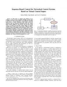
Baseline tracking response with minimal delay n(t) 6= 0.

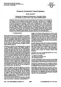
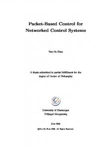
controller yc (j) = kc ec (j) in which the gain kc is chosen to satisfy the conditions in Corollary 1 such that √ −ǫ2 ap = 1 1 2 ǫ τ < kc < τ = − ap . In addition KM Ts = M Ts is chosen so that rs (j) = yp (t) at steady-state. Fig. 6 depicts a classic digital position feedback control scheme in which rc (j) = yp−classic (jM Ts ) at steady-state when n(t) = 0. In order to compare the effects of band-limited noise n(t), the low-pass filtered and noise-corrupted feedback signal ynp (j) is periodically sampled every M Ts seconds for the classical scheme whereas the signal yp depicted in Fig. 1 is corrupted similarly such that yp (t) = (Hp ep (t) + n(t)). For our high-performance system we filter the noise corrupted signal using the multi-rate passive sampler subsystem (Fig. 5) 1 . In described in Section III-B in which HLPc (s) = τ s+1 addition a second stage digital anti-aliasing filter HLP (z) was synthesized by applying the IPESH-Transform to a sixth order low-pass Butterworth filter model HLP (s) with passband ωp = MπTs [22, Section 9.7.5]. The simulation parameters are as follows: ǫ = 2, Mp = 2 M Ts .4 kg, Ts = .01 seconds, M √ = 10, τ = π , π < kc = 3 < 10π and KM Ts = M Ts . Fig. 7 indicates that our high-performance position yp (t) response tracks the desired reference rs (j) closer than the classic digital control system response yp−classic (t) when subject to band-limited noise within the frequency band [ MπTs , Tπs ]. Finally, Fig. 8 indicates that our proposed system is significantly less sensitive to the introduction of a 0.5 second delay between the controller and the plant.

IV. CONTROLLER VALIDATION & SIMULATION Next, we validate our results through the control of an idealized single degree of freedom haptic paddle as described in Section II and depicted in Fig. 2. This nominal plant system Hp (s) will be controlled using our digital control network depicted in Fig. 1 in which we shall use a proportional

V. APPLICATION FOR TELEMANIPULATION The Novint Falcon [28] is a low cost haptic interface which provides a 10 cm × 10 cm × 10 cm workspace providing position information ypl ∈ R3 while allowing for up to a 10 N force input eMpl ∈ R3 to be applied to the user in each

8

1.5

r (j) s

y

(t)

p−classic

y (t)

1

p

position (m)

0.5

0

−0.5

−1

−1.5 10

Fig. 8.

15

20 t (s)

25

30

Position response with 0.5 second delay.

Fig. 11.

Fig. 9.

Haptic Paddle Dynamics Hpl : epl → ypl .

of the three directions. Although the kinematics are quite complex [29] the standard drivers provided by Novint and standard Simulink interface provided by the Haptik Library [30] adequately allow us to model the haptic interface as a three dimensional point mass system. As was previously discussed for the single input-output point mass system applies to the three dimensional systems Hpl : epl → ypl l ∈ {1, 2} with filtered velocity compensation depicted in Fig. 9. In order to simplify discussion we ignore the effects of gravity which can be compensated for by either i) the human operator, ii) adding an appropriate bias term to rc (j) for the telemanipulation control subsystem Hc : ec → yc , T T T T T 3 ec = [eT c1 , ec2 ] , yc = [yc1 , yc2 ] , ecl , ycl ∈ R depicted in Fig. 10 or iii) adding gravity compensation directly to each paddle subsystem Hpl . The role of the controller is to make yp1 = yp2 and eMp1 = −eMp2 while satisfying the constraints required by Corollary 1 which are sufficient for stability. We therefore choose to couple each plant Hpl : epl → ypl T T subsystem such that Hp : ep → yp in which ep = [eT p1 , ep2 ] T T T and yp = [yp1 , yp2 ] . It is obvious that such a coupling can be accomplished with either one or two synchronized embedded controllers since the inputs and outputs are in parallel. In addition the control subsystem can be implemented on either a shared or an entirely separate embedded controller in which data between each devices can be exchanged using wave

Fig. 10.

Telemanipulation Controller Hc : ec → yc .

Experimental Setup for Telemanipulation

variables and subjected to appropriately handled time delays and data loss without adversely affecting stability. The control subsystem depicted in Fig. 10 is designed such that Hc : ec → yc is inside the sector c ]. This  [ac , b I I is an can be verified by noting that: R = √12 −I I T orthogonal matrix such that R R = I. Using Theorem 4 in Appendix II we can verify  that the intermediate maac +bc I 0 2 trix Kc = is inside the sector [ac , bc ]. 2ac bc 0 ac +bc I Specifically Kc can be thought of two subsystems in which √c1 (ec1 − ec2 ) is inside the sector HKc1 : √12 (ec1 − ec2 ) → K 2 ac +bc ac +bc √c2 (ec1 + ec2 ) [ 2 , 2 ] and HKc2 : √12 (ec1 + ec2 ) → K 2 ac +bc 2ac bc 2ac bc c bc is inside the sector [ ac +bc , ac +bc ]. We choose 2 > a2a c +bc in order to make ypd1 ≈ ypd2 (rc = 0) (Ideally ac = 0 however if ap < 0 then we will need some minimal feedthrough). Therefore a + b = 2(ac2+bc ) = ac + bc and 4(ac bc )2 (ac +bc ) a c bc ab a+b = 4ac bc (ac +bc )2 = ac +bc . Finally, from Theorem 5 in Appendix II since R is an orthogonal matrix then RKc RT is inside the sector [ac , bc ]. Fig. 11 shows an experimental setup designed for the application of the framework for telemanipulation. The experimental setup consists of two Novint Falcons, connected using a networked computing platform with one paddle acting as the “Leader” and the other the “Follower”. The computing platform consists of two networked Windows PCs with Matlab/Simulink. The haptic paddles are each connected to two respective PCs via USB interface utilizing Matlab/Simulink APIs. The haptic paddle API also enables a user to feel the feedback of forces and this in a sense enables transparency. In the setup, the “Follower” runs on one of the PCs denoted “Follower PC” and the “Leader” paddle runs on the other PC. The controller described in Fig. 10 is implemented as a Simulink model and runs on the same PC as the “Leader” paddle.

9

VI. CONCLUSIONS 0.06 0.04

Position(meters)

0.02 0 −0.02 −0.04 −0.06 Follower x−position Leader x−position

−0.08 −0.1 30

Fig. 12.

40

50 time (sec)

60

70

Plot of Leader and Follower paddles’ x-position

In [30], the authors described the sampling rate limitation in accessing the position information from the haptic paddles. Due to this limitation, a continuous signal of the position can not be obtained through the haptic paddle interface therefore the multi-rate passive sampler (PS : M Ts ) and passive hold (PH : M Ts ) are not used. Instead, the experiment was carried out using discrete-time the wave variables and the passive upsampler (PUS : M ) and passive downsampler (PDS : M ) as described in [3]. Through a series of experiments, the passive upsampler and passive downsampler were evaluated and it was noticed that the apparent stiffness in controlling the “Follower” manipulator decreases as we increase M . Hence, using a small M allows for a better control of the “Follower” manipulator. The sampling time,Ts , of 0.04 seconds was used in the course of the experiment. The other parameters for the experiment are as follows: M = 1, Mp = 0.164kg, b = 1, (b2 )∗2∗T s p∗π π , bc = (2∗T τ = MπTs , Kp = M 2∗T s , ac = π s) . During the course of the experiments, it was observed that the paddles experience a large amount of friction which limits tracking performance. In order to improve performance without adversely affecting stability, the input to the haptic paddle systems paddle,epl is amplified by a value of 4 before sending it to the haptic paddle systems. In a typical operation using this setup, when a paddle is moved the position signal in x-y-z coordinates is sent to a Matlab/Simulink haptic paddle interface block. This signal is then transformed into wave variables and then sent to the controller. The controller, using the position information from both paddles, calculates the required control signal needed to maintain position tracking. The computed control signal is sent as wave variables over the network to the “Follower” paddle and locally to the “Leader” paddle. Fig. 12 shows a plot of the x-positions of the “Leader” and “Follower” paddles after a trial run. From the figure, it can be seen that the “Follower” paddle closely tracks the position of the “Leader” paddle. Also, from the plot there is slight discernible difference between the positions of the “Leader” and “Follower” paddles. This can be attributed to the excessive friction in the paddles which slightly affects tracking performance.

We have provided a set of sufficient conditions to guarantee delay independent stability for non-passive systems Hp inside the sector [ap , bp ] −∞ < ap < bp for our networked control architecture depicted in Fig. 1. In particular, Theorem 1 and Assumption 1 allow us to derive Theorem 2 which describe the internal network structure depicted in Fig. 4. Lemma 1 shows that a linear passive sampler depicted in Fig. 5 satisfied the key inequality (12). As a result linear anti-aliasing filters can be introduced which do not adversely affect stability or performance. Lemma 2 and Corollary 1 provide the sufficient sector conditions for the controller and plant to achieve the small gain conditions required of Theorem 3 in order to guarantee Lm 2 -stability. Corollary 2 shows that the IPESH-Transform can be applied to an analog controller to synthesize a digital controller such that both controllers are inside the sector [a, b]. Simulation results of our proposed architecture applied to direct position control of a haptic paddle indicate good performance with low sensitivity to band-limited noise and networked delay. R EFERENCES [1] P. J. Antsaklis and J. Baillieul, Eds., Special Issue: Technology of Networked Control Systems. Proceedings of the IEEE, 2007, vol. 95 no. 1. [2] N. Kottenstette, X. Koutsoukos, J. Hall, J. Sztipanovits, and P. Antsaklis, “Passivity-Based Design of Wireless Networked Control Systems for Robustness to Time-Varying Delays,” Real-Time Systems Symposium, 2008, pp. 15–24, 2008. [3] N. Kottenstette, J. F. Hall, X. Koutsoukos, P. Antsaklis, and J. Sztipanovits, “Digital control of multiple discrete passive plants over networks,” International Journal of Systems, Control and Communications (IJSCC), no. Special Issue on Progress in Networked Control Systems, 2011, to Appear. [4] C. A. Desoer and M. Vidyasagar, Feedback Systems: Input-Output Properties. Orlando, FL, USA: Academic Press, Inc., 1975. [5] G. Niemeyer and J.-J. E. Slotine, “Telemanipulation with time delays,” International Journal of Robotics Research, vol. 23, no. 9, pp. 873 – 890, 2004. [6] R. Anderson and M. Spong, “Asymptotic stability for force reflecting teleoperators with time delay,” The International Journal of Robotics Research, vol. 11, no. 2, pp. 135–149, 1992. [7] N. Kottenstette and P. Antsaklis, “Relationships between positive real, passive dissipative, & positive systems,” American Control Conference, pp. 409–416, 2010. [8] G. Zames, “On the input-output stability of time-varying nonlinear feedback systems. i. conditions derived using concepts of loop gain, conicity and positivity,” IEEE Transactions on Automatic Control, vol. AC-11, no. 2, pp. 228 – 238, 1966. [9] J. C. Willems, The Analysis of Feedback Systems. Cambridge, MA, USA: MIT Press, 1971. [10] N. Kottenstette and J. Porter, “Digital passive attitude and altitude control schemes for quadrotor aircraft,” Dec. 2009, pp. 1761 –1768. [11] N. Kottenstette and N. Chopra, “Lm2-stable digital-control networks for multiple continuous passive plants,” 1st IFAC Workshop on Estimation and Control of Networked Systems (NecSys’09), 2009. [12] S. Hirche and M. Buss, “Transparent Data Reduction in Networked Telepresence and Teleaction Systems. Part II: Time-Delayed Communication,” Presence: Teleoperators and Virtual Environments, vol. 16, no. 5, pp. 532–542, 2007. [13] N. Chopra, P. Berestesky, and M. Spong, “Bilateral teleoperation over unreliable communication networks,” IEEE Transactions on Control Systems Technology, vol. 16, no. 2, pp. 304–313, 2008. [14] S. Hirche, T. Matiakis, and M. Buss, “A distributed controller approach for delay-independent stability of networked control systems,” Automatica, vol. 45, no. 8, pp. 1828–1836, 2009.

10

Fig. 13. Plant-rp -vp -yp -up -network realization and initial transformation.

[15] M. Kuschel, P. Kremer, and M. Buss, “Passive haptic data-compression methods with perceptual coding for bilateral presence systems,” IEEE Transactions on Systems, Man and Cybernetics, Part A: Systems and Humans, vol. 39, no. 6, pp. 1142 – 1151, Nov. 2009. [16] D. J. Hill, “Dissipative nonlinear systems: Basic properties and stability analysis,” Proceedings of the 31st IEEE Conference on Decision and Control, pp. 3259–3264, 1992. [17] D. J. Hill and P. J. Moylan, “The stability of nonlinear dissipative systems,” IEEE Transactions on Automatic Control, vol. AC-21, no. 5, pp. 708 – 11, 1976. [18] ——, “Stability results for nonlinear feedback systems,” Automatica, vol. 13, pp. 377–382, 1977. [19] G. C. Goodwin and K. S. Sin, Adaptive Filtering Prediction and Control. Englewood Cliffs, New Jersey 07632: Prentice-Hall, Inc., 1984. [20] W. M. Haddad and V. S. Chellaboina, Nonlinear Dynamical Systems and Control: A Lyapunov-Based Approach. Princeton, New Jersey, USA: Princeton University Press, 2008. [21] R. J. Anderson and M. W. Spong, “Bilateral control of teleoperators with time delay,” Proceedings of the IEEE Conference on Decision and Control Including The Symposium on Adaptive Processes, pp. 167 – 173, 1988. [22] A. Oppenheim, A. Willsky, and S. Nawab, Signals and systems. Prentice hall Upper Saddle River, NJ, 1997. [23] N. Kottenstette and P. Antsaklis, “Wireless Control of Passive Systems Subject to Actuator Constraints,” 47th IEEE Conference on Decision and Control, 2008. CDC 2008, pp. 2979–2984, 2008. [24] S. Stramigioli, C. Secchi, A. J. van der Schaft, and C. Fantuzzi, “Sampled data systems passivity and discrete port-hamiltonian systems,” IEEE Transactions on Robotics, vol. 21, no. 4, pp. 574 – 587, 2005. [25] J.-H. Ryu, Y. S. Kim, and B. Hannaford, “Sampled- and continuoustime passivity and stability of virtual environments,” IEEE Transactions on Robotics, vol. 20, no. 4, pp. 772 – 6, 2004. [26] N. Kottenstette and P. Antsaklis, “Stable digital control networks for continuous passive plants subject to delays and data dropouts,” 46th IEEE Conference on Decision and Control, pp. 4433–4440, 2007. [27] G. F. Franklin, J. D. Powell, and A. Emami-Naeini, Feedback Control of Dynamic Systems, 5th ed. Prentice-Hall, 2006. [28] NOVINT Falcon. [Online]. Available: http://home.novint.com/ products/novint falcon.php [29] S. Martin and N. Hillier, “Characterisation of the novint falcon haptic device for application as a robot manipulator,” Australasian Conference on Robotics and Automation (ACRA), pp. 1–9, 2009. [30] M. de Pascale and D. Prattichizzo, “The Haptik Library: a component based architecture for uniform access to haptic devices,” IEEE Robotics and Automation Magazine, vol. 14, no. 4, pp. 64–75, 2007. [31] J. T. Wen and M. Arcak, “A unifying passivity framework for network flow control,” IEEE Transactions on Automatic Control, vol. 49, no. 2, pp. 162 – 174, 2004. [Online]. Available: http://dx.doi.org/10.1109/TAC.2003.822858

A PPENDIX I WAVE VARIABLE N ETWORK P ROPERTIES Fig. 13 depicts a graphical realization of (7) on the lefthand-side (LHS), and the first obvious graphical transformation on the right-hand-side (RHS) in which we denote closed-loop transformation of the plant Hp in terms of the feedback gain ǫ as Hclp : eclp → yp in which √ (29) eclp (t) = rp (t) + 2ǫvp (t) = ep (t) + ǫyp (t).

Fig. 14.

Final Plant-rp -vp -yp -up -network realization.

Fig. 15. mation.

Controller-rc -uc -ep -vc -network realization and initial transfor-

In order to simplify discussion and to leverage Theorem 1 we use Assumption 1 in order to derive Corollary 3: Corollary 3: If Assumptionh 1 is satisfied i then Hclp : bp ap . , eclp → yp is inside the sector 1+ǫa p 1+ǫbp Next we transform the RHS realization in Fig. 13 to the final form depicted in Fig. 14. Lemma 4: The RHS of Fig. 13 can be transformed to the in Fig. 14 (in which Hpe eclp = √ final form depicted 2ǫHclp eclp − √12ǫ eclp ). In addition if Assumption 1 is satish i √ ǫa −1 ǫb −1 fied, then 2ǫHpe eˆclp (t) is inside the sector ǫapp +1 , ǫbpp +1 . Proof: From Fig. 14 it is clear that,   √ √ 1 eclp (t) = 2ǫ √ rp (t) + vp (t) = rp (t) + 2ǫvp (t) 2ǫ which satisfies (29), next from Fig. 14 it is clear that, √ 1 1 up (t) = 2ǫyp (t) − √ eclp (t) + √ rp (t) 2ǫ 2ǫ  √ √ 1  1 = 2ǫyp (t) − √ rp (t) + 2ǫvp (t) + √ rp (t) 2ǫ 2ǫ √ = 2ǫyp (t) − vp (t). which satisfies (7) in regards to up (t). From Corollary 3 we h have thati Hclp : eclp → yp is inside the sector ap bp 1+ǫap , 1+ǫbp . From the scaling property (Property 1-iv), √ √ √ we have that Hclph 2ǫ = 2ǫHclp in iwhich 2ǫHclp is √ √ ap bp , 2ǫ 1+ǫb . Using the sum inside the sector 2ǫ 1+ǫa p p ruleh (Property 1-v) we have that Hpei is inside the sec√ √ ap bp −1 √ + + tor √−1 2ǫ 2ǫ 1+ǫb , solving for ape we 1+ǫa p p 2ǫ 2ǫ  √ ap 2ǫap −ǫap −1 √1 2ǫ + = therehave ape = √−1 1+ǫaph 2ǫ 2ǫ ǫap +1  i ǫap −1 ǫbp −1 1 1 fore Hpe is inside the sector √2ǫ ǫap +1 , √2ǫ ǫbp +1 √ finally from the hscaling property i we have that 2ǫHpe is ǫa −1 ǫb −1 inside the sector ǫapp +1 , ǫbpp +1 . Fig. 15 depicts a graphical realization of (8) on the left-handside (LHS), and the first obvious graphical transformation on the right-hand-side (RHS) in which we denote closed-loop

11

Fig. 16.

Final Controller-rc -uc -yc -vc -network realization.

transformation of the controller Hc in terms of the feedback gain 1ǫ as Hclc : eclc → yc in which r 2 1 uc (j) = ec (j) + yc (j). (30) eclc (j) = rc (j) + ǫ ǫ Which allows us to state the following corollary: Corollary 4: If Assumptionh 1 is satisfied then Hclc : i ǫac ǫbc eclc → yc is inside the sector ǫ+ac , ǫ+bc . Next we transform the RHS realization in Fig. 15 to the final form depicted in Fig. 16. Lemma 5: The RHS of Fig. 15 can be transformed to theqfinal form depicted in Fig. 16 (in which Hce eclc = p − 2ǫ Hclc eclc + 2ǫ eclc ). In addition if Assumption 1 is satq h i c ǫ−ac isfied, then 2ǫ Hce eˆclc (j) is inside the sector ǫ−b ǫ+bc , ǫ+ac . Proof: From Fig. 16 it is clear that, r r r  2 ǫ 2 rc (j) + uc (j) = rc (j) + uc (j) eclc (j) = ǫ 2 ǫ

Fig. 17.

Concatenation of m conic systems H : u → y.

r

2 Hce is inside the sector ǫ



 ǫ − bc ǫ − a c . , ǫ + bc ǫ + a c

A PPENDIX II A DDITIONAL P ROPERTIES OF C ONIC S YSTEMS Fig. 17 depicts a concatenation of m conic systems Hl : ul → yl inside the sector [al , bl ] in which 0 ≤ |al |, bl < ∞, T T T T T (bl + al ) > 0, u = [uT 1 , . . . , um ] and y = [y1 , . . . , ym ] , l ∈ {1, . . . , m} which we denote H : u → y. Theorem 4: The concatenated system H : u → y depicted in Fig. 17 is inside the sector [a, b] in which:

a + b = max{al + bl } ab a l bl which satisfies (30), next from Fig. 16 it is clear that, = min{ } ∀ l ∈ {1, . . . , m} a + b a + bl l r r r Pm 2 ǫ ǫ Vl (xl ). and V (x) = l=1 aa+b yc (j) + eclc (j) − rc (j) vc (j) = − l +bl ǫ 2 2 Proof: Assuming each subsystem Hl : ul → yl is a ! r r r r conic-dissipative system in which 0 < (bl + al ) < ∞ we 2 ǫ 2 ǫ =− rc (j) + yc (j) + uc (j) − rc (j) have that ǫ 2 ǫ 2 r 1 a l bl 2 hyl , ul iT ≥ k(yl )T k22 + k(ul )T k22 yc (j) + uc (j). =− a l + bl a l + bl (31) ǫ 1 (V (x (T )) − V (x (0))) . + l l l l which satisfies (8) in regards to vc (j). From Corollary 4 a l + bl hwe have that i Hclc : eclc → yc is inside the sector Summing both sides of (31) w.r.t. l ∈ {1, . . . , m} results in: ǫac ǫbc ǫ+ac , ǫ+bc . From the scaling property, we have that q q q m  X 1 a l bl −Hclc 2ǫ = − 2ǫ Hclc in which − 2ǫ Hclc is inside the hy, uiT ≥ k(yl )T k22 + k(ul )T k22 q q h i a l + bl a l + bl l=1 ǫbc ǫac  sector − 2ǫ ǫ+b . Using the sum rule we have , − 2ǫ ǫ+a c c 1 (Vl (xl (T )) − Vl (xl (0))) . + that a l + bl a l bl 1 Hce is inside the sector k(y)T k22 + min{ }k(u)T k22 ≥ "r # r r r max{a + b } a + b l l l l ǫ 2 ǫbc ǫ 2 ǫac m − , − X 1 2 ǫ ǫ + bc 2 ǫ ǫ + ac (Vl (xl (T )) − Vl (xl (0))) + a l + bl l=1 solving for bce we have r r  r  1 ab 2ac ǫ 2 ǫac ǫ ≥ k(y)T k22 + k(u)T k22 1− − = bce = a+b a+b 2 ǫ ǫ + ac 2 ǫ + ac 1 [V (x(T )) − V (x(0))] . + therefore Hce is inside the sector a + b r   r   ǫ ǫ − bc ǫ ǫ − ac The proof for the discrete-time case follows analogously. , 2 ǫ + bc 2 ǫ + ac Fig. 18 consists of orthogonal matrices RT and R (RT R = I) and a conic-dissipative system H : RT u → y which is finally from the scaling property we have that

12

Fig. 18. Orthogonal matrices RT R = I preserve conic properties of H : RT u → y.

inside the sector [a, b]. For the more general case when R is simply a full column rank matrix that passivity is always conserved as is done for passivity based network flow control problems [31]. However, in order to preserve the overall conic properties of the system we need to restrict the matrices to be orthogonal. Theorem 5: If the matrix R is an orthogonal matrix (RT R) then H : RT u → y is a conic-dissipative system inside the sector [a, b] iff HR : u → Ry is inside the sector [a, b]. Proof: Since uT RT Ru = uT u and if H : RT u → y is inside the sector [a, b] then ( −y T y + (a + b)y T RT u − abuT u, |a|, |b| < ∞ T s(R u, y) = y T RT u − auT u, |a| < ∞, b = ∞. Next we assume that HR : u → Ry is inside the sector [¯ a, ¯b] T T T and since y R Ry = y y then: ( −y T y + (¯ a + ¯b)y T RT u − a ¯¯buT u, |¯ a|, |¯b| < ∞ s(u, Ry) = y T RT u − a ¯uT u, |¯ a| < ∞, ¯b = ∞. Since s(u, Ry) = s(RT u, y) if a ¯ = a and ¯b = b then HR : u → Ry is inside the sector [a, b]. Necessity can be easily shown by changing the order of assumptions.