Networked Control of Distributed Energy Systems

Networked Control of Distributed Energy Systems By ASHRAF F. KHALIL

A Thesis Submitted To The University Of Birmingham For The Degree Of DOCTOR OF PHILOSOPHY

School Of Electronic, Electrical & Computer Engineering College Of Engineering & Physical Science The University Of Birmingham, UK February 2012

University of Birmingham Research Archive e-theses repository This unpublished thesis/dissertation is copyright of the author and/or third parties. The intellectual property rights of the author or third parties in respect of this work are as defined by The Copyright Designs and Patents Act 1988 or as modified by any successor legislation. Any use made of information contained in this thesis/dissertation must be in accordance with that legislation and must be properly acknowledged. Further distribution or reproduction in any format is prohibited without the permission of the copyright holder.

DECLARATION

I confirm that the work in this which is thesis entitled “Networked Control of Distributed Energy Systems”, is my own work.

Ashraf Khalil

ABSTRACT

Networked control systems have attracted a great attention in the last decade, and their applications in distributed energy systems have been addressed by many researchers. Replacing the complex wiring system with a shared network can improve the system performance, reliability and stability. When a shared network is adopted in the control loops, the control signals will suffer time delays or data dropouts which may destabilize the system. So it is necessary to find the maximum time delay that the system can withstand. The methods available in the literature either are an extension from those designed for time delay systems or are too complex to be used in practice. This thesis reports a new method for stability analysis and maximum time delay estimation in networked control systems with applications to distributed energy systems. The proposed new method is based on using finite difference approximation for the delay term and then the Lyapunov system stability theorem is applied to derive the time delay boundary allowed to the system. The proposed method has been applied to networked control systems with state feedback controllers, with dynamic controllers, and to multi-units interconnected networked control systems. The proposed method is then extended to a class of networked control system with bounded nonlinearity and uncertainties. Compared with most of the methods reported in the published literature, the new method is simple to use while the results are comparable. The characteristics of time delays are analyzed in this thesis, and the results show that time delays can be constant, periodic, random and bounded, random governed by Markov Chain and in some cases the time delay may be unbounded. The proposed method

i

is suitable for systems with bounded time delays which is required in networked control systems. The method is applied to analyze the stability of a system with parallel connections of DC/DC buck converters where the control signals are exchanged through the shared network. With the proposed method, the parameters that affect the maximum allowable delay boundary are investigated. When the time delay can be modelled using Markov Chain the Markovian jump system approach is used to study the stability of the networked control system. With this approach, the stability of the networked control system is formulated as finding the solutions for a Bilinear Matrix Inequality. In this thesis, an improved V-K iteration algorithm is used to solve the Bilinear Matrix Inequality in order to derive a controller to stabilize the systems. This approach is used to study the stability of the parallel DC/DC converters with stochastic time delays. The proposed method is extended for a class of nonlinear networked control systems and uncertain networked control systems. This extension has resulted in two theorems to determine the stability of such a networked control system. The method supported by the theorem for the nonlinear networked control system involves less computation compared with the methods published in the literature, and the designed controller has established the relationship between the maximum allowable delay bound and the maximum nonlinearity. It is found that increasing the nonlinearity in the system will result in decreasing the maximum allowable time delay. The proposed method in this thesis is simple in structure and applications with comparable performance to most of the published methods in the literature. With the increase reliance on shared networks in industry and distributed energy systems in control engineering practice the method can be used as a fast and simple design tool. ii

ACKNOWLEDGEMENT

I am grateful to Allah the Almighty who gives me all what I need, who guides and helps me during my journey in this life. I would like to express my gratitude to my supervisor Prof. Jihong Wang, who guided me during my research, and I appreciate her patience and advice. Her encouragement and support were really great motivation for me. I really have benefited from each minute of discussion with Prof. Jihong Wang. The suggestions, criticisms and the guidance I received from her were valuable, which made this thesis possible. To Dr. Mourad Oussalah and Dr. Stuart Hillmansen thank you for your suggestions and criticisms. The comments which I received from Dr. Mourad were very important for improving this work. I am really grateful for the scholarship I received from the ministry of the higher education in Libya. Thanks to my parents, brothers, sisters and friends for their encouragement and support. I am really grateful to my wife for her patience during my research. I would like to thank her for the endless love and support. And finally to her and my kids Mouhanad, Khalid, Sondes and Malik I dedicate my thesis.

iii

Table of Contents CHAPTER ONE: INTRODUCTION................................................................................1 1.1 MOTIVATION OF THE RESEARCH ................................................................................................... 2 1.2 REVIEW OF THE PREVIOUS RESEARCH IN NCSS................................................................................... 6 1.3 DESCRIPTION OF NETWORKED CONTROL SYSTEMS..............................................................................12 1.3.1 Network-Induced Delays in Networked Control System ......................................................16 1.3.2 Packets Dropouts: ......................................................................................................17 1.3.3 NCSs Structures: .........................................................................................................18 1.3.4 Networked Control System Stability: ..............................................................................19 1.4 MAIN CONTRIBUTIONS OF THE THESIS ...........................................................................................21 1.5 THESIS OUTLINE ......................................................................................................................................... 24 1.6 SUMMARY..........................................................................................................................26

CHAPTER TWO: TIME DELAYS IN SHARED NETWORKS .................................27 2.1 INTRODUCTION ....................................................................................................................27 2.2 TIME DELAYS.......................................................................................................................28 2.2.1 Network Schedule.......................................................................................................29 2.2.2 Network Utilization .....................................................................................................29 2.3 CONTROL NETWORKS .............................................................................................................30 2.3.1 Controller Area Network (CAN) .....................................................................................31 2.3.2 Ethernet ...................................................................................................................32 2.4 TRUETIME 1.5 SIMULATOR .......................................................................................................34 2.5 SIMULATION RESULTS FOR THE CAN AND THE ETHERNET ......................................................................35 2.5.1 The Time Delay Analysis in the CAN................................................................................35 2.5.2 The Time Delay Analysis in the Ethernet ..........................................................................47 2.6 DISCUSSIONS .......................................................................................................................52 2.7 SUMMARY..........................................................................................................................54

CHAPTER 3: MAXIMUM ALLOWABLE DELAY ESTIMATION FOR NETWORKED CONTROL SYSTEMS..........................................................................55 3.1 INTRODUCTION ....................................................................................................................55 3.2 TIME DELAYS IN NETWORKED CONTROL SYSTEMS................................................................................56 3.3 MAXIMUM ALLOWABLE DELAY BOUND ESTIMATION FOR NCSS ................................................................59 3.3.1 The mathematical model of a single unit NCS ..................................................................59 3.3.2 Maximum allowable delay bound estimation in the time domain ........................................61 3.3.3 Maximum allowable delay bound estimation in the s-domain .............................................65 3.3.4 Numerical examples for estimating the maximum allowable delay bound .............................69 3.4 MAXIMUM ALLOWABLE DELAY BOUND ESTIMATION FOR NCSS WITH DYNAMIC CONTROLLERS ..............................74 3.4.1 The mathematical model of NCSs with dynamic controllers ................................................74 3.4.2 Case I: Neglecting τ ca .................................................................................................75 3.4.3 Case II: Taking τ ca into consideration: .............................................................................78 3.4.4 Maximum allowable delay bound estimation in the s-domain .............................................79 3.5 CONTROLLER DESIGN USING THE FINITE DIFFERENCE APPROXIMATION: ........................................................84 3.6 NETWORKED CONTROL OF DISTRIBUTED INTERCONNECTED UNITS ............................................................87 3.6.1 Mathematical model of n-connected networked control systems .........................................88 3.6.2 Example: A three synchronous generators controlled over network ......................................91 3.7 SUMMARY..........................................................................................................................99

iv

CHAPTER 4: ROBUST STABILIZATION OF NETWORKED CONTROL SYSTEM USING MARKOVIAN JUMP SYSTEM APPROACH .............................100 4.1 INTRODUCTION .................................................................................................................. 100 4.2 JUMP LINEAR SYSTEMS .......................................................................................................... 101 4.3 MATHEMATICAL MODELLING OF NCSS WITH TIME DELAY ................................................................... 106 4.3.1 Modelling of a Class of Networked Control Systems ........................................................ 106 4.3.2 Modelling Time Delays Using Markov Chains ................................................................. 111 4.4 THE STABILITY OF LINEAR JUMP SYSTEM ....................................................................................... 112 4.5 THE V-K ITERATION ............................................................................................................. 114 4.5.1 The Feasibility Problem (FP) ........................................................................................ 116 4.5.2 The Eigenvalue Problem (EVP) .................................................................................... 116 4.5.3 The Generalized Eigenvalue Problem (GEVP) .................................................................. 118 4.5.4 The V-K Iteration Algorithm: ....................................................................................... 120 4.6 EXAMPLE 4.1: THE CART AND INVERTED PENDULUM: ........................................................................ 123 4.7 SUMMARY........................................................................................................................ 131

CHAPTER FIVE: NETWORKED CONTROL OF PARALLEL DC/DC BUCK CONVERTERS................................................................................................................132 5.1 INTRODUCTION: ................................................................................................................. 132 5.2 PARALLEL DC/DC BUCK CONVERTERS ......................................................................................... 135 5.2.1 The Parallel DC/DC Buck Converters Mathematical Model ................................................ 135 5.2.2 The Controller Model ................................................................................................ 137 5.3 NETWORKED CONTROL OF PARALLEL DC/DC CONVERTERS WITH CONSTANT TIME DELAY ............................... 139 5.4 NETWORKED CONTROL OF THE PARALLEL DC/DC CONVERTERS WITH RANDOM TIME DELAY GOVERNED BY MARKOV CHAINS ................................................................................................................................ 144 5.5 CASE STUDY: THREE PARALLEL DC/DC CONVERTERS ........................................................................ 146 5.5.1 Networked control of parallel DC/DC buck converter with the constant time delay model:...... 148 5.5.2 Networked Control with Constant Time Delay ................................................................ 157 5.5.3 Networked Control with Periodic Time Delay ................................................................. 160 5.5.4 Networked Control with Independent Random Time Delay ............................................... 163 5.5.5 Networked Control withRandom Time Delay Governed by Markov Chain: ........................... 167 5.6 SUMMARY........................................................................................................................ 176

CHAPTER SIX: TIME DELAY TOLERANCE ESTIMATION FOR A CLASS OF NONLINEAR AND UNCERTAIN NETWORKED CONTROL SYSTEMS ...........177 6.1 INTRODUCTION .................................................................................................................. 177 6.2 RECENT STUDY ON NONLINEAR NETWORKED CONTROL SYSTEMS WITH TIME DELAYS ..................................... 178 6.3 STABILITY OF A CLASS OF NONLINEAR NETWORKED CONTROL SYSTEMS: ..................................................... 180 6.3.1 Mathematical Model of Networked Control System with Nonlinearity ................................ 180 6.3.2 Estimation of Domain of Attraction .............................................................................. 187 6.3.3 Examples of applications............................................................................................ 189 6.4 STABILITY OF UNCERTAIN NETWORKED CONTROL SYSTEM ................................................................... 200 6.4.1 Mathematical Model of Uncertain Networked Control System .......................................... 201 6.4.2 Examples of Applications ........................................................................................... 205 6.5 SUMMARY........................................................................................................................ 209

CHAPTER SEVEN: CONCLUSIONS AND FUTURE WORK.................................210 7.1 MAIN CONCLUSIONS ............................................................................................................ 210 7.2 SUGGESTED FUTURE WORK .................................................................................................... 215

REFERENCES.................................................................................................................216 APPENDIX A...................................................................................................................228

v

List of Figures Figure 1.1 A Fully Centralized Controller ......................................................................... 4 Figure 1.2 A Decentralized Control System ....................................................................... 4 Figure 1.3 A Quasi-Centralized Control System ................................................................ 5 Figure 1.4 The AGC with bilateral contract (Bhowmik et al. 2004). .................................. 8 Figure 1.5 A Typical Networked Control System ............................................................ 13 Figure 1.6 Time Delay in NCS ........................................................................................ 16 Figure 1.7 Packets Dropouts in NCS ............................................................................... 17 Figure 1.8 Packets out-of-order in NCS ........................................................................... 18 Figure 1.9 (a) Direct Structure of NCS, (b) Hirarchical Structure of NCS ........................ 19 Figure 2.1 The message frame format of CAN (Lian et al. 2001) ..................................... 32 Figure 2.2 The message frame format of Ethernet (Lian et al. 2001) ................................ 33 Figure 2.3 The TrueTime Block Library. ......................................................................... 34 Figure 2.4 The CAN with seven nodes ............................................................................ 36 Figure 2.5 The time delay in the CAN with low load, solid-line 94 bit message, dashed-line 128 bit message. .............................................................................................................. 37 Figure 2.6 The Network Schedule ................................................................................... 38 Figure 2.7 The time delay with periodic load messages ................................................... 39 Figure 2.8 The network schedule with periodic messages load. ....................................... 40 Figure 2.9 The time delay with random messages and middle priority ............................. 42 Figure 2.10 The histogram of the time delay in Figure 2.9 ............................................... 42 Figure 2.11 The network schedule with random messages load. ...................................... 43 Figure 2.12 The time delay with random messages and middle priority and 0.012 s load message ........................................................................................................................... 44 Figure 2.13 The histogram of the time delay in Figure 2.12 ............................................. 44 Figure 2.14 The network schedule with random messages load. ...................................... 45 Figure 2.15 The time delay with random messages and middle priority with 0.009 s load message ........................................................................................................................... 46

vi

Figure 2.16 The histogram of the time delay in Figure 2.15 ............................................. 46 Figure 2.17 The network schedule with random messages load. ...................................... 47 Figure 2.18 The Ethernet with seventeen nodes ............................................................... 48 Figure 2.19 The time delay in the Ethernet with low load ................................................ 49 Figure 2.20 The network schedule in the Ethernet with low load ..................................... 49 Figure 2.21 The time delay in the Ethernet with medium load ......................................... 50 Figure 2.22 The histogram of the time delay in Figure 2.21 ............................................. 51 Figure 2.23 The time delay in the Ethernet with medium utilization ................................ 52 Figure 3.1 A Typical Networked Control System ............................................................ 57 Figure 3.2 An NCS with time delay between the sensor and the controller ...................... 60 Figure 3.3 A Networked Control System ......................................................................... 74 Figure 3.4 The response of the CH-47 with 0.0018 s time delay ...................................... 84 Figure 3.5 The system response with 0.2 s time delay. ..................................................... 87 Figure 3.6 A networked system consists of n sub-systems. .............................................. 89 Figure 3.7 Three synchronous generators controlled over network................................... 92 Figure 3.8 Three machine interconnected power system .................................................. 93 Figure 3.9 The rotor angle deviation of the first generator. .............................................. 96 Figure 3.10 The speed deviation of the first generator. .................................................... 96 Figure 3.11 The rotor angle deviation of the second generator. ........................................ 97 Figure 3.12 The speed deviation of the second generator. ................................................ 97 Figure 3.13 The rotor angle deviation of the third generator. ........................................... 98 Figure 3.14 The speed deviation of the third generator. ................................................... 98 Figure 4.1 An example of a Markov chain load modelling, the three network loads: low (L), medium (M), and high (H). pij where i, j ∈ U = {L, M , H } is the probability of the transition from mode i to j ............................................................................................. 103 Figure 4.2 The Networked Control System .................................................................... 106 Figure 4.3 Networked Control System with both time delays from the sensor to the controller and from the controller to the actuator are taking into account ....................... 109 Figure 4.4 The V-K iteration algorithm………………………………………………….122

vii

Figure 4.5 The cart and inverted pendulum .................................................................... 123 Figure 4.6 The Simulink implementation of example 4.1 ............................................... 126 Figure 4.7 (a) The random time delay, (b) The response of the system in example 4.1 without time delay compensation (c) The response with time delay compensation ......... 127 Figure 4.8 (a) The random time delay, (b) The response of the system in example 4.1 without time delay compensation (c) The response with time delay compensation ......... 128 Figure 4.9 (a) The random time delay, (b) The response of the system in example 4.1 without time delay compensation (c) The response with time delay compensation ......... 130 Figure 4.10 (a) The random time delay, (b) The response of the system in example 4.1 without time delay compensation (c) The response with time delay compensation ......... 131 Figure 5.1 A parallel DC/DC Buck Converter system. ................................................... 136 Figure 5.2 Master-slave control strategy for two DC/DC parallel converters.................. 137 Figure 5.3 The master controller with both voltage and current controller...................... 138 Figure 5.4 The parallel DC/DC converters communicating through control network. .... 141 Figure 5.5 The Simulink implementation of the parallel DC/DC converters ................... 148 Figure 5.6 The output voltage with different values of time delay .................................. 149 Figure 5.7 The master, slave (1) and slave (2) currents .................................................. 150 Figure 5.8 The Maximum allowable delay bound verses the voltage controller gain: dashed-line: the method in (Gu et al. 2003), solid-line: the proposed method ................. 153 Figure 5.9 The MADB for different values of the voltage controller gain ...................... 153 Figure 5.10 The Output Voltage Response with different voltage gains, ........................ 154 Figure 5.11 The MADB for different values of the output voltage feedback factor k...... 154 Figure 5.12 The Output Voltage Responses with different values of the output voltage feedback factors, k ......................................................................................................... 155 Figure 5.13 The MADB for different values of the load resistance ................................ 155 Figure 5.14 The Output Voltage Responses with different values of resistances ............ 156 Figure 5.15 The MADB as function of the output voltage feedback gain, k, and the voltage controller K v ................................................................................................................ 156 Figure 5.16 The parallel DC/DC converters controlled over CAN bus ........................... 158 Figure 5.17 The time delay in CAN with low load ......................................................... 158 Figure 5.18 The output Voltage of the system under low load CAN .............................. 159

viii

Figure 5.19 (dashed line): The master reference current at the sending node, (solid line): The reference current signal at the slave node. ............................................................... 160 Figure 5.20 The time delay with periodic messages in the CAN .................................... 161 Figure 5.21 The output Voltage of the system under low load CAN .............................. 162 Figure 5.22 (dashed line): The master reference current at the sending node, (solid line): the reference current signal at the slave node. ................................................................ 162 Figure 5.23 The Parallel DC/DC buck converter system controlled over Ethernet.......... 163 Figure 5.24 The Ethernet with seventeen nodes ............................................................. 164 Figure 5.25 The time delay in the Ethernet with seventeen nodes .................................. 165 Figure 5.26 The probability distribution function of the time delay in Figure 5.25 ......... 165 Figure 5.27 The output voltage of the system controlled over the Ethernet .................... 166 Figure 5.28 (dashed line): The master reference current at the sending node, (solid line): the reference current signal at the slave node ................................................................. 167 Figure 5.29 The random time delay between the master controller and the slaves controller ...................................................................................................................................... 168 Figure 5.30 The output voltage with random time delay and K v = 125 . ......................... 169 Figure 5.31 (dashed line): The master reference current at the sending node, (solid line): the reference current signal at the slave node. ................................................................ 169 Figure 5.32 The random time delay between the master controller and the slaves controller ...................................................................................................................................... 170 Figure 5.33 The output voltage with random time delay and K v = 125 . ......................... 171 Figure 5.34 The time delay from the master controller to the slaves controllers ............. 171 Figure 5.35 The histogram of the time delay in Figure 5.34 ........................................... 172 Figure 5.36 The random time delay generated by the transition probability, P ............... 173 Figure 5.37 The histogram of the network time delay generated by the TrueTime 1.5 simulator and the modelled random time delay .............................................................. 173 Figure 5.38 The output voltage of the system with K v = 250 and k = 5 ....................... 174 Figure 5.39 The output voltage of the system with K v = 225 and k = 2 ....................... 175 Figure 6.1 The region of attraction ................................................................................ 188 Figure 6.2 The system response with zero time delay (solid-line) and 0.2509 s time delay (dashed-line) ................................................................................................................. 191

ix

Figure 6.3 The MADB as a function of the nonlinearity bound using Theorem 6.1 ........ 191 Figure 6.4 The MADB as a function of the maximum nonlinearity bound using Theorem 6.1 ................................................................................................................................. 192 Figure 6.5 The system response with 0.03 s time delay and α = 3 ................................. 193 Figure 6.6 The system response with 0.0801 s time delay and α = 0 ............................. 194 Figure 6.7 The MADB as a function of the maximum nonlinearity bound using Theorem 6.1 ................................................................................................................................. 194 Figure 6.8 The system response with 0.04 s time delay and α = 3 ................................. 195 Figure 6.9 The response of the system in Example 6.3 with 0.15 initial condition.......... 198 Figure 6.10 The system response with 0.76 s time delay and 0.15 initial condition ........ 199 Figure 6.11 The system response with 0.76 s time delay and 0.5 initial condition. ......... 199 Figure 6.12 The uncertain NCS with 0.8356 s time delay, solid-line x1, dashed-line x2 .. 206 Figure 6.13 The uncertain NCS with 0.6667 s time delay, solid-line x1 and dashed-line x2. ...................................................................................................................................... 207 Figure 6.14 The uncertain system with 0.907 s time delay, solid-line x1 and dashed-line x2. ...................................................................................................................................... 208

x

List of Abbreviations AC ACE AGC AWSS BMI CAN CCL CSMA/AMP CSMA/CD DC DES DTMJLS EVP FIB FP GCE GEVP ICCI JLS LAN LQG LQR LMI MADB NCS PID PROFIBUS PSS SCADA UPS VSI

Alternating Current Area Control Error Automatic Gain Control Asymptotic Wide Sense Stationary Stability Bilinear Matrix Inequality Controlled Area Network Cone Complementary Linearization Carrier-Sense Multiple Access Protocol with Arbitration on Message Priority Carrier-Sense Multiple Access with Collision Detection Direct Current Distributed Energy System Discrete-Time Markovian Jump Linear System Eigenvalue Problem Field Bus Feasibility Problem Generator Control Error Generalized Eigenvalue Problem Integrated Communication and Control Systems Jump Linear System Local Area Network Linear Quadratic Gaussian Linear Quadratic Regulator Linear Matrix Inequality Maximum Allowable Delay Bound Networked Control System Proportional-Integral-Derivative Controller Process Field Bus Power System Stabilizer Supervisory Control And Data Acquisition Uninterruptable Power Supply Voltage Source Inverter

xi

List of Symbols A

State matrix ( n × n matrix).

Ac

The controller state matrix ( nc × nc matrix).

A ds

State matrix of the discrete system ( n × n matrix).

Ad

Delayed states matrix ( n × n matrix).

A ij

A matrix describes how the dynamics of the ith unit can be influenced by the jth unit.

A ii

State matrix of the ith unit.

Ap

The plant state matrix ( n p × n p matrix).

A

The augmented state matrix.

A cl

The augmented state matrix of the closed loop Markovian jump system.

B

Input matrix ( n × m matrix).

Bc

The controller input matrix ( nc × r matrix).

B ds

Input matrix of the discrete system ( n × m matrix).

Bi

The input matrix of the ith plant.

Bp

The plant input matrix ( n p × m matrix).

B

The augmented input matrix.

C

Output matrix ( p × n matrix).

Cc

The controller output matrix ( m × n p matrix).

Cp

The plant output matrix ( r × n p matrix).

Crs (k ) The output matrix of the augmented state vector. C xi

The output matrix of the ith plant.

C zi

The output matrix of the ith controller.

xii

D

Direct transmission matrix ( p × m matrix).

Dc

The controller direct transmission matrix ( m × r matrix).

d

The number of dropouts.

dk

The data dropouts at the instant k.

d sc

The number of dropouts between the sensor and the controller.

d ca

The number of dropouts between the controller and the actuator.

ds

The finite delay bound.

F

The controller state matrix.

Fii

The state matrix of the ith controller.

Fij

A matrix represents how the dynamic of the jth controller affects the dynamics of the ith controller

F

The controller augmented state matrix.

G

The controller input matrix.

Gi

The ith controller input matrix.

G

The controller augmented input matrix.

h

The sampling period.

H

The controller output matrix.

Hi

The ith controller output matrix.

H

The controller augmented output matrix.

h(t , x) A piecewise-continuous function of both t and x. I n×n

The identity matrix ( n × n matrix).

Is

The reference current.

i Li

The inductor current of the ith converter.

J

The controller feed-forward matrix.

xiii

K

The controller gain.

K

The controller state feedback gain matrix.

Kv

The voltage controller gain.

Ki

The current controller gain.

k

The output voltage feedback gain.

k1

Constant derived from the electric torque.

k2

Constant derived from the electric torque.

k3

Constant derived from field voltage.

k4

Constant derived from field voltage.

k5

Constant derived from terminal voltage.

k6

Constant derived from terminal voltage.

kA

The voltage regulator gain.

K

The controller augmented feed-forward matrix.

M

The inertia moment coefficient.

m (i )

The number of the messages.

N node

The number of the nodes in the network.

P

A positive definite symmetric matrix.

P0

The initial transition probability.

pij

The probability of the jump from mode i to mode j.

Psc

The probability transition matrix for the sensor to the controller time delay.

Pca

The probability transition matrix for the controller to the actuator time delay.

Q

A positive definite symmetric matrix.

RA

The domain of attraction.

xiv

ℜ

The set of real numbers.

ℜ m×n The vector space of m × n real matrices.

rs (k ) A bounded random integer sequence governed by Markov Chain. rca (k ) A bounded random integer sequence governed by Markov Chain.

Si

A positive symmetric constant matrix.

TA

The voltage regulator time constant.

Ttotal

The total time delay induced in the network.

T pre

The pre processing time delay.

Tdn

The network time delay.

Td 0

The d-axis transient open circuit time constant.

T post

The post processing time delay.

Tw

The waiting time delay.

Ttr

The transmission time delay.

Tretr

The retransmission time delay.

Ttr(i , j )

The time required to transmit the (i,j)th message from node i to node j.

(i , j ) Tretr

The time required to retransmit the (i,j)th message if a collision has been detected.

Tmax

The period of messages transmission.

Ts

The sampling time.

UT

The utilization.

u(t )

The control input vector ( m-vector).

uE

The excitation control input.

u (i )

The control input vector of the ith plant.

u li

The local control input vector.

xv

u ig

The global control input vector.

u(k )

The control input vector at instant k.

u p (t ) The input vector of the plant (m-vector).

Vm

The amplitude of the pulse width modulator signal.

Vref

The reference voltage.

V (x ) Lyapunov function. v (k )

The controller output vector at instant k.

x(k )

The state vector at instant k.

x (t )

State vector (n-vector) or state variable.

x c (t ) The state vector of the controller (nc-vector). x (i )

The state vector of the ith plant.

x p (t ) The state vector of the plant (np-vector). x( k )

The augmented state vector ((ds+1)n-vector).

~ x (k )

The augmented state vector for the system with dynamic controller.

y (k )

The output vector at the instant k.

y (t )

The output vector (p-vector).

y p (t ) The output vector of the plant (r-vector). y (xi )

The output vector of the ith.

z (k )

The controller state vector at instant k.

z ( i ) (t ) The controller state vector of the ith controller.

z (k )

The controller augmented state vector.

α

A positive number.

β

The decay rate of the DSTMJLS.

xvi

δi

The duty cycle of the ith converter.

∆ω

The angular velocity.

∆δ

The torque angle.

∆ eq

The quadrature transient voltage.

∆eFD The exciter output variation.

ε

A small positive number.

Φ

The closed-loop system matrix ( ( n p + nc ) × ( n p + nc ) matrix).

Γ

The closed-loop matrix.

ϕ


γ

A positive scalar.

η

A postive number.

Λ


λi

The ith eigenvalue of a matrix.

µ


Πi

A positive definite matrix of appropriate dimension, where i = 1,2,3.

Θ


ρ


Σi

A real nonsingular matrix with appropriate dimension.

τ

The time delay.

τc

The controller time delay.

τ s (k ) The time delay at the instant k. τ sc

The time delay between the sensor and the controller including the data dropouts.

τ scm

The maximum bound for the sensor to the controller time delay.

xvii

τ sc′

The time delay between the sensor and the controller.

τ ca

The time delay from the controller to the actuator including the data dropouts.

τ ca′

The time delay from the controller to the actuator.

τ cam

The maximum bound for the controller to the actuator time delay.

τk

The time delay at instant k.

ωz

The compensator zero.,

ωp

The compensator pole.

Ω

A nonsingular real matrix.

Ω11

A square matrix.

Ω12

Block matrix.

Ω 22

Block matrix.

Ωc

The estimate of the domain of attraction

ξ


ξ(t )

The state vector for the parallel DC/DC buck converter system.

ξ (t )

The augmented state vector for the parallel DC/DC buck converter system.

Ξi

A positive definite matrix of appropriate dimension, where i = 1,2,3.

Ψ

The closed-loop system matrix ( n × n matrix).

∈


A

The induced 2-norm of a matrix A.

x

The norm of a vector x.

∀

for all.

⇒

implies.

xviii

xix

CHAPTER ONE: INTRODUCTION

Networked control systems (NCS) refer to the system in which the information of sensors, commands, control signals are transmitted through a network. The NCS is a multidisciplinary subject area that integrates control engineering, communication, computer science and physical plants together. Networked control system is a very promising and challenging new control technology and very active research area. NCS applications include many research areas such as manufacturing plants, automobiles and aircrafts. Because of the widespread of the shared networks, for example the Internet and the Ethernet, NCS attracted many researchers especially for large systems with distributed structure such as the power systems and the distributed energy systems. The classical control view that relies on point-to-point control connection can face many obstacles for large and complex distributed energy systems. In the last decade, many researchers have reported that NCS can be used to enhance the stability and the performance of the distributed energy systems (Vesely et al. 2011; Casavola et al. 2008; Shaobu et al. 2012; Yang 2006).

1

In the next section, the research motivation and the literature review are given. The literature review is devoted to distributed energy systems that have already started to implement control strategies over a shared network. One section in the chapter is dedicated to define and describe the main fundamental issues in NCSs which are the time delay and the data dropouts. In the last section of this chapter, the outline of the thesis and the main contributions are given.

1.1 Motivation of the Research Distributed energy systems have emerged as alternative energy sources for conventional power generation. In the distributed energy system, a number of distributed energy sources are dispersed on a geographical area and interconnected to supply a specific amount of energy to clustered or dispersed loads. As the number of the installed energy sources and the number of the loads is increasing, these systems are evolving in a way that will make them large and complex systems. The control of such large and complex systems brought many challenges. Implementing the ideal centralized control strategy will not achieve the future energy system requirements such as the flexibility, expandability and high reliability. For example, if we look at the power system, it used to be an ideal centralized control system before the 1970s (Yang 2006). The supervisory control and data acquisition system (SCADA) is used to fuse the sensors’ information in the large network into the centralized controller where they are processed and the proper commands are sent back to the widespread system actuators (Mak et al. 2002). As the system is becoming more complex, the pure centralized control strategy is no longer a suitable choice for many reasons:

2

1) Collecting large quantity of data spread on a large physical area through communication links takes a long processing time that affects the global stability of the system; 2) The reliability concerns: the main feature in any centralized system is the single point of failure. The number of the blackouts around the world where the cost was billions of pounds is the evidence that highlighted the weaknesses of the centralization control. 3) Another reason is the market driving force which requires an efficient system operation where the system has to supply the loads according to the market prices. Due to these reasons, the power system started to move toward the decentralization in the early 1970s (Yang 2006). The decentralized control is one of the solutions of the problem of the control system complexity because the interconnections between the distributed units are neglected, but the stability of the overall system cannot be guaranteed. Both centralized and decentralized systems have their own unique advantages and disadvantages so the proposed system control architecture should take the benefits of the both (Beccuti et al. 2006). Among many possible applications, quasi-decentralized control is particularly attractive to distributed energy systems (Yang et al. 2006). The quasidecentralized control provides a compromise between the centralized and the decentralized control (Yang et al. 2000;Sun et al. 2008). The term quasi-decentralized control refers to a situation in which part of information used for control are collected and processed locally although some information needs to be transferred between local plants and/or controllers through the network connection, in which the total number of such signal transmission is kept at the minimum (Yang 2006). The block diagrams for centralized, decentralized and quasi-decentralized control systems are shown in Figure 1.1, 1.2, and 1.3, respectively (Yang 2006).

3

With the advances in the network technology and in the networked control system, the quasi-decentralized control strategy can be implemented where the control signals are exchanged over the shared networks. This can reduce the complexity caused by the complicated and space taking wiring.

Inter-Connection

Distributed Generator 1


Distributed Generator n

Central Controller

Figure 1.1 A Fully Centralized Controller

Inter-Connection




Local Controller 1

Local Controller 2

Local Controller n

Figure 1.2 A Decentralized Control System

4

Inter-Connection




Local Controller 1

Local Controller 2

Local Controller n

Figure 1.3 A Quasi-Decentralized Control System

Recently, many researchers pointed out the challenges arise from the distributed energy systems evolution and discussed the future communication requirement and specially the relying on the shared networks, see for example, (Beccuti et al. 2006;Bhowmik et al. 2004;Bose 2004;Bose 2005;Chenine et al. 2007;Cory et al. 1993;Ericsson 1998;Fardanesh 2002;Guerrero et al. 2006;Hauser et al. 2005;Holbert et al. 2005;Kok et al. 2005;Mak et al. 2002;Lachs et al. 1996;Mazumder et al. 2005;Moore et. al 1999;Naduvathuparambil et al. 2002;Sidhu et al. 2004;St Iliescu et al. 2008;Tomsovic et al. 2005;Xiaoyang et al. 2005;Ukai et al. 2003;Yongqing et al. 2008;Wu et al. 2005;Zhu et al. 2007;Sun et al. 2008;Wei 1993). Using shared networks reduces the installation time, maintenance time, the cost and makes the system flexible, easy to diagnose and to reconfigure. In addition to that both the control performance and the reliability will be enhanced. When these systems use the shared networks for control coordination, they become multi-units interconnected networked control

5

system. Replacing the point to point control strategy with shared network will bring up new challenging problems that must be solved in order to exploit all benefits of using the shared network. Sending the control signals through a shared network will introduce time delay, and some of the data will be lost. The time delay degrades the performance of the system, or it may at the worse lead to instability. When using a shared network rather than a point-to-point communication, it is important either to design a stabilizing controller that takes the time delay into account or to estimate the maximum allowable delay bound (MADB) under which the system is stable and then the network is scheduled to do not exceed the MADB. Even though these two approaches have been used in the literature, there is no relatively simple method to be used in practice for large interconnected system because most of the recent methods concentrate on reducing the conservativeness of the results while the complexity is increased dramatically. The thesis proposes a new method for estimating the MADB in networked control systems with application to the distributed energy systems. The method is based on using the finite difference approximation for the delay term. The proposed method is simpler than the recent published methods while giving comparable results.

1.2 Review of the Previous Research in NCSs The current trend in distributed energy system control strategies is moving toward implementing the quasi-decentralized control strategy where the control signals are exchanged over communication networks. In the following, we will describe some distributed energy systems that have already started to implement the quasi-decentralized control strategy over a shared communication network.

6

The power system stabilizer (PSS) implements the decentralized control where the interactions between the units are neglected, and the local controller relies only on the local data (Yang et al. 2006). In order to achieve more robust stability control under a wide range of operating conditions, the quasi decentralized control structure using the available network technology is proposed (Yang et al. 2006). In (Ganjefar et al. 2009) the authors proposed the use of the Internet to improve the dynamic stability of the power system. In their proposal, the PSSs are communicating through the Internet and the problem of the Internet disruption is discussed. The maximum time delay guarantees the stability of the system is estimated through the simulation to be 0.72 sec. The system they are studying is really a NCS but the authors do not use the available methods in the literature for analyzing the NCSs in order to analyze the stability of the proposed control system. The load frequency is one of the classical centralized power system control problems. The load frequency is achieved by the Automatic Generation Control (AGC) where the frequency deviation is used to sense the change in the load demand. In the AGC, a dedicated communication link is used to send the AGC signals as shown in Figure 1.4. In the case of fault in the dedicated communication link, other communication links are used usually the telephone lines. Because of the increased number of ancillary services, the need for a duplex and distributed communication links becomes more pronounced (Bhowmik et al. 2004).

7

Load Variation 1/R

Communication link

_ +

_

K s

+

1 Tg ⋅ s + 1

Integrator GCE Governor 1 controller Governor speed transformed to power 1/R

B

_ +

Frequency bias factor

K s

AREA 1

Governor speed transformed to power

1 Tch ⋅ s + 1 Turbine 1 Rotating mass and load

ACE

_ +

1 Tg ⋅ s + 1

1 Tch ⋅ s + 1

Governor 2

Turbine 2

+ +__

1 M ⋅ s +1

Load Variation

Communication link

Tie-line power

Integrator controller

1 T ⋅s

+ _

From Area 2

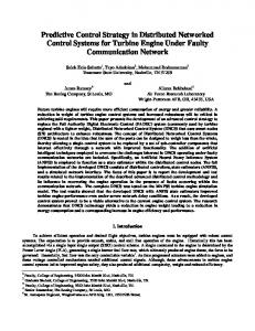
Figure 1.4 The AGC with bilateral contract (Bhowmik et al. 2004).

The system shown in Figure 1.4 consists of three areas with bilateral contracts between the different areas. To guarantee that the frequency is within the limited range the Area Control Error (ACE) and the Generator Control Error (GCE) signals are distributed between the different areas as shown in Figure 1.4. The ACE and the GCE are used to increase or decrease the generated power. Sending these signals through the communication link will introduce time delay and some of these data will be lost. The authors in (Yu et al. 2004)

8

used a simple stability criteria but rather conservative that was reported in the 1980s and introduced in (Mori 1985;Mori et al. 1989). In (Bhowmik et al. 2004) the authors used the simulation to study the effect of the time delay on the load frequency control system. They considered constant and random time delay and studied the effects of the time delay on the stability of the system although they do not give any method to estimate the control system requirements in terms of the maximum time delay. In (Yu et al. 2004) the problem of the load frequency control is formulated as a general time delay problem which is then solved in Linear Matrix Inequality (LMI) form, but it is only applicable to constant time delays. Power electronic systems are among the distributed energy systems that the use of shared network can reduce the complexity in the control interconnections. With the advances in power electronic and the hybrid vehicles these systems will become complex systems and hence the use of the wiring will be complex, expensive, less reliable and bulky. In addition to that a failure in one connection may lead to the failure of the whole system, and hence a suitable communication method is a mandatory. In power electronic system usually many converters are connected in parallel. The main reason for paralleling many converters is to increase the output power while increasing the reliability and reducing the cost and the size of the system. The main issue is to maintain regulated output voltage while achieving a good current sharing. Many control strategies have been proposed and implemented in real applications. These methods can be put under two categories; 1) Communication less methods, 2) Communication based methods. In the communication less method, there is no information transfer between the local converters’ controllers, and the controllers are fully decentralized. These methods cannot guarantee an equal active current sharing between the modules. In the communication based method such as the master-slave control strategy, the modules communicate with each other, and the control tasks

9

are distributed between the local controllers. In large-scale systems, the most complex task is the wiring, and the use of shared network can solve this problem, but the stability of the system must be first analyzed. The most widely used control strategy is the master-slave control strategy which is implemented in (Lai et al. 2009;Mazumder et al. 2005;Mazumder et al. 2008) for a parallel DC/DC buck converter system where a communication network is used to transfer the control signals. Parallel DC/DC buck converter can be found in many applications such as the UPS (Uninterruptible Power Supply) (Shanxu et al. 1999). In parallel DC/DC converters, all the converters should share the load current equally by control connections between the converters. To achieve the active current sharing the reference current signal is broadcast to all the slaves in the system, and hence no direct control connection is required (Lai et al. 2009;Mazumder et al. 2005;Mazumder et al. 2008). The wireless communication is used in an interactive power network in (Acharya et al. 2006) where the authors studied the effects of the network characteristics on the stability and performance of the control system. They proposed that the power network could have three states, which are; nominal, rerouting and clustered state. In the nominal mode, the power modules communicate through the network. When a fault occurs in one of the channels, the signals are rerouted, if the rerouting cannot achieve the stability; then the units enter the clustered mode that implements the decentralized control. In (Zhang et al. 2007) the authors are trying to treat the power electronic modules as communication nodes. The required bandwidth for the different control tasks is estimated, and they are classified into fast, medium-speed and eruptive control loop and depending on these estimations the suitable network is chosen. The authors mentioned that there is a trend towards the integration of both the power electronic and the communication.

10

The Microgrid is one of the possible forms of the power system evolution (Katiraei et al. 2008;Lasseter 2001;Lasseter et al. 2004;Markvart 2006). The Microgrid can be a system of parallel DC/DC converters or parallel DC/AC inverters. In the AC Microgrid in addition to the current sharing requirement the synchronization between the parallel inverters is necessary to eliminate the circulating currents. A good survey on the control techniques and the problem of the communication in parallel three-phase inverters is given in (Mohd et al. 2010;Prodanovic et al. 2000). In the Microgrid there are three different views, two of these views adopt the use of the communication while the other view adopts the decentralized control (Prodanovic et al. 2006). The authors in (Pogaku et al. 2007) claims that the communications based methods can be implemented if the microsources are in close proximity, and the communication link must meet the system bandwidth requirement with a good reliability. With the advances in the network theory and the network technology, the assumption of the small area or close proximity is not required. The communication problem in the Microgrid is discussed in (Green et al. 2007) where the communication link is used for power sharing and synchronization, and the required bandwidth is estimated to be around 100 kbit/s. In the parallel inverters, both the current sharing signal and the synchronization signals are sent through the communication link. Because of the complexity in the wiring, some researchers suggested control strategies without any communication between the converters. All of these methods depend on the so-called droop control method where the active power is used to modulate the voltage and the frequency is modified through the real power (De Brabandere et al. 2004;Ju et al. 2007;Tuladhar et al. 1997). The main drawbacks are the slow dynamic, sharing error, and the method cannot be implemented if the loads are nonlinear. Moreover, since the droop control is a fully decentralized control method it is not superior to the centralized control method because of the slow dynamic

11

and the sharing error. Some researchers suggested the use of low bandwidth communication links to reduce this error, which makes the control system quasi-decentralized. For example, in (Marwali et al. 2004) two control loops are used; one implements the droop control, which is local, and the other loop implements the average power control through a low bandwidth communication link. In the recent years, the Microgrid attracted more attention and the use of shared networks has been considered in many papers. In (Yongqing et al. 2008) a system of two parallel three-phase inverters driving a motor is controlled over CAN (Controlled Area Network) bus where the master-slave control strategy is used to distribute the control tasks between the different inverters. When the distributed energy system implements the quasi-decentralized control strategy over a shared network, it will form a networked control system. From the previous literature, I found that either no method for the stability of the system is given or the authors use some stability analysis methods that are rather complex. In the following section, the basic definitions and issues in NCSs are briefly described.

1.3 Description of Networked Control Systems When a traditional feedback control system is closed via a communication channel, which may be shared with other nodes outside the control system, then the control system is called an NCS (Networked Control System). An NCS can also be defined as a feedback control system wherein the control loops are closed through a real-time network (Wang, F. Y et al. 2008). The defining feature of an NCS is that information (reference input, plant output, control input, etc.) is exchanged using a network among control system components (sensors, controllers, actuators, etc., as shown in Figure 1.5).

12

Plant

Sensor 1

...

Sensor n

Actuator 1

...

Actuator n

Network

Controller Figure 1.5 A Typical Networked Control System

The NCS notation used for the first time by Gregory C. Walsh (Walsh al. 1999). Some researchers refer to NCSs as distributed real-time control systems (Nilsson 1998). Because NCS integrates control systems, communication networks, information theory and computer science, some references refer to NCSs as Integrated Communication and Control Systems ICCSs (Ling et al. 2007) but the NCS notation is used in this thesis. In NCS, the information exchange has various time delays, which are defined as the networked induced delay. This delay may be constant, varied or even random and the time delay modelling is a very challenging research area. This induced delay may degrade the performance of the system or may destabilize the control system. Another point that should be pointed out is the Packet Dropouts which means some data may not have the chance to reach their destination and the question that should be asked here is to what extent can the distributed system survive in the cases of time delay or losing some data? Closing the loop through the shared communication network makes the analysis and design of NCSs complex and the conventional control theory assumptions (such as

13

zero time delay from the sensor to the controller and from the controller to the actuator) became void. Communication networks have been utilized in real-world applications for about thirty years (Baillieul et al. 2007). The main difference between these systems and the networked control systems is that the communication networks were dedicated, while in NCSs they are general-purpose, and the new concepts in communications and networks have been merged with the control concepts, and it became a complete system (single entity) (Wang, F. Y. et al. 2007). NCS is not only a multidisciplinary area closely affiliated with computer networking, communication, signal processing, robotics, information technology, and control theory, but it also puts all these together beautifully to achieve a single system which can efficiently work over a network ( Wang, F. Y. et al. 2008). In addition, NCS has many advantages such as modularity, low costs, reduced weight, decentralization of control, integrated diagnosis, simple installation, quick and easy maintenance, and expandability (it is easy to add/remove sensor, actuator or controller with low cost). NCS can be easily modified or upgraded. NCSs are able to fuse global information to make intelligent decisions over large physical spaces. These points make the NCSs suitable for distributed energy system applications. On the other hand, we have communication constraints, delay, which may be fixed, varied or even random. The absence of a universal clock makes the assumption of constant sampling intervals unrealistic (Ling et al. 2007). Losing some data and the latency of arriving the data due to the network nature makes the system stochastic (Ling et al. 2007).

14

In the classical control theory, the control signals and the sensor signals are pointto-point connected. In the NCS, the situation is quite different because both the actuator and the sensor signals are transmitted through a communication network, and the control system performance will depend strongly on the characteristics of the communication network. The random time delay may cause another problem in the control system which is the packets-out-of-order. The researchers in the last few years concentrated on the following issues: 1- NCS analysis and design. 2- Network architecture, protocols and scheduling. 3- Experimental and simulation studies. 4- NCS modelling (especially time-delay and data dropout modelling). 5- Stability analysis. Non-linear NCS has not been studied extensively (Jiang et al. 2008b). Furthermore, the study of NCSs for a particular application and the use of a specific communication network have not been considered in many papers. The time delay and packet dropouts are characteristics of the network, and even if they can be kept very low with good scheduling and reducing network traffic they cannot be totally eliminated. Therefore, new methods for compensating these two imperfections are very important research areas. There are also other issues such as protocols, scheduling, communication constraints, etc., but these issues affect the time delay and packet dropouts so from control system view point our interest will be in the time delay and data dropouts. In the following section, a brief description of the basic problems concerning NCS is given.

15

1.3.1 Network-Induced Delays in Networked Control Systems: As we discussed previously the network-induced delay may degrade the performance of the system and even may lead to system instability. In the analysis of the NCS, the assumption of constant sampling is not always valid (Ling et al. 2007). Figure 1.6 shows a system with varying time delays.

1

2

3

4

6

5

7

8

Sensor

1

τ1

2

τ2

3

4

6

5

τ3

τ5

τ6

7

τ7

8

τ8

Controller

Figure 1.6 Time Delay in NCS

Time delay can be made small and deterministic by good scheduling and giving some signals high priority, and the system can be treated as an ordinary deterministic time delay system (Nilsson 1998). Time delay affects the performance and the stability. The factors that affect the time delay are: the network load, the network scheduling, the network bandwidth, the message size and the message priority. The time delay in NCSs can be modelled based on the statistics of the time delay. A model that exactly characterizes the network induced delay is difficult to obtain but generally, a good and reliable model can be obtained. Time delay can be dealt with as a constant if the delay introduced by the network is less than the application’s delay (Nilsson 1998).

16

Many researchers proposed control methods to compensate the time delay effects. In (Sadeghzadeh et al. 2008) they solve the time delay problem by using a variable sampling period approach, and a neural network was developed to estimate the time delay. Next, this estimated time delay is taken as the sampling period. However, they restricted their models to time delays less than one sampling period, and they assumed that the time delay is governed by some function. In (Liu et al. 2005) the authors consider random time delay governed by Markov Chains. Some papers proposed fuzzy compensators for the time delays, for example, in (Jiang et al. 2008b) they use T-S fuzzy model for the NCS. Also the model predictive control and the Markovian jump system approach are addressed in many papers. A detailed review on the time delay problem in NCS is presented in Chapter 3.

1.3.2 Packets Dropouts: In some cases due to bandwidth or communication constraints, the message may not be transmitted in a single packet but split into multiple packets. Due to the network nature, these packets may be delayed, or they may be even lost as shown in Figure 1.7 or may arrive but out-of-order as shown in Figure 1.8. Packet dropouts may be considered as a special case of an infinite time delay. 1

3

2

4

6

5

8

7

Sensor 1

2

3

4

5

6

Controller Missing Data

Figure 1.7 Packets Dropouts in NCS

17

7

8

1

3

2

4

5

6

7

8

Sensor 1

2

3

5

4

6

7

8

Controller Out of Order

Figure 1.8 Packets out-of-order in NCS

When a packet is lost there is no need to retransmit it again, an acknowledgement must be sent to transmit a new data. In (Wang, Y.-L et al. 2008) the design of a networked control system based on Lyapunov function is addressed where they took the packet out-of-order into account. In (Millan et al. 2008) the development of a generalized predictive control scheme to overcome the high dropout levels is presented.

1.3.3 NCSs Structures: Networked control system can have one of the following structures (Wang F. Y et al 2008) as shown in Figure 1.9: Direct Structure and Hierarchical Structure. These two structures are found in many distributed energy systems. In the direct structure, the sensors and the actuators are directly connected to the network (and the plant), but the controller is connected to them through the network. Using shared network to transfer the measurements, from sensors to controllers and control signals from controllers to actuators, can greatly reduce the complexity of the connections.

18

Controller

Controller

Network

Sensor

Network

Actuator

Sensor Local Controller

Plant

Actuator Plant

Figure 1.9 (a) Direct Structure of NCS, (b) Hirarchical Structure of NCS

In the hierarchical structure, the system is divided into subsystems; with each subsystem has sensor, actuator and controller in a hierarchical structure. In this structure, the local controllers can communicate with each other and with the central controller to achieve the global goals of the system. This structure can be found in parallel DC/DC and parallel DC/AC converters in Microgrid.

1.3.4 Networked Control System Stability: The stability is a crucial part in designing any control system. In NCS, the main causes of instability are the time delay and the data dropouts. The stability analysis is very complex in the presence of the time delay because the latter introduces an exponential term in the characteristics equation which replaces the algebraic equation with transcendental equation. The control system designer should take the induced time delay and packet dropouts effects into account. An accurate model for the time delay should be obtained in order to incorporate its effect in the control system performance. The time delay depends on many

19

factors such as the network type; the protocol used, the bandwidth and the packet size and as a result the time delay may have one of the following forms; Constant (Fixed) Time Delay, Varied Time Delay and Random Time Delay. In designing NCSs a stability criterion has to be made to ensure system stability under some time delay conditions. The stability theory that has to be applied depends on the network characteristics and hence on the time delay. If the sampling time is equal or larger than the maximum time delay, then the time delay can be treated as a constant time delay and the existing time delay control methodology can be used. The simple stability theories for discrete systems can be applied in this case. In some networks, the time delay may be time varied but periodic and in this case more difficult methods have to be applied. In some cases, the time delay may be random due to the network and protocol characteristics. These random time delays can be modelled based on probabilistic methods, and Markov Chains is one of these methods. The stability analysis of this type of time delay is the most challenging because more advanced and sophisticated techniques must be used to formulate the random delay and nonlinear control theories must be applied. Nilsson (Nilsson 1998) proposed an optimal stochastic control method to control NCSs with random time delay, which is modelled using Markov Chains. Also the Markovian Jump Linear System approach and the model predictive control have been reported in many papers (Liu, Lei-Ming et al. 2005;Liu et al. 2008;Xiao et al. 2000;Yu et al. 2008; Zhang, Guofeng et al. 2008;Wu et al. 2009;Jing et al. 2007). In most of the stability and stabilization control problems, the final stability or controller design is in the form of Linear Matrix Inequality (LMI) which has to be solved numeri-

20

cally. The LMI arises in many control design and stability problems. The applications of LMI in control theory are reported in (Boyd et al. 1995). The LMI has the following form: m

S( x ) = S 0 + ∑ x i S i > 0

(1.2)

i =1

where x ∈ R m is the variable and S i = S Ti > 0 is a positive symmetric constant matrix. The strict LMI in (1.2) is a set of polynomial inequalities in the variable x . The LMI (1.2) is a convex problem that can be solved efficiently using the Matlab toolbox. This form appears in many control problems (Boyd et al. 1995). The advances in convex optimization algorithms made the LMI a powerful design tool. The Matlab developed the LMI toolbox (Gahinet et al. 1995) that implements interior-point algorithms for solving the LMI problems. If the LMI problem can be solved, we say that the LMI is feasible if not it is infeasible. The solution of (1.2) is called the feasible set.

1.4 Main Contributions of the Thesis The contributions of the thesis can be summarized into the following: •

For NCSs with bounded time delays, a new stability and maximum allowable delay bound estimation method has been proposed. The method adopts the finite difference approximation for the delay term in the analysis. A theorem is derived for estimation of the maximum allowed time delay to maintain the system stability. A further derived corollary (Corollary 3.1) has a simple structure in a scalar inequality form for MADB estimation. The results of the estimated MADB obtained through Theorem 3.1 and Corollary 3.1 are comparable with the results obtained through

21

the methods in the previous published literature, however, the method proposed in this thesis has a much simpler procedure in applications. Furthermore, the method links the controller parameters to the MADB and can be used to guide in the process of choosing the controller parameters. The same methodology has been applied to NCS with dynamic controller. Theorem 3.4 and Corollary 3.5 are derived while neglecting the actuator to the controller time delay. While Theorem 3.5 and Corollary 3.6 are derived when the actuator to the controller time delay is not neglected. Theorem 3.7 is proposed for multi-units interconnected system and applied to three generator power system, and the value of the MADB is estimated. It is found that the MADB can be achieved with the current network technology. •

The proposed method has been extended to study the stability and maximum allowable delay bound for a class of nonlinear NCS. A new stability criterion is derived for a class of nonlinear NCS with norm bounded nonlinearity. The theorem is based on writing the norm bounded constraint as LMI and use of the finite difference approximation for the delay term and then the quadratic Lyapunov function is used to derive theorem in LMI form. The results of the theorem have been compared with some of the published results, and the method is simpler while giving comparable results.

•

Due to the component aging, noise in measurements, and slowly time varying parameters all the system performances are subject to uncertainties. A new stability theorem for uncertain NCS with norm bounded uncertainties has been derived. Again, the proposed method is much simpler in applications than those previously published methods.

22

•

When the time delay is governed by Markov Chains the NCS can be modelled as discrete-time Markovian jump system and the stability of the system is formulated as Bilinear Matrix Inequality (BMI). The BMI is not a convex problem and cannot be solved directly. In this thesis, the V-K iteration algorithm is used to solve the BMI where the BMI is divided into three basic LMI problems that can be solved using the Matlab LMI toolbox. The problems to be solved can be considered as three types: feasibility problem, eigenvalue problem and generalized eigenvalue problem. We proposed improved V-K algorithm by maximizing the decay rate in both the V- and K-iteration loops.

•

A parallel DC/DC buck converter system implements master-slave control strategy through a shared network is modelled as NCS, and it is used as one of the case studies. The stability of the system in the presence of the time delay is analyzed. The MADB is estimated, and it is found that the parameters that affect the MADB strongly are the voltage controller gain, the output feedback gain factor, and the load resistance. The stochastic stability of the parallel DC/DC buck converters is analyzed. The range of the voltage controller parameters that achieves the stochastic parameters is determined.

The list of the published papers is given below: [1]

A. F. Khalil and J. Wang, “Time Delay Tolerance Estimation for Linear Control System Stability Analysis using a Finite Difference Method”, In the Proceedings of the 15th International Conference on Automation and Computing, 2009, Luton, UK, pp. 70-75.

[2]

A. F. Khalil and W. Jihong, "A new stability and time-delay tolerance analysis approach for Networked Control Systems," In the Proceeding of the 49th IEEE conference on Control and Decision 2010, pp. 4753-4758.

23

[3] A. F. Khalil and J. Wang, "A New Stability Analysis and Time-Delay Tolerance Estimation Approach for Output Feedback Networked Control Systems," In the Proceeding of the United Kingdom International Control Conference, 2010 pp. 4753-4758. [4] A. F. Khalil and J. Wang, "A New Method for Estimating the Maximum Allowable Delay in Networked Control of bounded nonlinear systems," The 17th International Conference on Automation and Computing (IEEE), Huddersfield, UK 2011, pp. 80-85.

1.5 Thesis Outline The thesis is organised into seven chapters. Chapter 1 is an introductory chapter, and the rest of the thesis chapters are summarized below: Chapter 2 is dedicated to time delay analysis in two control networks which are the CAN and the Ethernet. The time delay modelling is based on the time delay analysis and is crucial part in studying the stability of NCS. We chose the CAN and the Ethernet because they are among the widely used computer networks for control systems. The description of the CAN and the Ethernet with a brief review on the control networks is given in this chapter. The time delay simulation analysis has been carried out using the TrueTime 1.5 simulator whose basic blocks are briefly summarized. A simulation study has been carried out to study the characteristics of the time delay in the CAN and the Ethernet. Different scenarios have been simulated with different message priority, message length, bit rate and network load. Chapter 3 reports the proposed new method for stability analysis and MADB estimation for NCS. The chapter starts with literature review on the time delay problem in NCS. Then the mathematical model for NCS with state feedback controller is represented, and Theorem 3.1 and Corollary 3.1 are derived. Theorem 3.1 and Corollary 3.1 are used to estimate the MADB. Many examples are picked-up from the literature, and the results are compared

24

with those obtained using the proposed method. The same methodology for the NCS with state feedback controller has been applied to NCS with dynamic controller and to multiunits interconnected NCS. For the NCS with dynamic controller, two cases are studied; the first with neglecting the time delay between the controller and the actuator and the second case when the time delay from the controller to the actuator is considered. The results of the theorem and the corollary derived for the multi-units interconnected systems have been applied to a power system consist of three synchronous generators. The MADB for the three generators system is estimated, and the simulation results for the system are carried out to show that the MADB lies within the stability margin. Chapter 4 deals with the stochastic stability of NCS when the time delay is modelled using Markov Chains. At first the jump system is described with a short review on its application in NCS. Then the NCS with both state feedback and dynamic controller are modelled as a Markovian jump system. The sufficient conditions for the stability of the system are given, and the problem is formulated as BMI. The V-K iteration algorithm for solving the BMI is described with the details of solving the three basic problems in the V-K algorithm using the LMI matlab toolbox. The V-K iteration algorithm is applied to the cart and the inverted pendulum problem. Chapter 5 reports the stability analysis and MADB estimation for parallel DC/DC buck converter controlled through a shared network. The model of the parallel DC/DC buck converter is presented in this chapter, and the master-slave control strategy is explained. Then a case study system consists of three parallel DC/DC buck converters is analyzed where the MADB is estimated. The proposed method is compared with one of the published methods. Using the proposed method in chapter 3 the parameters that affect the MADB are studied. Under the bounded time delay assumption, the proposed method for

25

estimating the MADB is used to find the range of the voltage controller gain that gives MADB larger than the worst-case time delay in the CAN and the Ethernet with constant, periodic, and random but bounded time delay. The last section of this chapter is devoted to design a stochastic stabilizing controller for the parallel converters system when the time delay is modelled using Markov Chains. Chapter 6 proposes two new stability and MADB estimation methods, one for a class of NCS with norm bounded nonlinearity and the second method for uncertain NCS. The mathematical model for a class of nonlinear NCS is presented in the chapter, and two stability criteria are derived. The first stability theorem is in LMI form and is based on using the finite difference approximation for the time delay term and writing the nonlinear constraint as LMI. Another stability criterion in scalar inequality form is derived, and the results of the estimated MADB are compared with the results available in the literature. Then the stability of uncertain NCS is studied and a method for estimating the MADB for the uncertain NCS is presented. The stability theorem is in LMI form, and many examples picked from the literature for comparison. Chapter 7 is the concluding chapter where the conclusions drawn from this research are summarized along with some suggested future projects.

1.6 Summary This chapter introduces the thesis from its background, motivation, and main contributions to review of the concepts and current methods. The chapter serves a preparation and overview to the whole thesis.

26

CHAPTER TWO: TIME DELAYS IN SHARED NETWORKS

2.1 Introduction Control networks are the backbone for any networked control system, for instance, a distributed energy system is controlled through a shared network. The induced time delay in a network can degrade the performance of the system or destabilize the system. In networked control systems, the control network is defined as the medium by which the sensors, the actuators and the controllers can exchange their information. The main difference between control networks and data networks is that the control networks can support real-time constraint (the guarantee of receiving the message within a bounded time) which may not be achieved in data networks. Another difference that can designate between these two networks is that both the message length and the bit rate are high in data networks while in control networks, the messages are bursted and short. In this chapter, the time delay is analysed in two candidate control networks, the CAN and the Ethernet. The CAN implements a deterministic protocol where the time delay can be made constant or bounded. On the other hand, the Ethernet is a non deterministic protocol because the network cannot be pri-

27

oritized. In this study TrueTime 1.5 simulator is used. The TrueTime 1.5 simulator operates in Matlab/Simulink environment but m-files for configuring the blocks must be written. A brief description of the simulator is presented in this chapter. The features associated with the time delays in these two networks are studied with different message length, priority, and load. Furthermore, the time delay characteristics are investigated for transmitting either periodic or random messages.

2.2 Time Delays The time delay is defined as the difference between the time of receiving the message and the time of sending the message (Lian et al. 2001). The total time delay, Ttotal , consists of pre processing time delay, T pre , network time delay, Tdn , and post processing time delay,

T post . The pre-processing time delay is composed of analogue to digital conversion, computation time and encoding time. The post processing time delay is composed of digital to analogue conversion, computation time delay and decoding time delay. The network time delay is the time when the data are ready for transmission until the data are received by the designated destination. The network time delay consists mainly of 1) Waiting time delay, T w , the sending node has to wait a specific time until the network becomes idle then it

starts transmission. 2) Retransmission time delay, Tretr , if a collision occurs the sending node should wait for a random time then it starts retransmission. 3) Transmission time delay, Ttr , the time required to transmit the message and it depends on the message length and the bit rate. The time delay is given by: Tdn = Ttr + Tretr + Tw

(2.1)

28

Ttotal = T pre + Tdn + T post

(2.2)

To understand the time delay in computer networks a statistical analysis should be conducted in order to derive the time delay characteristics from their probabilistic distribution. According to (Lian et al. 2001) the parameters that affect the time delay are the access delay, transmission time, response time, message delay, message collisions, message throughput, packet size, network utilization, and determinism boundaries. In this work, we use simple models for the time delay and the network utilization to estimate the time delay and network load. In this case, the time queuing and buffering time delay are represented by the waiting time delay.

2.2.1 Network Schedule Scheduling algorithms are constructed to handle the flow of messages among the network nodes. The performance of the NCS depends strongly on the network scheduling (Branicky et al. 2002). This means to assign a time schedule for all the components in the control systems, which are the sensors, the actuators and the plants. The network scheduling algorithm assigns the message priorities in the network. The NCS can be schedulable if all the tasks within the NCS can be accomplished before the deadline (Branicky et al. 2002).

2.2.2 Network Utilization The network utilization can be defined as the percentage of the total message lengths over the period time or running time, the utilization is given by (Lian et al. 2001):

UT

∑ =

i∈ N node

∑ (T m( i )

j =1

(i , j ) tr

(i , j ) + Tretr )

(2.3)

Tmax

29

(i , j ) where Ttr(i , j ) is the time required to transmit the (i,j)th message from node i to node j. Tretr

is the time required to retransmit the (i,j)th message if a collision has been detected. Tmax is the period of messages transmission. U T is the utilization. m(i ) is the number of the messages to be sent by the ith node. The utilization is used to describe the network load level. Under low load the utilization approaches zero and when the utilization approaches one or larger than one then the network is said to be saturated or overloaded. Different networks can show different time delay characteristics under high utilization load.

2.3 Control Networks Computer networks can be classified into data networks and control networks. Data networks are intended for transmitting data messages such as video, audio, text messages, etc. The Internet and the Ethernet are two of the most well-known examples of data networks. The data networks implement protocols that do not support real time control tasks but intended for transmitting long messages with high bit rate. Although the data networks are characterized by high bit rates and long messages, the receiving of the message within a bounded time slot is not guaranteed. On contrast, control networks implement protocols that support real time constraints and in many cases, the network can be made deterministic. The control networks such as the CAN, Field buses (FIB), and PROFIBUS (Process Field Bus) are found in the industry, and the messages are bursted with relatively slow data rates. Due to the availability of data networks almost in everywhere they gathered a lot of attention to be used as a communication medium for NCS (Montestruque et al. 2004;Chow et

30

al. 2001). One of the candidate networks is the Ethernet that implements the CSMA/CD (carrier-sense multiple access with collision detection) protocol set by the IEEE 802.3 network standard and can support real time constraints.

2.3.1 Controller Area Network (CAN) The motive for developing CAN was from the car industry in order to reduce the cost, weight and complexity in the wiring in a vehicle (Baillieul et al. 2007). The CAN is a serial communication bus developed in 1983 at Robert Bosch GmbH and realized in 1986 (Baillieul et al. 2007). The CAN implements the carrier-sense multiple access protocol with arbitration on message priority (CSMA/AMP) where each node must listen to the network before trying to transmit. The CSMA/AMP is a prioritized deterministic protocol where the nodes or the messages can be assigned to a priority, and the arbitration is used to win the access to the network. The message of the CAN is shown Figure 2.1. The CAN message or frame can be divided into the data frame (broadcast a message to the CAN bus), remote frame (Requests transmission of message), error frame (Signals error condition) and overload frame (Special error frame). The total overhead is 47 bits, and the data message can be from zero to 8 bytes. The identifier in the arbitration field is 11-bit in the standard CAN while it is 29-bit in the extended CAN, which allows 229 priority levels. The abbreviations in Figure 2.1 are: SOF (Start of Frame), RTR (Remote Transmission Request), the DLC (Data Length Code) and the two bits r0 and r1 forms the control field, CRC (Cycling Redundant Code), ACK (Acknowledgement), EOF (End of Frame), int (Interface Space). For more detailed description for the CAN frame the reader can refer to (Bosch 1991).

31

Message Frame Bus idle

Arbitration Field 10-bit identifier SOF

Control

r1 r0

DLC

Data Field CRC Field ACK EOF

Data (0-8) Bytes

int

Bus idle

15 Bits

RTR

Delimiter

Delimiter Slot

Figure 2.1 The message frame format of CAN (Lian et al. 2001) When a node tries to transmit it listens to the network if it is idle, then the node starts to transmit directly. If many nodes are trying to transmit at the same time the arbitration is used to gain access to the network. When two nodes are transmitting at the same time the identifiers are sent if one node receives the same bit it has sent, then that node will win the arbitration. Depending on the bus length the maximum bit rate in the CAN can be up to 1 Mbit/s. The bit rate with different bus lengths is given in Table 2.1. The number of the nodes in the CAN depends on the network utilization and for a higher number of nodes; the multilevel network approach can be used. However, the CAN is a deterministic protocol that guarantees a fixed time delay for the highest priority node; the bit rate is low compared to other networks such as the Ethernet.

Table 2.1 The bit rate with different bus lengths (Corrigan 2008) Bus Length/ m Bit Rate Mbit/s

25 1

50 0.8

100 0.5

250 0.25

500 0.125

1000 0.05

2500 0.02

5000 0.01

2.3.2 Ethernet The Ethernet is one of the most widely used local area networks (LANs). The Ethernet is mainly intended for transmitting large data messages and was introduced in beginning of the 1980s. In contrast to the CAN, the Ethernet is not a deterministic protocol because it

32

implements the carrier-sense multiple access with collision detection (CSMA/CD). The bit rate in the Ethernet can be ranged from the standard 10 Mbit/s up to 100 Gbit/s. The Ethernet message is shown in Figure 2.2. The Preamble bits for synchronization and the start of delimiter are 8 bytes, and the minimum message length is 64 bytes.

Bytes 7

1

Preamble

Start of Delimiter

6 Destination Address

6 Source Address

2 Data Length

Overhead = 22 Bytes

0-1500 0-46 Data

Pad

4 Checksum

46-1500 Bytes OH=4 Bytes

Figure 2.2 The message frame format of Ethernet (Lian et al. 2001) The minimum packet size in the Ethernet is 46 bytes and if the data message is less than 46 bytes padded bits are automatically added to make the data message 46 bytes. Including the overhead and checksums bits, the minimum Ethernet message is 72 bytes. When any node starts to initiate a transmission, it listens to the network if a collision is detected the node waits for a random time specified by the binary exponential back of algorithm (BEF) (Lian et al. 2001). This random time is randomly chosen between zero and (2n-1) slot time (Ethernet message transmission time), where n is the number of collisions detected by the node. For a 10 Mbit/s Ethernet the slot time is 51.2 µs (=512/10,000,000). After ten collisions the retransmission time is fixed to 1023 slot time (Lian et al. 2001). As the number of the collisions exceeds sixteen, the network reports transmission error to the sending node. The main disadvantage in the Ethernet is the unfairness in the Ethernet protocol. Under heavy load the number of collisions will be high, and the protocol cannot guarantee an equal chance to all the nodes, and the time delay in this case may not be bounded which violates one of the networked control system requirements.

33

2.4 TrueTime 1.5 Simulator TrueTime 1.5 is a software based on Matlab/Simulink, and it is dedicated to the simulation of real-time control systems (Andersson et al. 2005;Henriksson et al. 2004;Henriksson et al. 2006;Sui et al. 2010). The software is based on Matlab/Simulink but source code programs in Matlab or C++ (needs a compiler) must be written to initialize the TrueTime blocks and to be executed during the run. TrueTime 1.5 simulator is freeware developed in Lund University and can be downloaded free from http://www.control.lth.se/truetime. The TrueTime Library is shown in Figure 2.3. The TrueTime 1.5 simulator contains six basic blocks, which are the kernel, the network, the wireless network, the battery, the sending and the receiving blocks.

Figure 2.3 The TrueTime Block Library.

The TrueTime 1.5 simulator blocks are connected with the ordinary Simulink blocks to form a real-time control system such as the networked control system. Before a simulation can be run, however, it is necessary to initialize kernel blocks and network blocks, and to create tasks, interrupt handlers, timers, events, monitors, etc., for the simulation. The TrueTime 1.5 supports networked control system simulation. In the following section, the time delay is studied in the CAN and the Ethernet using the TrueTime 1.5 simulator.

34

2.5 Simulation Results for the CAN and the Ethernet Different scenarios have been implemented in the TrueTime 1.5 simulator to study the time delay in two popular control networks, which are the Ethernet and the CAN. The simulator supports only packet level simulation so the parameters that will be considered are the bit rate, the message size, the priority and the utilization.

2.5.1 The Time Delay Analysis in the CAN The CAN is a deterministic protocol intended for short messages. In this simulation study, the CAN has seven nodes that represent the load and the system nodes. Three nodes represent the system while the other four simulate the load on the network. The parameters that affect the time delay are investigated; these are the priority, the bit rate, the message length, the utilization, and the message type (periodic messages or random messages). The TrueTime 1.5 Simulink implementation of the CAN with seven nodes is shown in Figure 2.4. The system node has middle priority on the network, but the system nodes are the only active nodes in the network. The system nodes are actuator1, actuator2 and the sensor. This simulates a distributed energy system implementing the master-slave control strategy. The following cases are considered: •

Under no Load: The system nodes are the only active nodes in the network.

•

Periodic Load: All the nodes in the network are periodic.

•

Random Load: The load nodes are random.

35

Network

Node 1 (Interference ) [clock]

[Snd 1]

snd1

rcv 1

From 13

[Rcv1]

[Rcv1]

Goto 12

From 14

Goto 10

Goto 11

snd3

Rcv Snd

From 4

[Rcv3]

Scope 1

Goto 5 Node 1 (Interference )2

Goto 2

Snd1

Clock

[Snd 2]

S

Sensor

To Workspace1

From 2 rcv 4

[Snd 4] From 1

[Rcv3]

[Rcv4]

rcv 5

Rcv Snd

From 5

Goto 3

snd4

[Snd 3]

[Rcv2]

Node 2

Goto 6

Td

Node 1 (Interference )3

[Rcv6]

Rcv

From 12 Goto 1 [Snd 2]

[Rcv4]

Rcv Snd

D/A1

[clock] rcv 6

From 6

[Rcv6]

Goto 7

Scope 12 Scope 3

Actuator 1

snd6

R1 To Workspace4

Node 2 (Actuator )1

[Rcv7] Goto 9

[clock] From 11

snd7

Rcv 1

From 8

Goto 4

rcv 7

To Workspace2

[Snd 4]

snd5

From 10

Goto 8

Snd A/D1

[Rcv2] rcv 3

[Snd 5]

Node 1

snd2

From 3

[Snd 3]

[Snd 1]


rcv 2

[Snd 5]

Rcv Snd

T To Workspace

rcv 8

Td 1 [Rcv7]

Rcv

To Workspace 3

From 7 Scheduling

D/A1

[clock]

Rcv 1

From 9

Actuator 2

Scope 2 Scope 4 R2 To Workspace5

Figure 2.4 The CAN with seven nodes

1) Under no load condition: The sampling period for the system node is 0.01 s and only the system node is active on the network. The time delay with four byte and eight byte messages is shown in Figure 2.5. The bit rate is 100 Kbit/s and the total message length is 94 bits for the four bytes message and 128 bits for the eight byte message. As can be seen from Figure 2.5 the time delay is almost constant under low load condition. With four byte message, the time delay consists of the transmission time which is 0.94 ms in addition to 0.1 ms analogue to digital conversion time delay and actuator time delay, then the total time delay is 1.04 ms. With eight byte message the total time delay is 1.38 ms because the waiting time delay, and the retransmission time delay are also zero.

36

-3

1.6

x 10

1.4

Time Delay (sec)

1.2 1 0.8 0.6 0.4 0.2 0

0.5

1

1.5

2

2.5

3

3.5

4

4.5

5

Time (sec)

Figure 2.5 The time delay in the CAN with low load, solid-line 94 bit message, dashedline 128 bit message.

The network schedule in Figure 2.6 shows that the system node is the only active node in the network, and it has the second priority in the network. Since only the system node is active then the utilization with 128 bits message is given by:

UT =

128 / 100,000 = 0.0128 0.01

This shows very low network utilization. Two different simulations with the system node has a high and low priority, and we observed no change to the time delay characteristics, and it is almost constant.

37

Network Schedule

7

Actuator 2

6

Actuator 1

5

Interference 4

4

Interference 3

3

Interference 2

2

Sensor

1

Interference 1 0

0.01

0.02

0.03

0.04

0.05

0.06

0.07

0.08

0.09

0.1

Time (sec)

Figure 2.6 The Network Schedule

2) The Load is Periodic: In the second scenario, all the activities on the network are periodic. The system nodes use 5 ms period for the transmission while the period of the load messages is 0.1 s. As expected the time delay will be periodic because all the activities on the network are periodic, and the CAN implements a deterministic protocol. The time delay is shown in Figure 2.7. From Figure 2.7 the time delay is periodic with 0.1 s period. The time delay has three different values, which are 1.48 ms, 1.58 ms and 5.2 ms. The time delay behaviour can be explained by looking at the scheduling in Figure 2.8.

38

-3

6

x 10

Time Delay (seconds)

5

4

3

2

1

0

0

0.1

0.2

0.3

0.4 0.5 0.6 Time (seconds)

0.7

0.8

0.9

1

Figure 2.7 The time delay with periodic load messages

Since the system node has a middle priority on the network, there are mainly three possible states for the network. The first state is when the system node starts to transmit, the network is idle and so the time delay will only have transmission time delay component which is 1.48 ms (in addition to the pre, and post processing time delay). The second state occurs as the system node starts to broadcast, the lower-priority node that has already occupied the network and hence the system node will wait until that node finishes the transmission. Then it starts to transmit and in this case we will have a small waiting time delay component in addition to the transmission time delay, and the total time delay in this case is 1.58 ms.

39

5.5

Interference 4

5

Network Schedule

4.5

Interference 3

4 3.5

Interference 2

3 2.5

Sensor

2 1.5 1

Interference 1 0

0.05

0.1 0.15 Time (seconds)

0.2

0.25

Figure 2.8 The network schedule with periodic messages load.

The sensor scheduling signal has three different values, which are low, medium and high. When the signal is low, the sensor node is idle and when it is medium then the sensor node is waiting for the network to become idle. The signal becomes high when it is already occupied the network. The last state has a time delay of 5.2 ms, in this case the system node will wait for the higher-priority node to finish its activity in the network, and the system node should wait until the network becomes idle, the total time delay is then:

Td = Ttr + Tretr + Tw = Ttr + 0 + Tw =

3 ⋅ 128 128 +0+ = 5.1ms 100,000 100,000

In addition to 0.1 ms pre- and post-processing time delay, the total time delay is 5.2 ms as shown in Figure 2.8. The network utilization is given by:

40

UT

∑ = =

∑ (T m (i)

i ∈ N node

j =1

(i, j ) tr

(i , j ) ) + Tretr

Tmax

3 ⋅ 128 / 100,000 128 / 100,000 3 ⋅ 128 / 100,000 + + = 0.3328 0.1 0.005 0.1

The network utilization is still medium. With different priorities, we noticed that with increasing the load with periodic messages the time delay is periodic with different periodic forms even with high utilization. As the network utilization is less than one then the receiving of the message is guaranteed, and this is the advantage of the deterministic protocol.

3) The Load is Random When all the messages are random, the time delay is expected to be random even with deterministic network. In this scenario, we have a CAN with seven nodes; three are assigned as the system nodes and four as the load nodes which are random. In (Nilsson 1998) the message length is chosen to have a uniform distribution but in our case, the activities of the four nodes are random with constant message length, which simulates the non periodic activity on the network. The bit rate is 500 kbit/s and the message’s length is 94 bits. The load messages have 0.01 s period while the system node has 5 ms period. The time delay when the system node has a middle priority is shown in Figure 2.9. The time delay has three different states, which are 0.1 ms, 5 ms and 9.8 ms. The histogram of the time delay in Figure 2.9 is shown in Figure 2.10. The time delay has three states that can be modelled using Markov Chain. The network schedule is shown in Figure 2.11. In many simulations with different message lengths and priorities, the time delay is random with different distribution functions due to the random messages in the network.

41

0.012

0.008

0.006

0.004

0.002

0

0

0.02

0.04

0.06

0.08 0.1 0.12 Time (seconds)

0.14

0.16

0.18

0.2

Figure 2.9 The time delay with random messages and middle priority

500 450 400

Number of Samples


0.01

350 300 250 200 150 100 50 0

0

0.002

0.004

0.006

0.008

0.01

0.012

0.014

Time Delay, sec

Figure 2.10 The histogram of the time delay in Figure 2.9

42

0.016

2.8 2.6

Network Schedule

2.4 2.2

Sensor

2 1.8 1.6 1.4 1.2 1

Interference 1 0

0.02

0.04

0.06

0.08 0.1 0.12 Time (seconds)

0.14

0.16

0.18

0.2

Figure 2.11 The network schedule with random messages load.

From the network schedule in Figure 2.11 we noticed in many cases when the sensor node starts to transmit the network is idle, and the time delay will only have transmission time delay component. The idle network can represent the low state in Markov chain. Another interesting property is that when the current state is the low state then the next state will be either the high state or the low state as can be seen from Figure 2.9. In the medium state when the sensor node starts to transmit the higher priority is already occupied the network. The time delay when the load message has a period of 0.012 s is shown in Figure 2.12, and the distribution function is shown in Figure 2.13. We found that in some cases the time delay can be modelled using Markov Chains.

43

0.02 0.018


0.016 0.014 0.012 0.01 0.008 0.006 0.004 0.002 0

0

1

2

3

4 5 6 Time (seconds)

7

8

9

10

Figure 2.12 The time delay with random messages and middle priority and 0.012 s load message 1400

1200

Number of Samples

1000

800

600

400

200

0

0

0.002

0.004

0.006 0.008 0.01 Time Delay, seconds

0.012

0.014

0.016


44

From the distribution in Figure 2.13 it can be seen that the time delays are mostly distributed around 1 ms with some time delays are uniformly distributed in the interval [2 ms, 9 ms]. The average time delay is 2.5 ms and the maximum time delay is 9.8 ms, this can be explained by looking at the scheduling in Figure 2.14.

3 2.8 2.6

Network Schedule

2.4 2.2

Sensor

2 1.8 1.6 1.4 1.2 1 0.4

Interference 1 0.42

0.44

0.46

0.48 0.5 0.52 Time (seconds)

0.54

0.56

0.58

0.6

Figure 2.14 The network schedule with random messages load.

In most of the time, the network is idle and there is no waiting time delay and hence the time delay will have only transmission time delay, which is 1.04 ms and this explains the large distribution around 1 ms. The load message is a random signal with 9.5 ms width. In some cases when the sensor node is trying to transmit, the load message is already occupied the network which causes the time delay to be distributed between 2 ms and 9 ms. The time delay and the distribution function when the load message has 0.009 s period are shown in Figure 2.15 and Figure 2.16.

45

0.1 0.09


0.08 0.07 0.06 0.05 0.04 0.03 0.02 0.01 0

0

1

2

3

4 5 6 Time (seconds)

7

8

9

10

Figure 2.15 The time delay with random messages and middle priority with 0.009 s load message

1400

1200

Number of Samples

1000

800

600

400

200

0

0

0.02

0.04

0.06 0.08 Time Delay, seconds

0.1

0.12

0.14


46

From the distribution in Figure 2.16 the time delay distribution has a Dirac shape with 9.8 ms average values. The network scheduling is shown in Figure 2.17.

2.8 2.6

Network Schedule

2.4 2.2

Sensor

2 1.8 1.6 1.4 1.2 1

Interference 1 0

0.1

0.2

0.3 Time (seconds)

0.4

0.5

0.6

Figure 2.17 The network schedule with random messages load. It can be seen from Figure 2.17 that the load occupies the network most of the time which increases the time delay. With different priorities we found that the priority affects the average time delay. Increasing the priority reduces the average time delay.

2.5.2 The Time Delay Analysis in the Ethernet The Ethernet is a non deterministic protocol and even with periodic messages on the network the time delay is not expected to show any periodicity. The simulated Ethernet consists of seventeen nodes three of which are the system nodes while the other fourteen nodes are assigned as the load nodes. The TrueTime 1.5 Simulink implementation of the network is shown in Figure 2.18.

47

Node 12

Node 1 Network [Snd 1]

[Snd 2]

[Rcv1]

snd1

From 13

rcv 1

Rcv Snd

[Rcv1]

[Snd 1]

[Rcv12 ]

Node 13

snd2 rcv 2

From 10 [Snd 3]

rcv 3

From 2 [Snd 4]

Goto 21

snd3

snd4 rcv 4

[Rcv3] Goto 2

[Rcv2]

[Rcv2]

Rcv Snd

Goto 1

[Rcv4]

[Snd 2]

snd5

rcv 5

snd6

rcv 6

From 3 [Snd 6] From 8 [Snd 7]

snd7

From 9 [Snd 8]

rcv 7 rcv 8

[Rcv5] Goto 12

[Rcv3]

Rcv Snd

[Rcv7]

Goto 3

[Rcv6]

Node 14 [Snd 3]

[Rcv14 ]

[Rcv4]

Rcv Snd

[Snd 4] (Sensor )

Node 5 [Rcv5]

Rcv Snd

[Snd 10 ]

[Rcv8]

rcv 10

Goto 10

Scope 7

snd10 rcv 11

[Rcv10 ]

[Rcv9]

Node 6 [Rcv6]

Rcv Snd

Goto 13

[Snd 6]

Clock

snd11

rcv 12

snd12

rcv 13

Goto 14

From 17 [Snd 12 ] From 18 [ Snd 13 ]

snd13

From 19 [Snd 14 ]

rcv 14 rcv 15

[Rcv12 ] Goto 16

[Rcv14 ]

Node 7 (Actuator -1)

[Rcv11]

[Rcv7]

Rcv Snd

From 20 [ Snd 15 ]

[Snd 7] [Rcv16 ]

Goto 15 Node 8 [Rcv13 ]

[Rcv8]

Rcv Snd

Rcv

From 12

D/A1

[Snd 8] Clock1

Node 9

Scope 3

Goto 20 [Rcv9]

Rcv Snd

[Snd 9]

snd15

(Actuator -2) rcv 17

From 21 snd16

rcv 18 snd17

Scope 12

Rcv 1

Goto 19

snd14 rcv 16

Scope 1

To Workspace

From 16 [Snd 11]

Goto 8

A/D1

[Snd 5]

T

snd9

From 15

[Snd 15 ]

Snd Snd1

rcv 9

[Snd 9]

[Snd 14 ]

Rcv Snd

snd8

From 11

[Snd 13 ]

Rcv Snd

Node 4

Goto 4

Goto 9

[Rcv13 ]

Node 3

From 1 [Snd 5]

[Snd 12 ]

Rcv Snd

Node 2

[Rcv16 ] Goto 22

Node 10 [Rcv17 ] [Rcv17 ]

[Rcv10 ]

Rcv Snd

[Snd 10 ]

Rcv

From 7

D/A1

Goto 23 Node 11 [Rcv11]

Rcv Snd

Scope 4

Rcv 1

[Snd 11]

Clock2 Scope 2

Figure 2.18 The Ethernet with seventeen nodes The bit rate is the standard 10 Mbits/s bit rate, and the system message length is 576 bits with 5 ms period. All the load messages are periodic with different message lengths. The time delay under low load is shown in Figure 2.19. The periods of the messages are 5 ms, which makes the utilization 0.1728. The network schedule is shown in Figure 2.20, which shows that the system node has assigned the number fifteen because the Ethernet does not support any prioritization. Since the protocol is nondeterministic we can see that under low load, there are no collisions in the network and hence the time delay is constant and can be calculated as:

Tdn = Ttr + Tretr + Tw = Ttr + 0 + Tw =

567 + 0 + 0 = 5.67 ⋅ 10 −5 10,000,000

Ttotal = T pre + Tdn + T post = 0.00001+ 5.67 ⋅ 10−5 + 0.0001 = 1.676 ⋅10−4 sec

48

-4

1.8

x 10

1.6

Time Delay (sec)

1.4 1.2 1 0.8 0.6 0.4 0.2 0 0

0.5

1

1.5

2

2.5

3

3.5

4

4.5

5

Time (sec)

Figure 2.19 The time delay in the Ethernet with low load

18 16

Network Schedule

14 12 10 8 6 4 2 0

0

0.005

0.01

0.015

0.02

0.025

0.03

0.035

0.04

0.045

0.05

Time (sec)

Figure 2.20 The network schedule in the Ethernet with low load

49

When the load messages have a period of 2 ms, the utilization is 0.4147 s. At this utilization level the time delay and the histogram are shown in Figure 2.21 and Figure 2.22. When the network is loaded, we can see that there is a considerable time delay because many messages are trying to transmit at the same time. Both the time delay and the histogram proves that the time delay is random but bounded and in this case, we have not observed any correlation between the previous, current and next time delay.

-3

2.5

x 10


2

1.5

1

0.5

0

0

0.5

1

1.5

2 2.5 3 Time (seconds)

3.5

4

4.5

Figure 2.21 The time delay in the Ethernet with medium load

50

5

800 700

Number of Samples

600 500 400 300 200 100 0

0

0.5

1

1.5 2 2.5 Time Delay, seconds

3

3.5

4 -3

x 10


The main disadvantage in the Ethernet appears when the network is nearly loaded. With 1 ms load period the utilization is 0.8179 and the time delay is shown in Figure 2.23. In this case, the time delay may not be bounded because the network is loaded. Due to the large number of collisions at this utilization level the retransmission time is increasing dramatically, and the Ethernet protocol cannot guarantee a fair bandwidth distribution between the nodes. When a collision occurs in the Ethernet, the node waits for a random time after ten collisions the waiting time is fixed and after sixteen collisions, a transmission error is sent back to the sending node. The main disadvantage for this protocol is that it cannot guarantee receiving the messages within a bounded time.

51

0.4 0.35

Time Delay (sec)

0.3 0.25 0.2 0.15 0.1 0.05 0

0

0.5

1

1.5

2

2.5

3

3.5

4

4.5

5

Time (sec)

Figure 2.23 The time delay in the Ethernet with medium utilization

2.6 Discussions In both the Ethernet and the CAN under very low load conditions, the time delay is almost constant and depends only on the message length and the network bit rate. With prioritized network even when a node has a low priority the time delay is constant under low network utilization levels. When all the activities on the network are periodic, the time delay will also be periodic in a deterministic network. The node priority does not affect the characteristics of the time delay but when the network is overloaded the node with the higher priority will have a guaranteed transmission while the transmission of the lower-priority nodes will not be guaranteed. In the CAN with random messages the time delay is random, and in some cases it can be governed by Markov Chain when the network utilization is low or medium. When the messages are random in the CAN, the time delay can show different

52

probability distribution functions. Increasing the utilization increases the average time delay, and reducing the priority increases the average time delay. Although the Ethernet protocol is not a deterministic protocol, the time delay is constant with periodic messages under very low load condition. Under the condition of low network utilization the time delay becomes periodic even though the protocol is random because the number of collisions is still very low. At the medium and high utilization the time delay is random. When the network is nearly overloaded, the transmission is not guaranteed. From the previous discussion, the following can be concluded: •

The time delay has five different patterns: Constant, Periodic, Random but bounded, Random governed by Markov Chains and random but unbounded. The constant time delay model can be used if the maximum time delay of the system is much larger than the worst-case time delay.

•

The time delay can be affected by the bit rate, message length, priority and utilization.

Depending on the time delay analysis in this chapter two proposed methods will be introduced in the next chapters. In the first method, the time delay is assumed to be bounded and this is the case when the time delay is constant, periodic or random. The worst-case time delay is used to model the time delay under the assumption that the time delay is constant, and this can be achieved through using a buffer. On the other hand, when the time delay is random and governed by Markov Chain the discrete time Markovian jump system approach is used to study the stochastic stability of the system.

53

2.7 Summary In this chapter, a brief introduction to control networks was given. Mainly, two candidates of control networks are discussed; they are the CAN, which is a deterministic network, and the Ethernet, which is a non deterministic network. As the Ethernet was originally intended for data transmission, it is characterized by long data message and high bit rate compared to the CAN. Control networks are the backbone for all the networked control systems and in order to design a networked control system the time delay induced with these networks needs to be pre-analyzed. To characterize the time delay TrueTime 1.5 Simulator is used, which is intended for real time control systems simulation. Different scenarios have been simulated, and it is found that the time delay can be constant, periodic and bounded, random and bounded, random governed by Markov Chain and in some cases, the time delay can be random and unbounded. The main difference between the CAN and the Ethernet appears under high utilization where the time delay can be unbounded in the Ethernet. Depending on these models for the time delay, two analysis methods for NCSs have been proposed in this thesis. The first method is introduced in Chapter 3 and is based on the assumption that the time delay is either constant or bounded. The second method in Chapter 4 can be used whenever the time delay is random and governed by Markov chain.

54

CHAPTER 3: MAXIMUM ALLOWABLE DELAY ESTIMATION FOR NETWORKED CONTROL SYSTEMS

3.1 Introduction Time delays may degrade the performance of NCSs or may lead to system instability. There are many methods reported in the literature for analyzing the stability of time delay systems. However, most of them are very complex to use in practice. Therefore, there is a need for a simple and easy method in terms of engineering design and using by practical engineers. From the analysis in Chapter 2 the time delay can be constant, periodic, or random but bounded. This chapter presents a new method for analyzing the stability of NCSs that can be used as a guideline tool for designing the controller. The detailed description of the proposed method for estimating the maximum time delay in NCSs is presented in this chapter. At first, the method is applied to a single-unit NCS with a state feedback controller (Khalil et al. 2010a). A few examples are illustrated, and the results are compared with that proposed in the previously published literature. The method is then extended to an NCS with a dynamic controller (Khalil et al. 2010b) with an application to a multi-units

55

distributed interconnected NCS, which are used in many distributed energy system application cases such as electrical power systems, parallel DC/DC converters, parallel DC/AC inverters, and Microgrids. A small-scale power system consisting of three generators is studied as a demonstration example and the MADB for the system is estimated using the proposed method.

3.2 Time delays in networked control systems A typical organization of an NCS is shown in Figure 3.1. As the control loop is closed through a communication network, the time delay and data dropout are unavoidable. This may degrade the performance of the NCS or even destabilize the system. In general, the control systems with time delays can be classified into time delay independent (where the stability is not affected by the time delay) and time delay dependent (where the time delay does affect the stability) (Mahmoud 2000). Time delay, no doubt, increases complexity in the process of analysis and design of NCSs. Conventional control theories built on a number of standing assumptions, including synchronized control and non delayed sensing and actuation must be re-evaluated before they can be applied for NCSs (Mahmoud et al. 2003). Analytical and graphical methods have been studied in (Marshall et al. 1992). The stability criteria for NCSs based on Lyapunov-Krasovskii functional approach has been reported in (Tang et al. 2008;Yue et al. 2004a;Yue et al. 2004b;Liu 2003).

56

Controller

Sensor 1

Sensor 2 Local Controller 2

`

Plant 4

Plant 2 `

Supervisor Controller

Local Controller 1

`

Plant 3

Plant 1

Figure 3.1 A Typical Networked Control System

The main goal of the most-recent work in this field is to reduce the conservativeness of the stability region by using Lyapunov-Krasovskii functional approach with improved algorithms for solving the Linear Matrix Inequality (LMI) set although, at expense of increased complexity and computation time. In (Yue et al. 2004a;Yue et al 2004b), a LyapunovKrasovskii function is used to derive a set of LMIs and the stability problem is then formalized as a feasibility LMI problem. In many of the previously reported works, the controller is designed in the absence of the time delay. In (Jian et al. 2008), an improved Lyapunov-Krasovskii function is used with triple integral terms. The LMI methods require that the closed-loop system to be Hurwitz (De Souza et al. 1995;Liu 2003;Zhang et al. 2001). In (Wu et al. 2007), a modified Cone Complementary linearization algorithm based on the Lyapunov-Krasovskii approach is implemented. The method reported in (Zhu et al. 2008) is claimed to be less conservative, and the computational complexity is reduced. An LMI method in the frequency domain is derived in (Jun et al. 2000), which is then transformed on to an equivalent non-frequency domain LMI by applying Kalman-YakubovichPopov Lemma. It has been reported that the ordinary Lyapunov stability analysis is linked

57

by a suggested variable to state vectors through convolution (Kim 2005), and the stability analysis is simplified to only require solving a nonlinear algebraic matrix equation. In (Zhang et al. 2001), the hybrid system technique is used to derive a stability region, and an upper bound is derived for the time delay in an inequality form. Comparing with the other published results, the results are rather conservative. The hybrid system stability analysis technique has also been used in (Branicky et al. 2000). A simple analytical relation is derived between the sampling period, the time delay and the controller gains. The same approach is used in (Xei et al. 2002) with more conservative stability region results. The model-based approach for deriving necessary and sufficient conditions for the stability is presented in (Montestruque et al. 2004). The stability criteria are derived in terms of the update time and the parameters of the model. The model-based approach is then extended to study the stability of a distributed interconnected NCS in (Sun et al. 2008). The optimal stochastic control was studied in (Nilsson 1998) with a discrete time system model where the random time delays are modelled using Markov Chains, and the controller uses the knowledge of the past state time delays by involving time stamping. Most of the previously developed approaches require excessive load of computations, and also for higher-order systems; the load of computations will increase dramatically. In practice, engineers may find it difficult to apply those available methods in control systems design because of the complexity of the methods and lack of a guideline in linking the design parameters to the system performance. Almost all the design procedures highly depend on the post-design simulation to determine the design parameters. So there is a demand for a simple design approach with clear guidance for practical applications. In this chapter, a new stability analysis and controller design method is proposed, in which the design approach is simpler and a clearer design procedure is given.

58

3.3 Maximum allowable delay bound estimation for NCSs Although the issues involved with time delays in control systems have been studied for a long time, it is difficult to find a method simple enough to be accepted by control system design engineers in industry. It is found that the most previously reported methods rely on LMI techniques, and they are generally too complicated for practical engineers to use and also involve heavy load of numerical calculations and computation time. A new method is proposed in this chapter, which has a simple structure and is used for estimating the maximum time delay allowed while the system stability can still be maintained. In control systems, the sampling time is preferred to be small (Park et al. 2002). The Maximum Allowable Delay Bound (MADB) (Yang et al. 2007;Khalil et al. 2010a;Khalil et al. 2010b;Khalil et al. 2011;Kim et al. 2003;Cheng et al. 2007) can be defined as the maximum time delay presented to the system while the system stability is retained if without considering the system performance.

3.3.1 The mathematical model of a single unit NCS A continuous-time invariant linear system is given by:

x& (t ) = Ax(t ) + Bu(t )

(3.1)

y (t ) = Cx(t ) + Du(t ) where x(t ) ∈ ℜ n is the system state vector, u(t ) ∈ ℜ m

is the system control input and

y (t ) ∈ ℜ p is the system output. A ∈ ℜn×n , B ∈ ℜ n× m , C ∈ ℜ p× n and D ∈ ℜ p× m are constant matrices with appropriate dimensions.

59

Suppose that the control signals are connected to the control plant through a kind of network, so the time delay is inevitable to be involved in the feedback loop as shown in Figure 3.2. The state feedback can therefore be written as: u(t ) = Kx (t − τ )

(3.2)

Actuator

Plant

Sensor

x(t )

τ

Kx(t − τ )

Controller

x(t − τ )

Figure 3.2 An NCS with time delay between the sensor and the controller

where τ is the equivalent time delay and K represents the feedback control gains with appropriate size. The time delay may be constant, variable or even random. In NCSs, the time delay is composed of delays from sensors to controllers, in controller and controllers to actuators, which can be expressed by:

τ = τ sc + τ c + τ ca

(3.3)

where τ sc is the time delay between the sensor and the controller, τ c is the time delay in the controller, τ ca is the time delay from the controller to the actuator. For a general formulation, the packet dropouts can be incorporated into (3.3):

τ = τ sc + τ c + τ ca + dh

(3.4)

60

where d is the number of dropouts and h is the sampling period. In (3.4) the data dropouts can be considered as a special case of time delay (Zhang et al. 2008a;Zhang et al. 2008b). It is supposed that the following hypotheses hold.

Hypothesis 3.1 (H 3.1): i.

Sensors are clock driven.

ii.

The controllers and the actuators are event driven.

iii.

The data are transmitted as a single packet.

iv.

The old packets are discarded.

v.

The matrix (I n×n + τBK ) −1 is non-singular.

vi.

All the states are available for the measurement and hence for the transmission.

Hypothesis 3.2 (H 3.2): The time delay τ is small enough for the finite difference approximation to be held. Definition 1 (D1): For a function f (t ) , the nth order reminder for its Taylor’s series expansion is defined by (Meyer 2000) ∞

Rn ( f ( x), τ ) = ∑ n

f

(n)

(x) n τ n!

3.3.2 Maximum allowable delay bound estimation in the time domain Applying the state feedback proposed in (3.2) to the system (3.1), we have: x& (t ) = Αx(t ) + BKx (t − τ )

(3.5)

Equation (3.5) can be rearranged as:

61

x& (t ) = ( A + BK)x (t ) + BK [ x(t − τ ) − x(t )]

(3.6)

Theorem 3.1: Suppose that H 3.1 and H 3.2 hold. For System (3.1) with the feedback control of (3.2), the closed-loop system is globally asymptotically stable if λi (Ψ) ∈ C − for i = 1, 2, L , n and all the state variables’ 2nd order reminders are small enough for the given value of τ, where Ψ is given by: Ψ = [(I n×n + τBK ) −1 ( A + BK )]

(3.7)

Proof: The expression for x(t − τ ) can be obtained by Taylor Expansion as (Meyer 2000): ∞

x(t − τ ) = ∑ (−1) n n =0

τn n!

x ( n ) (t )

(3.8)

or x(t − τ ) = x(t ) − τx& (t ) + R 2 (x, τ )

(3.9)

From (3.9) it can be seen that R 2 (x,τ ) depends on the time delay, τ , and the higher-order derivatives of x(t ) . If τ is small enough, all the elements of R 2 ( x,τ ) are small enough to be ignored. Then we have: x(t − τ ) − x(t ) ≅ −τx& (t )

(3.10)

Substituting (3.10) into (3.6), the following can be derived: x& (t ) ≈ ( A + BK)x (t ) − τBK x& (t )

(3.11)

(I + τBK ) x& (t ) ≈ ( A + BK)x (t )

62

x& (t ) ≈ [(I + τBK ) −1 ( A + BK)]x(t )

(3.12)

Ψ = [(I + τBK ) −1 ( A + BK )]

(3.13)

Therefore, the system (3.12) will be globally asymptotically stable if

λi (Ψ) ∈ C − for i = 1, 2, L , n

□

Corollary 3.1: Suppose H 3.1 and H 3.2 hold. For the control system (3.1) with the control law (3.2), the closed-loop system is globally asymptotically stable if

τ
0

∀ x≠0

(3.15)

& ( x) < 0 , ∀ x ≠ 0 The objective for the next step is to find the range of τ that will ensure V

(Goodall et al. 2001;Wang et al. 1998;Wang, J. et al. 2007). Taking the derivative of (3.15) along with the trajectory (3.12),

63

& (x) = x& T Px + x T Px& V ≅ x T [(A + BK) T PP −1 (I + τBK) − T P + P(I + τBK) −1 P −1 P(A + BK)]x − x T [P(A + BK) + (A + BK) T P]x + x T [P(A + BK) + (A + BK) T P]x ≅ x T [(A + BK) T PP −1 (I + τBK) − T P − (A + BK) T P + P(I + τBK) −1 P −1 P(A + BK) − P(A + BK)]x − x T Qx Rearranging the terms in the above equation, then we have

& (x) ≅ x T {(A + BK) T P[P −1 (I + τBK) − T P − I] V + [P(I + τBK) −1 P −1 − I]P(A + BK)]}x − x T Qx If P(I + τBK) −1 P −1 − I = I then (3.16) will become x T [P(A + BK) + (A + BK) T P]x − x T Qx = 0 Move the last term to the right hand side, the following will be derived: x T [P(A + BK) + (A + BK) T P]x = x T Qx

So P(A + BK) + (A + BK)T P ⋅ x

2

= Q⋅ x

2

Assuming that we can find a positive number to make the following hold:

P(A + BK) + (A + BK)T P = 2γ (A + BK)T P = Q

Then γ is the norm of P −1 (I + τBK) −1 P − I . Therefore, we have

xT [(A + BK)T P[P −1 (I + τBK)− T P − I] + [P(I + τBK)−1 P −1 − I]P(A + BK)]]x

≤ 2 (P −1 (I + τBK) − T P − I)P(A + BK ) ⋅ x

2

Choose

64

(3.16)

P −1 (I + τBK)−1 P − I ≤ 1

(3.17)

Using Neumann Series formula for the inverse of the sum of two matrices (Meyer 2000): (I + τBK ) −1 = I − τBK + τ 2 (BK ) 2 − τ 3 (BK ) 3 + ... −

(3.18)

If τ is small enough then (3.18) can be given as: (I + τBK ) −1 ≈ I − τBK

(3.19)

Applying (3.19) into (3.17) then we have,

P −1 (I + τBK) −1 P − I ≈ P −1 (I − τBK)P − I = τBK < 1

And finally we get

τ
0 . Then λ1 , L, λ n are eigenvalues of Ω if and only if λ1−1 , L , λ−n1 are eigenvalues of Ω −1 . Corollary 3.2 If the system (3.1) with the controller (3.2) is asymptotically stable for τ < 1 / λ min (BK ) , where λ min ( BK ) = Tr (BK ) , then λi [(I + τBK ) − 1 ] ∈ C + , for i = 1, 2, L , n . Proof: From Corollary 3.2 we can see that if Corollary 3.1 is satisfied, then all the eigenvalues of (I n×n + τBK ) −1 are positive.

66

From Preliminary 3.1, the signs of the eigenvalues of (I n×n + τBK ) −1 and (I n×n + τBK ) are the same. For a single-input-single-output control system the matrix BK can be written as:

 b1  b  BK =  2 [k1 M   bn 

 b1 k1 b k L kn ] =  2 1  M  bn k1

k2

L b1 k n  L b2 k n  O M   L bn k n 

b1 k 2 b2 k 2 M bn k 2

(3.23)

The interesting property of BK is that it is singular. The eigenvalues of BK are given by:

BK − λI n×n

b1k 2 b1k1 − λ  bk b2 k 2 − λ = 2 1  M M  bn k 2  bn k1

 L b2 k n   O M  L bn k n − λ  L

b1 k n

(3.24)

The characteristics equation of BK is given by the determinant of (3.24):

λ2 − Tr (BK )λ +

1 Tr (BK 2 ) − Tr (BK ) 2 2

[

]

...

λn − Tr (BK )λn −1 +

1 1 Tr (BK 2 ) − Tr (BK ) 2 λn − 2 + L + Tr (BK 2 ) − Tr (BK ) 2 2 2

[

]

[

]

(3.25)

Because BK is singular det( BK ) = 0 and hence;

det(BK ) =

1 Tr (BK 2 ) − Tr (BK ) 2 = 0 2

[

]

Tr (BK 2 ) = Tr (BK ) 2

(3.26)

Substituting (3.26) into (3.25) then (3.25) becomes:

λ2 − Tr (BK )λ ...

→

λ (λ − Tr (BK )) ...

67

(−1) n λn − Tr (BK )λn −1

→

(−1) n λn −1 (λ − Tr (BK ))

(3.27)

Finally, the eigenvalues of BK are:

λ1 ,L , λ n −1 = 0

λ n = Tr (BK ) < 0

(3.28)

Equation (3.28) shows that the minimum eigenvalue of BK equals Tr (BK ) . If the eigenvalues of (I n×n + τBK ) are: s1 , L , s n . Then the eigenvalues of (I n×n + τBK ) −1 are: 1 1 , L , . The eigenvalues of (I n×n + τBK ) are given by: s1 sn

τ ⋅ BK + I n×n − sI n×n

τb1k 2 τb1 k1 + 1 − s  τb k τb2 k 2 + 1 − s 2 1 =  M M  τbn k 2  τbn k1

  L   O M  L τbn k n + 1 − s  L

τb1k n τb2 k n

(3.29)

The characteristics equation is given by the determinant of (3.29), after solving the characteristics equation it can be found that; s1 , L, s n−1 = 1

If τ
0

s n = 1 + τ ⋅ Tr (BK ) = 1 + τ ⋅ λ min (BK )

→

sn > 0

→

→

(I n×n + τBK ) −1 > 0

s1 ,L , s n > 0

□

From Corollary 3.2 a simpler stability criterion can be derived as follows. Corollary 3.3

Suppose that H 3.1 and H 3.2 hold. For system (3.1) with the control law (3.2), the closedloop system is globally asymptotically stable if

68

τ
0 , Q > 0 , Π i > 0 and Ξ i > 0 (i = 1,2,3) ) of appropriate dimension such that: Ξ1 + Ξ1T − Π 1 A − A T Π 1T  *   *  * 

ΞT2 − Ξ1 − A T Π T2 − Π 1 BK − Ξ 2 − ΞT2 − Π 2 BK − (BK ) T Π T2 *

ΞT3 − A T Π T3 + Π 1 + P − ΞT3 + Π 2 − (BK ) T Π T3 Π 3 + Π T3 + τQ

*

*

70

τΞ1   τΞ 2  1 / α min at least one of the eigenvalues will be negative so if τ
0 if there exist Q = Q T > 0 such that the following LMI is feasible:

− 2Q − τ ⋅ Y T B T − τ ⋅ BY  0   0 , we have the Lyapunov functional candidate as:

V (x) = x T Px

x≠0

(3.55)

Taking derivative of (3.55), then we have: & (x) = x T [(A + BK) T P + P(A + BK)]x V Then V& ( x ) < 0 if:

(A + BK) T P + P(A + BK) < 0 P −1 (A + BK) T + (A + BK)P −1 < 0 Q(A + BK) T + (A + BK)Q < 0

(3.56)

If (3.56) is satisfied, then λi (A + BK) ∈ C − , for i = 1,2,L , n . For the time delay system to be asymptotically stable λi [( I + τBK ) −1 (A + BK)] ∈ C − , for i = 1,2, L , n and from Corollary 3.2, λi [( I + τBK ) −1 ] ∈ C + , for i = 1,2, L , n , then we must have:

P(I + τBK) −1 + (I + τBK) −T P > 0

(3.57)

P(I + τBK) −1 (I + τBK) + (I + τBK) −T P(I + τBK) > 0 (I + τBK) T P(I + τBK) −1 (I + τBK) + (I + τBK) T (I + τBK) −T P(I + τBK) > 0 (I + τBK) T P + P(I + τBK) > 0

85

P −1 (I + τBK)T PP −1 + P −1 P(I + τBK)P −1 > 0 P −1 (I + τBK) T + (I + τBK)P −1 > 0 Q(I + τBK) T + (I + τBK)Q > 0

(3.58)

Choosing Y = KQ , Y T = QK T , and applying in (3.56) we have; QA T + QK T B T + AQ + BKQ < 0 QA T + Y T B T + AQ + BY < 0

(3.59)

Then (3.58) becomes; Q + τQK T B T + Q + τBKQ > 0 2Q + τY T B T + τBY > 0

(3.60)

Finally the system with given time delay to be stable for Q = Q T > 0 , we must have; QA T + Y T B T + AQ + BY < 0 2Q + τY T B T + τBY > 0

(3.61)

The LMIs (3.61) can be written as single LMI as follows:

− 2Q − τ ⋅ Y T B T − τ ⋅ BY  0 rs (k ) + 1} = 0

(4.15)

From (4.15) the time delay can increase only at one step, but it can decrease as many steps as can be seen from (4.14). The diagonal elements in (4.14) represent the probability of successive equal time delays or in other words, the probability that the network remains in the same state. The upper diagonal elements represent the possibility of receiving longer delays or increasing the network load. The zero elements represent the discard of the old data.

4.4 The Stability of Linear Jump System The Mean Square stability is the stability criteria used to study the stability of Markovian Jump Systems, which is equivalent to the Asymptotic Wide Sense Stationary Stability (AWSS) (Costa 1993). For the jump system the stochastic stability, mean square stability and the exponential mean square stability are all equivalent, and every condition implies the almost sure (asymptotic) stability.

112

Definition 4.1: (Liu, Lei-Ming et al. 2005) The system (4.12) is mean square stable if for every initial condition state, (x 0 , r0 ) ,

[

lim Ε x( k ) k →∞

2

]= 0

(4.16)

Definition 4.2: (Liu, Lei-Ming et al. 2005) The system (4.12) is mean square stable with decay rate β (El Ghaoui et al. 1996) if for every initial condition state, (x 0 , r0 ) ,

[

lim β k Ε x( k )

k →∞

2

]= 0

β >1

(4.17)

The necessary and sufficient conditions for mean square stability for the jump system are derived in (Costa 1993), and they are given in the following theorem. Theorem 4.1: (Costa 1993) The mean square stability of system (4.12) is equivalent to the existence of symmetric positive definite matrices Q 0 , Q1 , L , Q d satisfying any one of the following 4 conditions:

 d  A i  ∑ p ji Q j  A Ti < Q i ,  j =0 

i = 0, L , d

 d  A Tj  ∑ p ji Q i  A j < Q j ,  j =0 

i = 0, L , d

d

∑p

ji

A j Q j A Ti < Q i ,

i = 0, L , d

ji

A Ti Q j A i < Q j ,

i = 0, L , d

j =0 d

∑p j =0

where j = 0, L , d represents the number of the modes. An interesting property is that the stability of each mode is neither sufficient nor necessary for the mean square stability.

113

4.5 The V-K Iteration Theorem 4.1 is essential for studying the DTMJLS. The conditions 1-4 are equivalent for studying the stability of the DTMJLS but for the controller design, each condition will lead to a different controller. Choosing condition (4) in Theorem 4.1 the closed-loop system becomes: d

∑p

ji

(A i + B i K i Ci )T Q j (A i + B i K i Ci ) < Q j ,

i = 0, L , d

(4.18)

j =0

(

A lower bound for the decay rate (Lyapunov Exponent), β = 1 / α , ( lim β k E x(k ) k →∞

2

)), can

be obtained by replacing Q i with αQ i on the right hand side of (4.18). d

∑p

ji

( A i + B i K i C i ) T Q j ( A i + B i K i C i ) < αQ j ,

j = 0, L , d

(4.19)

j =0

The coupled equations (4.19) are Bilinear Matrix Inequalities, which are non convex and finding a global optimal solution is very difficult. However, many control problems are formulated as BMIs, there are a few methods for solving the BMIs. For example, the pathfollowing linearization method reported in (Hassibi et al. 1999) can be used, where each matrix is perturbed, and the higher-order terms are neglected. The most widely used technique for the solution is by iteration methods such the D-K, G-K and V-K iteration algorithms (Banjerdpongchai 1997). As these are considered as Coupled Bilinear Matrix Inequalities (BMI's) in α , K i and Q i , they can be formulated into two problems as:

1. If we fix K i ( i = 0, L , d ), then we have a Generalized Eigenvalue Problem (GEVP) which is quasi-convex.

114

2. If we fix Q i ( i = 0, L , d ), then we have Eigenvalue Problem, which is convex. Both of these problems can be solved very efficiently using the Convex Optimization. The BMI problem solution can be summarized as follows: Equation (4.19) can be written as:

αQ j − [A T0

A1T

A   p j0Q 0 0  0     A1  L A Td  O  M  > 0  0 p jd Q d      A d 

]

j = 0, L , d

(4.20)

Using Schur complement to (4.20) then we have: αQ j   A0  M   A d

A T0 −1 p −j 01 Q 0 M 0

L L O L

A Td   0  >0  M −1  p −jd1 Q d 

 αQ j (A 0 + B 0 K 0C 0 )T  −1 p −j 01 Q 0  (A 0 + B 0 K 0C 0 )  M M  0 ( A d + B d K d C d )

L (A d + B d K d C d )T   L 0 >0  O M  −1 −1 L p jd Q d 

(4.21)

As it is mentioned above, (4.21) is a bilinear matrix inequality which is difficult to be solved. A few methods were reported for solving this problem, and the method reported in (Xiao et al. 2000) is adopted in this thesis, which is to divide the BMI into two LMIs and by solving these two LMIs a local optimal solution can be found. The problem solution process is divided to three basic problems, which are: Feasibility Problem, Eigenvalue Problem, and Generalized Eigenvalue Problem which are described in the next subsections.

115

4.5.1 The Feasibility Problem (FP) The first step is to find an initial feasible solution to (4.19). The initial solution is to set

α = 1 , K 0 = K ,L , K d = K and the initial transition probability, P = P0 , then solve for Q 0 , L , Q d . The Matlab feasp function in the LMI Matlab Toolbox is used to solve this problem; a brief description of this function is given below: Syntax: [tmin,xfeas] = feasp(lmisys,options,target) This function finds whether the LMI system is feasible or not, if the solution is feasible the function returns tmin as 0 or negative (strictly feasible) and gives xfeas (called the decision variables), which contains the LMI variables that are Q 0 , L , Q d . If tmin is a small positive number, then the LMI system is marginally feasible, which means it may be feasible. A more detailed description of this function is given in (Gahinet etal. 1995).

4.5.2 The Eigenvalue Problem (EVP) Fix Q i ( i = 0, L , d ), then (4.21) becomes LMIs in α and K i ( i = 0, L , d ), but (4.21) is not in the solvable form, and by changing the variables it can be solved efficiently using the Matlab LMI Toolbox: Y0 = K 0 C 0 L Yd = K d C d

T

T

T

Then (4.21) becomes;  αQ j ( A 0 + B 0 Y0 ) T  −1 p −j 01 Q 0  ( A 0 + B 0 Y0 )  M M  0 ( A d + B d Yd )

T

T

Y0 = C 0 K 0 L Yd = C d K d

L ( A d + B d Yd ) T   L 0 >0  O M  − 1 L p −jd1 Q d 

116

T

 αQ j   A 0 + B 0 Y0  M   A d + B d Yd

A T0 + Y0T B T0 −1 p −j 01 Q 0 M 0

L A Td + YdT B Td   L 0 >0  O M −1  −1 L p jd Q d 

j = 0, L , d

(4.22)

If we fix Q i ( i = 0, L , d ) and α , then we have a set of LMIs in K i ( i = 0, L , d ). The Eigenvalue Problem EVP: For a given Q i ( i = 0, L , d ), solve the following LMIs for α and Yi ( i = 0, L , d ).  αQ j   A 0 + B 0 Y0  M   A d + B d Yd

A T0 + Y0T B T0 −1 p −j 01 Q 0 M 0

L A Td + YdT B Td   L 0 >0  O M −1  −1 L p jd Q d 

j = 0, L , d

This problem can be solved using mincx matlab function in the LMI toolbox. This function minimizes a linear objective under LMI constraints; the function syntax is: Syntax:

[copt,xopt] = mincx(lmisys,c,options,xinit,target)

The optimization variables xopt which are in our case K 0 L K d and α are stored in the variable vector x . The decision variables are minimized through the linear objective c . The mincx minimizes the linear objective c T x over the LMI. The variable vector is:

x = [K 0 L K d

α ]T and the linear objective is given by: c = [0 L 0 1]T , then:

c T x = [0 L 0 1] ⋅ [K 0 L K d

α ]T = α

It should be noted that the LMI system must be feasible before this function can be used. The detailed description of the mincx function is given in (Gahinet et al. 1995).

117

4.5.3 The Generalized Eigenvalue Problem (GEVP) If we fix K i ( i = 0, L , d ), then we have a set of BMIs in Q i ( i = 0, L , d ), and α . In (Liu, Lei-Ming et al. 2008;Xiao et al. 2000) this problem is solved by setting α = 1 and solving the GEVP for Q i ( i = 0, L , d ). We suggest here to minimize α while solving for Q i ( i = 0, L , d ) by using the following new variables: W0 = B 0 K 0 C 0 = B 0 Y0 L Wd = B d K d C d = B d Yd T

T

T

T

T

T

T

T

T

T

T

W0 = C 0 K 0 B 0 = Y0 B 0 L Wd = C d K d B d = Yd B d

T

Then (4.21) becomes:  αQ j ( A 0 + W0 ) T Q 0  p −j 01 Q 0  Q 0 ( A 0 + W0 )  M M  0 Q d ( A d + Wd )

L ( A d + Wd ) T Q d   L 0  > 0 j = 0, L , d  O M  L p −jd1 Q d 

(4.23)

This is a BMI in Q i ( i = 0, L , d ), and α . The problem is to maximize the decay rate that is to minimize α for a given K i ( i = 0, L , d ); the GEVP is summarized as: The Generalized Eigenvalue Problem GEVP: For a given Yi ( i = 0, L , d ), solve the following optimization problem. Minimize α Subject to  αQ j ( A 0 + W0 ) T Q 0  p −j 01 Q 0  Q 0 ( A 0 + W0 )  M M  0 Q d ( A d + Wd )

L ( A d + Wd ) T Q d   L 0 >0  O M  L p −jd1 Q d 

118

Q 0 , Q1 ,..., Q d > 0 d

∑p

0i

( A i + B i K i C i ) T Q j ( A i + B i K i C i ) < αQ 0

j =0

L L L d

∑p

di

( A i + B i K i C i ) T Q j ( A i + B i K i C i ) < αQ d

j =0

The main problem is that the first constraint is nonlinear in Q i ( i = 0, L , d ), and α and we suggest the following solution algorithm: Start with α old = 1 and solve the above GEVP then we will get α new . The iteration is continuing until the decay rate error is less than a certain value; i. e, α old − α new < ∆α . The problem can be solved using gevp matlab function in the LMI Matlab toolbox. The function syntax is given as: Syntax:

[lopt,xopt] = gevp(lmisys,nlfc,options,linit,xinit,target)

The function gevp solves the following optimization problem: Minimize λ subject to: C( x ) < D( x )

0 < B( x ) A ( x ) < λ B( x )

Where x is the decision variables vector which contains Q i ( i = 0, L , d ), and α . As with the mincx the LMI system and the LMI constraints must be feasible. Another easy way is just to solve the following problem by iteration; 119

Minimize α Subject to Q 0 , Q1 ,..., Q d > 0 d

∑p

0i

( A i + B i K i C i ) T Q j ( A i + B i K i C i ) < αQ 0

j =0

L L L d

∑p

di

( A i + B i K i C i ) T Q j ( A i + B i K i C i ) < αQ d

j =0

4.5.4 The V-K Iteration Algorithm: In the V-K algorithm, the problem is iterated between the EVP and the GEVP. The proof of the algorithm convergence is given in (Banjerdpongchai 1997). The detailed algorithm is shown in the flowchart in Figure 4.4, and the algorithm can be summarized as: 1. The Initialization: Design the controller for the free delay system, i.e., LQR or LQG and choose an appropriate initial probability transition matrix, P0 . 2. Set K 0 = K , L , K d = K and α = 1 . Solve the Feasibility Problem (FP). If the set of the LMIs is feasible proceed to step (3) if not go back to step (1) and try to modify K or P0 .

3. With the given K 0 L K d solve the Generalized Eigenvalue Problem (GEVP).

4. With the given Q 0 , L , Q d solve the Eigenvalue Problem (EVP).

5.

Perturb the probability transition matrix that is: Pnew = Pold + ∆Pi , (if PE is reached go to (6)), then go to step (3).

120

6. END. The initial transition probability matrix is: 1 1 P0 =  M  1

0 K 0 1 − d ∈ 0 K 0 1 − d ∈ ≈ M O M  M   0 K 0 1 − d ∈

∈ K ∈ ∈ K ∈ M O M  ∈ K ∈

where d and ∈ are small positive numbers. It should be noted that the initial controller is designed for the free delay system. To get an initial feasible solution we have to start from small time delays and perturb the transition probability matrix toward larger time delays. The perturbation ∈ should be a very small positive number in the order of 0.005 or the next iteration will not be feasible. An example of the perturbation matrix is: − s s 0 0 0 0 ∆P0 =   M M M  0 0 0

K 0  0 0 0 K 0  0 0 0 K 0    − s 0 s K 0 K 0 − s s 0 K 0  ∆P2 =  ∆P1 =   M M M O M  M M M O M O M      K 0  0 0 0 K 0  0 0 0 K 0

As can be seen, the sum of the perturbation through any row is zero. More aggressive initial transition probability matrix can be used if the solution is feasible. In (Liu, Lei-Ming et al. 2008;Xiao et al. 2000) the perturbation is around 0.01 but even this small perturbation sometimes does not usually work, and we need to use smaller perturbation around 0.005. Furthermore, for the two modes the two probability matrices are perturbed at the same time while in our algorithm, they are perturbed separately. The V-K iteration algorithm is shown in Figure 4.4.

121

Initialization Initialize the controller, use LQR for static controller (K) or LQG for dynamic controller (F, G, H and J). Initialize the probability transition matrix PE = P0

Modify the controller or the initial transition probability

Set α =1 and K0=K, . . . Kn=K, (static controller) or (F0=F, . . . Fn=F, G0=G, . . . Gn=G, H0=H, . . . Hn=H, J0=J, . . . Jn=J (for dynamic controller). Solve the feasibility problem (4.51)

Is the problem feasible

Minimize α1 Solve the Eigenvalue Problem

V-K Iteration Loop

Minimize α1 Solve the Generalized Eigenvalue Problem

Is ∆α < eTH

Perturb PE; PE = P0 + ∆P with α=αm Solve the Eigenvalue Problem

The Perturbation Loop

Minimize α1 Solve the Generalized Eigenvalue Problem

Is ∆α < eTH END

Figure 4.4 The V-K iteration algorithm

122

Initialization Loop

4.6 Example 4.1: The cart and inverted pendulum: The inverted pendulum over a cart is one of the most widely used examples in control systems to demonstrate the new methods or algorithms. The system is shown in Figure 4.5; the pendulum mass is denoted by m, and the cart mass is M; the length of the pendulum rod is L.

m

θ

L

M

u

x Figure 4.5 The cart and inverted pendulum

The model used is the fourth-order model. The open-loop system is unstable. The states are defined as x = [x1

x2

x3

[

x4 ] = x T

]

T x& θ θ& and the input as u = F . The nonlinear

dynamic can be written as: x2   2   mg sin x3 cos x3 − mLx 4 sin x3 − u   m cos 2 x3 − ( M + m)   x& = f ( x, u ) =   x4  − ( M + m) g sin x + mLx 2 sin x cos x + u cos x  3 4 3 3 3   2 mL cos x3 − ( M + m) L  

After linearizing the system around the origin the linearized model can be given as:

123

x2   0  − mgx3 + u     0 M x& =  = x4  0  ( M + m ) gx − u   0 3    ML

1 0 0 0

0  0    1  0   x +  M u = Ax + Βu  1 0   −1  0     ML 

0 − mg M 0 ( M + m) g ML

 x  1 0 0 0 y= =  x = h ( x, u ) θ  0 0 1 0 The parameters used are: M = 1 kg, m = 0.4 kg, L = 0.7 meters. The sampling time is

h = 0.1 seconds. The time delay is bounded by 2: rs (k ) ∈ {0,1,2} . After sampling the system with 0.1 s sampling rate, the system matrices are given by: 1 0.1 − 0.0199 − 0.0007  0.0050  0 1 − 0.4049 − 0.0199  0.1009     A= B= 0 0 - 0.0073 1.0996 0.1033      2.0247 1.0996  0 0 - 0.1476 

Q = I4 and R = 1

It is assumed that the transition probability is given by:

0.5 0.5 0  P = 0.3 0.6 0.1 0.3 0.6 0.1 Using the LQR Matlab function, the controller is given by: K LQR = [0.5943 1.4745 28.7321 6.7849]

The required transition probability with the LQR controller does not stabilize the system with the time delay because the solution is infeasible. So the initial transition probability and the perturbation matrix are chosen as:

124

0.499 0.499 0.002 P0 =  0.4 0.5 0.1   0.4 0.5 0.1 

0 0  0  ∆Pi = - 0.005 0.005 0 - 0.005 0.005 0

After 20 iterations, the desired transition matrix is reached, and the stabilizing controller is given as:

K = [0.3181 0.7972 21.2058 5.4654] Note that the process can be started with any P and K LQR as long as they give feasible solution. The Simulink implementation of the system is shown in Figure 4.6. In the simulation, we used the nonlinear dynamics of the system. In the simulations shown in Figure 4.7, comparison is made between the controller that takes the random time delay into consideration and the controller that does not take the random time delay into consideration. The initial condition is:

[x

]

x& θ θ& = [0 0 0.1 0]

Using Theorem 3.1 the MADB with the LQR controller is 0.1210 s, while Corollary 3.1 gives 0.1217 s as the MADB. With the stabilizing controller that takes the random time delay into consideration, Theorem 3.1 gives 0.1420 s while Corollary 3.1 gives 0.1426 s. This shows an improvement in the stability margin with the new controller.

125

0

t

Clock

To Workspace2

Scope 1 X2 x' = Ax+Bu y = Cx+Du

X Zero -Order Hold

State-Space

K*u

Networked Control of cart and inverted pendulum : By: Ashraf F. Khalil Date: 9/5/2010

To Workspace3

To Workspace

Out1 In1

Gain

Scope Network random delay

Scope 5

X3

Scope 3 x' = Ax+Bu y = Cx+Du

Zero -Order Hold 2

X1

State -Space 1

Zero -Order Hold 1

To Workspace4

To Workspace1 Nonlinear Model

Scope 6 K*u

K*u

Out1 In1

Gain 1

Random Time Delay

Controller

Scope 2

Network random delay 2

Network random delay 1

Figure 4.6 The Simulink implementation of example 4.1

The V-K iteration loop took 4-iterations, and the perturbation loop took 20 iterations; the minimum decay rate is 0.8837. By changing the Eigenvalue Problem loop by making an inner loop for minimizing α, the minimum attained decay rate is 0.8645. Moreover, using Theorem 3.1 the time delay margin increased to 0.1563 s. The system response is shown in Figure 4.8. The stabilizing controller with the improved algorithm is:

K = [0.2823 0.7050 20.5227 4.9714]

126

Time Delay (Ts)

2 1 0 0

2

4

6

8

10

12

14

16

18

20

x and θ

0.5 x (meter)

θ (rad)

0

-0.5

0

2

4

6

8

10

12

14

16

18

20

x and θ

1 x (meter)

0.5

θ (rad)

0 -0.5

0

2

4

6

8

10 12 Time (sec)

14

16

18

20

Figure 4.7 (a) The random time delay, (b) The response of the system in example 4.1 without time delay compensation (c) The response with time delay compensation

Even the system is stable in many simulation runs, with the controller that does not take the random time delay into account, in a few simulation runs the system is unstable.

127

Time Delay (Ts)

2 1 0 0

2

4

6

8

10

12

14

16

18

20

x and θ

0.5 x (meter)

θ (rad)

0

-0.5

0

2

4

6

8

10

12

14

16

18

20

x and θ

0.5 x (meter)

θ (rad)

0

-0.5

0

2

4

6

8

10 12 Time (sec)

14

16

18

20


With a dynamic controller and the following transition probability matrix:

0.34 0.65 0.01 P = 0.34 0.33 0.33 0.34 0.33 0.33

The initial transition probability matrix and the perturbation matrix are given by:

0.98 0.01 0.01 P = 0.98 0.01 0.01 0.98 0.01 0.01

- 0.02 0.02 0  ∆Pi = - 0.02 0.01 0.01 - 0.02 0.01 0.01

128

The sampling time is 0.05 s. The initial dynamic controller using the LQG is given by:

0.8454 0.0186   - 1.4684 2.0436 - 14.5396 4.7364 164.9275 7.1275   F=  2.3599 - 0.0202 - 15.5496 2.8367     30.2555 - 7.2795 - 278.1537 - 6.9702

H = [0.5969 1.5087 30.4620 7.1349]

- 1.0050   1.4598  16.0342 - 108.0558  G=  - 2.3303 16.2630    - 32.4070 224.5580 

J = [0 0]

The controller does not stabilize the system with the given transition probability matrix. Starting with the initial transition probability matrix and after 32 iterations, the stabilizing dynamic controller is given by:

 0.2876 0.0157 - 1.5549 - 0.0193 - 0.0900 1.1090 1.3934 0.4734   F=  0.0619 - 0.0538 0.5468 0.0740     0.3277 - 0.1795 - 1.9525 0.3937 

H = [1.1084 1.5240 19.0996 4.0321]

 0.6565 0.6506   0.1624 0.2597   G= - 0.0932 0.9798   - 0.4077 1.3448 

J = [0.0217 0.8496]

The system response with the initial controller and the stabilizing controller is shown in Figure 4.9, it is clear that the initial controller does not stabilize the system. Modifying the perturbation loop by maximizing the decay rate in the EVP, the controller is given as:

 0.1863 0.0558 - 1.3769 - 0.2237 1.0540 0.8079 F=  0.0686 - 0.0386 0.5959   0.2257 - 0.0762 - 1.2304

0.0097  0.7833  0.2452 0.3953 G=  - 0.0839 0.1047   0.5740  - 0.2569

H = [0.5644 0.7883 13.7482 2.9918]

0.4623 0.1856 1.0353  0.8785

J = [- 0.1405 0.5738]

129

The system response of the system with the initial controller and with the controller gener-

Time Delay (Ts)

ated by the modified V-K iteration is shown in Figure 4.10.

2 1 0 0

2

4

6

8

10

12

14

16

18

20

x and θ

100 0 -100 -200

x (meter)

θ (rad) 0

2

4

6

8

10

12

14

16

18

20

x and θ

0.5

0 x (meter) -0.5

θ (rad) 0

2

4

6

8

10 12 Time (sec)

14

16

18

20


130

Time Delay (Ts)

2 1 0 0

2

4

6

8

10

12

14

16

18

20

x and θ

1000 0 x (meter)

-1000

θ (rad) -2000

0

2

4

6

8

10

12

14

16

18

20

x and θ

1 0 x (meter)

-1

θ (rad) -2

0

2

4

6

8

10 12 Time (sec)

14

16

18

20


4.7 Summary The issues of stability and controller design for networked control systems with random delays are discussed in this chapter. Both the time delays from the sensor to the controller, and from the controller to the actuator are modelled using Markov Chains. The resulting system is a standard Markovian Linear Jump System. The stability of the system is in the Bilinear Matrix Inequality form. A modified V-K iteration algorithm is proposed for deriving the stabilizing controller where we add another minimization loop for α instead of setting it to one, which gives higher decay rate.

131

CHAPTER FIVE: NETWORKED CONTROL OF PARALLEL DC/DC BUCK CONVERTERS

5.1 Introduction: Connecting DC/DC converters in parallel offers many advantages such as increased power processing capabilities, improved reliability, easy maintenance, future expansion, and modularity (Siri et al. 1990;Zhang et al. 2004). Parallel DC/DC converters can be found in many industrial applications. The goal of the controller in parallel DC/DC converter systems is to maintain a regulated output voltage while achieving good load current sharing. Voltage regulation and current sharing are among the basic control issues in UPSs (Uninterruptible Power Supplies) and in parallel VSIs (Voltage Source Inverters) in Microgrids (Pogaku et al. 2007;Yongquin et al. 2008). There are a number of control strategies that are commonly used, which can be classified into centralized, master-slave and distributed control strategies (Prodanovic et al. 2000). In the centralized control strategy, all the information is sent to a centralized controller, and then the commands are sent back to the system. The main disadvantage of this strategy is the single point of failure and the complexity in

132

the controller design for large and complex interconnected systems. In the master-slave control strategy, one of the converters is known to be the master while the others are the slaves, the master controller contains the voltage controller while the slaves contain current controllers and have to track the master’s reference current. In this control strategy there will be a transfer of information between the master controller and the slaves’ controllers. Nowadays, there is an interest in controlling the DC/DC power converters through a shared communication network. Because it involves less information transfer, the master-slave control strategy is favoured for networked control system applications. In the following a brief review on controlling distributed power electronic systems through a shared network. In the last few years, the applications of NCSs in power electronic systems have been frequently reported, see for example (Guerrero et al. 2006;Ren et al. 2009;Lai et al. 2009;Mazumder et al. 2005;Mazumder et al. 2008;Mazumder et al. 2010;Yongquing et al. 2008;Zhang et al. 2007). In (Yongquing et al. 2008), the control of parallel inverters based on CAN is introduced. The design is based on the maximum time delay that guarantees the stability, where the system composed of three three-phase DC/AC inverters driving a motor load. The authors allocated the required bandwidth based on the sampling time, and no method is given to estimate the MADB for the system. A new control strategy for controlling power electronic systems over a network was proposed in (Zhang et al. 2007). The work was to answer two questions: how to treat the power electronic module as communication node and how to estimate the time delay in different network types with different network topologies. In (Lai et al. 2009;Mazumder et al. 2005;Mazumder et al. 2008), the problem of controlling a parallel DC/DC converter over an RF communication interface is discussed. The authors in (Mazumder et al. 2005;Mazumder et al. 2008) use a method in the frequency domain to find the range of the system parameters and the controller parame-

133

ters that guarantee the stability of the system. There are a few publications on controlling these systems over control networks and most of them are complex to use. In this chapter, the control of parallel DC/DC Buck converters over a shared network is discussed. Two control networks are used for this study, which are the CAN and the Ethernet. As we discussed in Chapter 2, the CAN is a deterministic network while the Ethernet is not. Depending on the network load four different time delay types have been noticed. These are constant time delay, periodic time delay, random time delay with no correlation between the current and previous time delay and random time delay governed by Markov Chain. The method developed in Chapter 3 has been applied to the first three types, where the system is designed to have MADB larger than the worst-case time delay in the network. The proposed method in Chapter 3 is used for estimating the MADB in networked parallel DC/DC buck converter system and to link it with the system and the controller parameters. For the fourth case where the time delay is governed by Markov Chain, the Markovian jump system approach in Chapter 4 is used to design the controller that stochastically stabilizes the system. In the following sections, the modelling of the parallel DC/DC converters is briefly described and then the master-slave control strategy, and the voltage and current controller’s models are explained. A case study system consists of three parallel DC/DC converters is studied. The controller parameters that affect the MADB are investigated, and the controller parameters are used to modify the MADB to be larger than the worst-case network time delay. The design tools developed in Chapter 3 and Chapter 4 are used to design stabilizing controller under four different time delay cases, which is constant, periodic, random without correlation between the current and previous time delay and random governed by Markov Chains. The parallel DC/DC Buck converters system simulation is carried out with

134

the Matlab/SimPowerSystem while the network simulation is done using the TrueTime 1.5 simulator.

5.2 Parallel DC/DC Buck Converters A system consists of n parallel connected DC/DC converters is shown in Figure 5.1. The converters are designed to supply power with a specified current and voltage to the load. These converters are expected to be identical. If these converters are not identical, a small difference between them can result in a large current sharing error between the converters (Siri et al. 1990), and hence a current sharing controller is necessary.

5.2.1 The Parallel DC/DC Buck Converters Mathematical Model In order to design a controller, a model for the system must be provided. The most widely used approach for modelling power electronic systems is the time-average state-space approach (Middlebrook et al. 1976). The original model of the DC/DC Buck converters is nonlinear and time varying. In (Mazumder et al. 2005;Mazumder et al. 2008a;Mazumder et al. 2010;Mazumder et al. 2008b) the nonlinear model for the system is used and multiple Lyapunov functions are constructed to study the stability. In the time average model the nonlinear time varying model is perturbed and linearized around the equilibrium point and the higher-order derivatives are truncated. The state-space time average model of n parallel connected DC/DC converters is given by:

135

di L1 − rL1 V 1 = i L1 − v + in δ 1 dt L1 L1 L1 di L 2 − rL 2 V 1 = iL 2 − v + in δ 2 dt L2 L2 L2

(5.1)

M di Ln − rLn V 1 = i Ln − v + in δ n dt Ln Ln Ln v=

1

i L1 +

n

∑C i =1

i

1

iL 2 + L +

n

∑C i =1

i

1

i Ln −

n

∑C i =1

i

1 n

R∑ Ci

v

i =1

where i L1 , L , i Ln are the inductor currents and v is the output voltage, which are chosen as the state variables for the system. δ1 , L, δ n are the duty cycles of the converters, which are chosen as the control inputs. The other parameters are shown in Figure 5.1.

Figure 5.1 A parallel DC/DC Buck Converter system.

136

5.2.2 The Controller Model A system consists of two DC/DC converters is shown in Figure 5.2. The master sends the reference current to the slave controller through a shared network. The slave converter will receive a delayed version of this signal, or it may not receive it at all where we consider the data loss or data dropout as a special case of the time delay. This time delay degrades the system performance, and it can even destabilize the system. The controller must be designed to guarantee the stability of the system in the presence of the time delay.

Master + _ VR

Voltage Controller

iM

Is* + _

*

Current Controller

DC/DC Converter

+

vo

iL R

+

L

τ Is*(t-τ)

Slave

+ _

Current Controller

DC/DC Converter

iS

Figure 5.2 Master-slave control strategy for two DC/DC parallel converters

The voltage controller has to regulate the output voltage and to produce the reference current. The most widely used voltage and current compensator is the type II compensator with the following transfer function:

G (s) = K

( s / ω z + 1) s ( s / ω p + 1)

(5.2)

137

where K is the controller gain, ω z is the compensator zero, ω p is the compensator pole. These parameters are tuned to give the system the required performance. This type of compensator is mainly used to track any changes in the input voltage or system load. The master controller contains both the voltage and the current controller and is shown in Figure 5.3.

k ⋅v

Vref

i L1

_

_

+

Gv (s) = K v

( s / ω zv + 1) s ( s / ω pv + 1)

+

Gi ( s) = K i

( s / ω zi + 1) s ( s / ω pi + 1)

δ1

Is

Figure 5.3 The master controller with both voltage and current controller The state-space representation of the master controller is given as:

 z&1(1)  − ω pv  (1)    z& 2  =  1  z&3(1)   K v  (1)    z& 4   0

[I s ] = [K v [δ 1 ] = [0

0

0

0

0

K v ω zv

− ω p1

0

1

0  z1(1)  − k   0  z 2(1)   0 + 0  z 3(1)   0    0  z 4(1)   0

[

z 2(1)

z 3(1)

z 4(1)

[

z 2(1)

z 3(1)

z 4(1)

K v ω zv

0 K1

0 0]⋅ z1(1)

K 1ω z1 ]⋅ z1(1)

0 0  v − k −1Vref    − 1  i L1   0

]

T

]

T

(5.3)

Where k is the feedback gain of the output voltage, Vref is the reference voltage, I s is the voltage controller output, which is the reference current, and K v = K v (ω pv / ω zv ) .

138

The output of the voltage controller is used as the reference current for the master current controller and to all the parallel converters. The slaves’ controllers will receive a delayed version of the master reference current. The model of the current controller in slave 1 is given by:

 z&1( 2)  − ω p 2  ( 2)  =   z& 2   1

0  z1( 2)  1 [I s (t − τ ) − iL 2 (t )]  + 0  z 2( 2)  0

δ 2 (t ) = [K 2

 z1( 2)  K 2ω z 2 ] ( 2)  z2 

where ω p 2

and ω z 2 are the pole and the zero of the slave controller and

(5.4)

K 2 = K 2 (ω p 2 / ω z 2 ) . The main difference between the classical networked control system and the networked parallel DC/DC buck converter is that in the traditional networked control system the sensor, the actuator and the controller exchange their states through the network while in this system only the controllers exchange the information.

5.3 Networked Control of Parallel DC/DC Converters with Constant Time Delay In many situations, the time delay may be constant, time varied or random but bounded and the worst-case time delay can be used as designing guide. In this case, we follow the analysis in Chapter 3 where the time delay is assumed either constant or bounded. The state-space model of a NCS consists of n parallel DC/DC converters is given as;

139

n

x& (1) (t ) = A 11 x (1) (t ) + ∑ A 1 j x ( j ) (t ) + B1u (1) (t ) j =2 n

∑A

x& ( 2 ) (t ) = A 22 x ( 2 ) (t ) +

2j

x ( j ) (t ) + B 2 u ( 2 ) (t )

(5.5)

j =1; j ≠ 2

M n −1

x& ( n ) (t ) = A nn x ( n ) (t ) + ∑ A nj x ( j ) (t ) + B n u ( n ) (t ) j =1

y (x1) = C x1 x (1) (t ) y (x2 ) = C x 2 x ( 2 ) (t )

(5.6)

M y (xn ) = C xn x ( n ) (t )

where: x (1) (t ) , x (2) (t ) , . . ., x (n) (t ) are the states vectors of the converters. u (1) (t ) , u ( 2) (t ) , . . . , u ( n) (t ) are the control input vectors of the converters. The state vector of the ith converter is

[

u (i) := u 1(i)

[

x (i) := x 1(i) u (i) 2

x (i) 2

. . . u (i) mi

. . . x (i) ni

]

T

]

T

∈ ℜ ni

and the control input vector is

∈ ℜ ni . ni is the number of states in the ith subsystem. mi is

the order of the ith controller. A ij (where i ≠ j ) describes how the dynamics of the ith converter can be influenced by the jth converter. The networked DC/DC converters implement the master-slave control strategy. The master controller contains both voltage controller and current controller. The master voltage controller sends the reference current to all the converters in the system through the shared network as shown in Figure 5.4.

140

Load

v & i L1

iL 2

i Ln

DC/DC Buck Converter 1

DC/DC Buck Converter 2

DC/DC Buck Converter n

δ 1 v & i L1

δ2

δn

Controller 1

Controller 2

iL 2

Controller n

I s (t − τ )

I s (t )

i Ln

I s (t − τ )

Control Network

Figure 5.4 The parallel DC/DC converters communicating through control network.

Each slave controller has a current controller to track the master current, and they receive a delayed version of the reference current signal. The dynamic controllers are given by: n

z& (1) (t ) = F11 z (1) (t ) + ∑ F1 j y (z j ) + G 1 y (x1) + R ref (t ) j =2 n

z& ( 2 ) (t ) = F22 z ( 2 ) (t ) +

∑F

2j

y (z j ) + G 2 y (x2)

j =1; j ≠ 2

M n −1

z& ( n ) (t ) = Fnn x ( n ) (t ) + ∑ Fnj y (z j ) + G n y (xn ) j =1

141

v (1) (t ) = H 1 z (1) (t )

y (z1) = C z1 z (1)

v ( 2 ) (t ) = H 2 z ( 2 ) (t )

y (z2) = C z 2 z ( 2 )

M

(5.7)

M

v ( n ) (t ) = H n z ( n ) (t )

y (zn ) = C zn z ( n )

Fij (i ≠ j) represents how the dynamic of the jth controller affects the dynamics of the ith

controller. In the master controller F1 j = 0 for j = 2, L , n , because the master controller dynamics depend only on local information. τ ij is the time delay from the jth controller to the ith controller. G i is the input of the ith controller. Since the controllers communicate directly with the plants, then v (i ) (t ) = u ( i ) (t ) . Assuming constant or bounded time delay transfer from the master node to all slave nodes (Mazumder et al. 2008), we have;

τ j1 = τ j 2 = L = τ jn = τ d

(5.8)

Applying the controllers in (5.7) into the plants in (5.5)-(5.6), the complete system becomes: n

x& (1) (t ) = A 11 x (1) (t ) + ∑ A1 j x ( j ) (t ) + B11 H 11 z (1) (t ) j =2 n

x& ( 2 ) (t ) = A 22 x ( 2 ) (t ) +

∑A

2j

x ( j ) (t ) + B 22 H 22 z ( 2 ) (t )

j =1; j ≠ 2

M n −1

x& ( n ) (t ) = A nn x ( n ) (t ) + ∑ A nj x ( j ) (t ) + B nn H nn z ( n ) (t ) j =1

(5.9)

n

z& (t ) = F11 z (t ) + G 1C x1 x (t ) + ∑ F1 j C zj z (1)

(1)

(1)

( j)

(t − τ )

j =2 n

z& ( 2 ) (t ) = F22 z ( 2 ) (t ) + G 2 C x 2 x ( 2 ) (t ) +

∑F

2j

C zj z ( j ) (t − τ )

j =1; j ≠ 2

M n −1

z& ( n ) (t ) = Fnn z ( n ) (t ) + G n C xn x ( n ) (t ) + ∑ Fnj C zj z ( j ) (t − τ ) j =1

142

We have here z& (t ) = z& (t ) − R ref (t ) , for simplicity we replaced z& (t ) by z& (t ) . Writing (5.9) in the matrix form:  x& (1) (t )   A 11  (2)    x& (t )  A 21  M   M  ( n)   x& (t ) =  A n1  z& (1) (t )  G 1 C x1  ( 2)    z& (t )   0  M   M    ( n)  z& (t )   0 0 0  M  0 + 0  0 M  0

A 12 A 22

L L

A 1n A 2n

B 11 H 11 0

0 B 22 H 22

L L

M A n2

O L

M A nn

M 0

M 0

O L

0 G 2C x2

L L

0 0

F11 0

0 F22

L M

M 0

M 0

O L

M 0

O M L G n C xn

0 L 0

0

0

L

0 L 0 M O M

0 M

0 M

L O

0 L 0 0 L 0

0 0

0 F12 C z 2

L L

0 L 0 F21 C z1 M O M M

0 M

M O

0 L 0 Fn1C z1

Fn 2 C z 2

L

  x (1) (t )    ( 2)    x (t )  M  M    B nn H nn   x ( n ) (t ) 0   z (1) (t )    0   z ( 2 ) (t )  M  M    Fnn   z ( n ) (t )  0 0

  x (1) (t − τ )    0   x ( 2 ) (t − τ )  M  M    (n) 0  x (t − τ ) F1n C zn   z (1) (t − τ )    F2 n C zn   z ( 2 ) (t − τ )   M  M    ( n) 0   z (t − τ )  0

(5.10)

The system in (5.10) can be written as:

ξ& (t ) = Aξ(t ) + BKξ(t − τ )

(5.11)

The system matrices A and BK contains the system and the controller parameters, and we are going to estimate the MADB for a given set of parameters and to find the parameters that affect the MADB. Assuming Assumption 3.1 in Chapter 3 is valid the finite difference approximation can be used for the time delay term, and the following theorem can be easily derived. Theorem 5.1 Suppose that H 3.1 and H 3.2 hold. For system (5.5)-(5.6) with the dynamic controller of (5.7),

the

closed-loop

system

is

143

globally

asymptotically

stable

if

λi (Γ) ∈ C − for i = 1,2, L, n and all the state variables’ 2nd order reminders are small enough for the given value of τ, where Γ is given by:  0  0    M    0 Γ = I +τ  0    0  M    0 

0 L 0

0

0

L

0 L 0

0

0

L

M O M 0 L 0

M 0

M 0

O L

0 L 0 0 0 L 0 F21C z1

F12C z 2 L 0 M

M O M M M O 0 L 0 Fn1C z1 Fn 2C z 2 L

  0   M    0   F1nC zn    F2 nC zn    M   0   0

−1

A12  A11  A A 22  21  M M  An2  A n1 G1C x1 0  G 2C x 2  0  M M  0 0 

L

A1n

B11H11

L

A2n

0

O L

M A nn

M 0

M 0

O L

L L

0 0

F11 0

0 F22

L M

M 0

M 0

O L

O M L G nC xn

0

L

B 22H 22 L

   M   B nn H nn  0   0  M   Fnn  0

0

From the matrix Γ , it is clear that the controller interactions and the output of the controller can greatly affect the stability of the system under time delay.

5.4 Networked Control of the Parallel DC/DC Converters with Random Time Delay Governed by Markov Chains Under random time delay the discrete-time model must be used to study the stability of the system. Assuming that the ith node will broadcast its data to all the nodes in the network, then we have;

τ 12 (k ) = τ 13 (k ) = L = τ 1n (k ) = τ 1 (k ) τ 21 (k ) = τ 23 (k ) = L = τ 2 n (k ) = τ 2 (k )

(5.12)

M

τ n1 (k ) = τ n 2 (k ) = L = τ nn −1 (k ) = τ n (k ) Digitizing the plant and the controller described by (5-5)-(5-7), then applying the controller into the plant and using the augmentation for both the system states and the controller states we get:

144

~ ξ (k + 1) = Aξ (k ) + BKC i (τ i (k ),L,τ n (k ))ξ (k ) ~ = ( A + BKCi (τ i (k ),L,τ n (k ))))ξ (k )

(5.13)

where;

~ A = e Ah

0 0  M  0 B= 0  0 M  0

~ A  h I ~ A( h−s ) B = ∫e Bds A =  0  0 M 0 

0 L 0 0 L 0

0 0

0 0

L L

M O M 0 L 0 0 L 0

M 0 0

M 0 F12

O L L

0 L 0 F21 M O M M 0 L 0 Fn1

0 0  M  0 ~ C i (τ i (k ),L,τ n (k )) =  0  0 M  0

0 M M O Fn 2 L

0 L 0 0 L 0

0 L 0 0  0 L 0 0 I L 0 0  M O M M 0 L I 0

0  0 0 L 0 0  0 0 L 0 0 0   M M O M M M    0 0 L 0 0 0  K=  0 0 L 0 C z1 F1n    F2 n  0 0 L 0 0 M M O M M M    0  0 0 L 0 0

0 0

M O M M 0 L 0 0 0 L 0 C1 (τ 1 (k )) 0 L 0 M O M 0 L 0

~ B    0 B = 0   M 0  

0 0

L L

M 0 0

O L L

C 2 (τ 2 (k )) M M O 0 L

0 M 0

0 0

L L

M 0 0

O L L

Cz2 M M O 0 L

0  0  M   0  0   0  M   C zn 

    M  0   0  0   M  C n (τ n (k )) 0 0

C i (τ i (k )) = [0 L 0 I 0 L 0] has all the elements zero except the τ i (k ) th is the identity matrix and h is the sampling period. The system in (5.13) is a generalized DTMJLS where it is assumed that all the controllers communicate over the network, but in

145

the master-slave control strategy only the master controller communicates with the slaves’ controllers. The system in (5.13) is an n mode DTMJLS that can be written as: x( k + 1) = A (r ( k ))x(k )

(5.14)

Using the design method in Chapter 4 the controller parameters can be selected to achieve the stochastic stability of the system in the presence of random time delay governed by Markov Chain.

5.5 Case Study: Three Parallel DC/DC Converters The system consists of three DC/DC Buck converters connected in parallel. One of the converters is the master, and the others are the slaves. The mater contains the voltage controller which generates the current reference signal, which is then sent through the network to the other slaves’ current controllers. The state vectors and control inputs are chosen as: x (1) = [i L1

T v ] x ( 2) = [i L 2 ] x (3) = [i L3 ] u (1) = δ 1 u ( 2) = δ 2 u (3) = δ 3

Since the voltage controller is in the master converter, the voltage is used to be one of the master states. The system model matrices are given by;

− rL1   L1 A 11 =  1   C1 + C 2 + C 3

A 22

−1  0     L1 1  A 21 = 0  A 12 = A 13 =  −1 C + C + C    2 3   1 R(C1 + C 2 + C 3 ) 

 − r  =  L 2  A 23 = A 32 = [0] A 31 = 0  L2  

− 1  L2 

Vin  − rL3  Vin  − 1  A 33 =   B 1 =  L1  B 2 =   L3   L3   L2   0 

V  1 0 B 3 =  in  C x1 =   C x 3 = C x 3 = [1] 0 1 L   3   146

Combining both the voltage and the current controller, the master controller state is:

[

z (1) = z1(1)

z 2(1)

z 3(1)

]

z 4(1) and the slaves current controllers for the second and third

[

converters are chosen as: z ( 2) = z1( 2)

]

[

z 2( 2) and z (3) = z1( 3)

]

z 2(3) . The matrices of the

master voltage controller, master current controller and the current controllers for the slaves are given by;  0 − k − ω pv 0   1 0  − 1  G1 = G = G 3 =   F11 =  − 1 0  2  Kv 0    0  0  0

− ω p 3 F33 =   1

0 1  F21 = F31 =    0 0 

H 1 = [0 0 K1 C z1 = [K v

K v ω zv

K1ω z1 ] 0 0]

0

0

0

0

K v ω zv

− ω p1

0

1

0 0 − ω p 2 F22 =  0  1  0

0 0

0  0  0 F12 = F13 =   F23 = F32 =   0  0   0 

H 2 = [K 2

K 2ω z 2 ]

H 3 = [K 3

K 3ω z 3 ]

C z 3 = [0 0]

C z 2 = [0 0]

where k is the output voltage feedback gain, K v is the voltage controller gain, ω zv and

ω pv are the zero and the pole of the voltage controller, ω p1 , ω p 2 and ω p 3 are the poles of the master and the slaves current controllers respectively, ω z1 , ω z 2 and ω z 3 are the zeros of the master and the slaves current respectively K1 , K 2 and K 3 are the current controller gains of the master and the slave current controllers, Vm is the amplitude of the pulse width modulator signal. The simulation study has been conducted using the Matlab/SimPowerSystem Toolbox, and the models used in the simulation are the original nonlinear models. The Simulink implementation of the three parallel DC/DC Buck converters is shown in Figure 5.5.

147

Discrete, Ts = 1e-006 s.

[I1] Out1

In1

Out1

In1

powergui

In1 Out1 m

g

PWM

S

D

The Master Current Controller

+

i -

+

i -

[V]

Mosfet m

The Voltage Controller

k

[V ]

Vin 1=10 V

Diode

155 micro -Henry C1=800 micro -Farad + v -

a

[Ve]

1 Ohm

[I2]

In 1

[Ve]

In 2

[I2] Out1

Transport Delay

In 1 Out1 m

g

PWM1

S

D

Slave (1) Current Controller

+

i -

+

i -

Mosfet 1 m

k

165 micro -Henry

Vin 2=10 V

C2=800 micro -Farad a

Diode 1

[I3] [I3]

In1

[Ve]

m

g

In2

Transport Delay 1

In1 Out1

PWM2 Slave (2) Current Controller

D

S

+

m

Vin 3=10 V

+

i -

162 micro -Henry C3=800 micro -Farad

a

Diode 2 T Clock

i -

Mosfet 2 k

Out1

To Workspace 6

Figure 5.5 The Simulink implementation of the parallel DC/DC converters

5.5.1 Networked control of parallel DC/DC buck converter with the constant time delay model: In control networks, the time delay in many cases can be constant or varied but bounded. In this case, the constant time delay assumptions made in Chapter 3 can be used. The system parameters are L1 = 155µH , L3 = L2 = 165µH , C 3 = C 2 = C1 = 800 µF , R = 1Ω and Vin = 10V . The pulse-width modulator (PWM) uses a triangle signal with 4 V amplitude and 10 KHz switching frequency. The voltage controller has to regulate the output voltage at 5 V while shaping the frequency response to achieve a fast response to the change in the load or the input

voltage,

the voltage controller parameters are:

148

K v = 50 ,

ω zv = 500 rad ⋅ s −1

ω pv = 10 Krad ⋅ s −1 . The current controllers parameters are:

K1 = K 2 = K 3 = 400 , ω z1 = ω z 2 = ω z 3 = 1000 rad ⋅ s −1 , ω p1 = ω p 2 = ω p 3 = 10 Krad ⋅ s −1 . Using Theorem 5.1 the MADB is estimated as 14.1 ms. The output voltage of the system for different values of time delay is shown in Figure 5.6. The system is still stable even with 15 ms time delay, which means the results of Theorem 5.1 are still conservative. In addition, the master and slaves’ currents with zero time delay are shown in Figure 5.7, which shows that the current controller achieved the current sharing between the parallel converters. Corollary 3.1 can give us a simple direct relation between the voltage controller gain and the MADB for the system as:

BK = 2 K v2ω z21 = K vω z1 2 so τ < 1 /( K vω z1 2 ) . This relation shows that the MADB decreases with increasing the voltage controller gain.

8

0.000 0.005 0.010 0.015

7

s s s s

Time Time Time Time

Delay Delay Delay Delay

The Output Voltage, V

6 5 4 3 2 1 0

0

0.05

0.1

0.15

0.2

0.25

Time (sec)

Figure 5.6 The output voltage with different values of time delay

149

The Master Current, A The Slave 1 Current, A The Slave 2 Current, A

2 1 0

0

0.05

0.1

0.15

0.2

0.25

0.15

0.2

0.25

0.15

0.2

0.25

Time (sec) 2 1 0

0

0.05

0.1 Time (sec)

2 1 0

0

0.05

0.1 Time (sec)

Figure 5.7 The master, slave (1) and slave (2) currents

From Figure 5.6 it can be seen that the system can be maintained stable when the time delay is within the estimated boundary range although the system dynamic performance is very much affected while the time delay is increased. Furthermore, the time delay estimated sufficiently ensures the system stability. As it can be seen from Figure 5.7 the current is shared equally between the converters but with increasing the time delay, we noticed that the slave converters will supply most of the current during the transient. The presence of the time delay in the reference current signals makes the slave converter slowly track the current reference signal. As we have pointed out that the main feature in the proposed method is its simplicity. In the following, we compare our proposed method with one of the methods used in the literature. In (Mazumder et al. 2008a) the authors consider the problem of controlling parallel DC/DC converters system through an RF communication link where the time delay is assumed to be constant. The authors in (Mazumder et al. 2008a) use the following stability

150

method, which is given in (Gu et al. 2003), to study the stability of the system with the presence of time delay. For comparison, the theorem in (Gu et al. 2003) is summarized as follows; Theorem 5.2: (Gu et al. 2003) For the system (5.11) stable at τ d = 0 , i.e., A + BK is stable and rank (BK ) = q , we define

 θ ki , 1min ≤k ≤n ω i k   τ i :=   ∞, 

i

if λi ( jω ki I − A, BK ) = e − jθ k for some ω ki ∈ (0, ∞),θ ki ∈ [0,2π ]

(5.15)

ρ ( jωI − A, BK ) > 1 ∀ω ∈ (0, ∞)

Then τ := min 1≤i ≤ q τ i , and the system in (5.11) is stable for all τ d ∈ [0,τ ) and becomes unstable at τ d = τ . We have ρ ( A, BK ) := min{λ det(A − λBK ) = 0}, and λ ( A, BK ) is the generalized eigenvalue of the matrices A and BK . The authors in (Mazumder et al. 2008a) use the following algorithm to find the maximum allowable time delay bound; •

First check if the system is time delay independent or not by checking the following condition

ρ ( jωI − A, BK ) > 1 ∀ω ∈ (0, ∞) •

If the above condition is satisfied, then the system is stable independent of the time delay, and if it is not satisfied for some value of ω, then they use this value of ω and solve λi ( jωI − A, BK ) = e − jθ for θ and then (5.15) is used to calculate the corresponding time delay.

151

Using the data of the system given in (Mazumderet al. 2008a) for the three parallel DC/DC buck converter system, we have only one nonzero generalized eigenvalue:

ρ ( jωI − A, BK ) := min{λ det( jωI − A − λBK ) = 0} We sweep ω from 0 to ∞ to find the value of ω that makes ρ ( jωI − A, BK ) ≈ 1 , then we solve λi ( jωI − A, BK ) = e − jθ for θ . For K v = 3000 , sweeping ω from 0 to ∞ we find that ρ ( jωI − A, BK ) ≈ 1 at ω = 97.6 , and solving λi ( jωI − A, BK ) = e − jθ , we have

λi ( jωI − A, BK ) = 0.4220 - j0.9085 then; λi ( jωI − A, BK ) = 0.4220 - j0.9085 = 1.0017e − j1.1359 = e − jθ → θ = 1.1359

τd =

1.1359 = 0.0116 = 11.6 97.6

ms

Using Theorem 5.1 the maximum allowable time delay is 11 ms. The MADB verses the voltage controller gain with our method and the method in (Mazumder et al. 2008a) is shown in Figure 5.8. The good agreement between the two methods is extremely clear, especially at lower values for the MADB and this is because at very low values of the MADB, the truncation error in the finite difference approximation becomes very small and can be neglected. Then the influences of the system and controller parameters onto the MADB are studied in this chapter. The system parameters are the values of the inductances, capacitances, and loads in addition to the voltage and current controllers’ parameters. We found that the voltage controller parameters which are the output voltage feedback gain, k, the voltage con-

152

troller gain K v and the load resistance all affect the MADB greatly as shown in Figures 5.9-5.15.

The Maximum Allowable Delay Bound (MADB), sec

0.03

0.025

0.02

0.015

0.01

0.005

0

40

45

50

55 60 65 70 75 The Voltage Controller Gain, Kv

80

85

Figure 5.8 The Maximum allowable delay bound verses the voltage controller gain: dashed-line: the method in (Gu et al. 2003), solid-line: the proposed method


0.025

0.02

0.015

0.01

0.005

0 20

40

60

80 100 120 140 The Voltage Controller Gain, Kv

160

180

Figure 5.9 The MADB for different values of the voltage controller gain

153

6 Kv = 175 Kv = 100 Kv = 25


5

4

3

2

1

0

0

0.01

0.02

0.03

0.04 0.05 0.06 Time (sec)

0.07

0.08

0.09

0.1

Figure 5.10 The Output Voltage Response with different voltage gains,


0.025

0.02

0.015

0.01

0.005

0 0.5

1

1.5

2 2.5 3 3.5 4 The Output Voltage Feedback Gain, k

4.5

5

Figure 5.11 The MADB for different values of the output voltage feedback factor k

154

6

k = 0.5 k = 2.5 k = 5.0


5

4

3

2

1

0

0

0.01

0.02

0.03

0.04 0.05 0.06 Time (sec)

0.07

0.08

0.09

0.1

Figure 5.12 The Output Voltage Responses with different values of the output voltage feedback factors, k


0.02 0.019 0.018 0.017 0.016 0.015 0.014 0.013 0.012 0.011 0.01 0.5

0.6

0.7

0.8 0.9 1 1.1 1.2 The Load Resistance R, ο hm

1.3

1.4

1.5

Figure 5.13 The MADB for different values of the load resistance

155

6

R = 0.5 Ohm R = 1.0 Ohm R = 1.5 Ohm


5

4

3

2

1

0

0

0.01

0.02

0.03

0.04 0.05 0.06 Time (sec)

0.07

0.08

0.09

0.1

Figure 5.14 The Output Voltage Responses with different values of resistances

0.1 0.08 0.06 0.04 0.02 0 0 1 2 3 4 k

5

4000

5000

3000

2000

1000

0

The Voltage Controller Gain (Kv)

k

Figure 5.15 The MADB as function of the output voltage feedback gain, k, and the voltage controller K v

156

It is also found that the MADB is less dependent on the other system parameters such as the current controllers’ parameters. The voltage controller gain and the output voltage feedback gain are very important parameters in the controller design, and the MADB decreases with increasing the voltage controller gain or the output voltage feedback gain. Increasing the output voltage feedback gain makes the system response faster and hence the required MADB will be lower. For a deterministic network such as the CAN, the method can give us a guideline tool for assigning the priority and control tasks on the network. On the other hand, when the activities on the network are random, the time delay will be random and the jump linear system approach can be adapted to design a stochastic stabilizing controller for the system. This analysis can help the engineers to determine the range of parameter choices when the network time delay is known.

5.5.2 Networked Control with Constant Time Delay In many cases, the time delay can be constant, varied, or random but bounded as we have seen in Chapter 2. In these cases, the worst-case time delay (maximum network time delay) can be used as a designing guide. In the networks with low load, the time delay is either constant or varied but bounded. The first case study is the CAN with seven nodes where the system node, which is the master controller, has a middle priority in the network as shown in Figure 5.16. The time delay in the CAN with low load is shown in Figure 5.17. In this case only the system node occupies the CAN bus.

157

Discrete, Ts = 1e-006 s.

T Clock

Network 1

To Workspace6

powergui

[Snd 1]

I1 [V ]

Out1

In1

Out1

In1

PWM S

D

The Master Current Controller

rcv 2

i -

+

+

i -

[V]

Mosfet k

m


[Snd 5]

snd2

From 21 rcv 3

Diode

Vin 1=10 V

Goto

155 micro -Henry C1=800 micro -Farad

[Snd 3]

+ v -

a

[VeS] Goto 6

Scope

1 Ohm

snd3

rcv 4

In1Out 1 m

g

PWM1

Out1

S

D

i -

+

In2


m

Mosfet 1 From 6

Vin 2=10 V

[Rcv2] Goto 13

[Snd 2]

Goto 1

Scope 6

i -

+

snd5 rcv 6

From 16

[Rcv6] Goto 18

k

[VeR1]

rcv 5

[I2]

In1

[Rcv4] Goto 17

snd4

From 15 [I2]

[Rcv3] Goto 16

From 20

[Snd 4]

From 7

[Rcv1] Goto 15

Scope 2

m

g

From 3

rcv 1

From 18

Goto 2

In1Out1

snd1

165 micro -Henry

Diode 1

C2=800 micro -Farad

snd6

[Rcv7]

a

rcv 7

Goto 24

rcv 8

snd7

Scope 19

[I3]

In 1Out1 In1

From 11

m

g

PWM2

Out1

S

D

+

In2


i -

Scope 10

Goto 9 +

i -

[Rcv1]

Diode 2

Rcv Snd

From 19

162 micro -Henry

Vin 3=10 V

[Snd 1] Goto 14



From 10

m

Mosfet 2

k

[VeR2]


[I3]

[Rcv2]

Rcv Snd

From 22

[Snd 2] Goto 19


[Snd 5]

Node 1 (Master)1

Node 2 (Actuator )1

Goto 23

[Rcv3]

Node 2 (Actuator )2

[Snd 3] Goto 21


A/D1 Snd1

Rcv D/A1

[Rcv6] From 17

[VeR1]

[Rcv7]

Goto 8

From 25

Rcv D/A1

[VeR2] [Rcv4]

Goto 25

S1

Rcv Snd

From 24

To Workspace12

Figure 5.16 The parallel DC/DC converters controlled over CAN bus

-3

x 10

1.6 1.4

Time Delay (sec)

[VeS ] From 26

Rcv Snd

From 23

Snd

1.2 1 0.8 0.6 0.4 0.2 0

0

0.5

1

1.5

2

2.5

Time (sec)

3

3.5

4

4.5

Figure 5.17 The time delay in CAN with low load

158

5

[Snd 4] Goto 22

The bit rate in the network is 100 kbit/s and the message length is 128 bits. Under low load conditions, the waiting time delay is zero, and the time delay will have only a transmission time delay component, which is 1.28 ms in addition to 0.1 ms analogue to digital conversion time delay. Sampling the system with 0.01 s, the total delay becomes 11.28 ms. As it can be seen from Figure 5.17, the time delay is constant. For our system to be stable using Theorem 5.1 the voltage controller should be less than 70 because the MADB with K v = 70 is estimated to be 11.5 ms. The output voltage of the system with K v = 70 is shown in Figure 5.18. The master reference current generated at the master node and the reference current signal received at the slaves nodes are shown in Figure 5.19.

7


6

5

4

3

2

1

0 0

0.05

0.1

0.15

0.2

0.25

Time (sec)

Figure 5.18 The output Voltage of the system under low load CAN

159

3

The Reference Current, A

2.5

2

1.5

1

0.5

0

0

0.05

0.1

0.15

0.2

0.25

Time (sec)

Figure 5.19 (dashed line): The master reference current at the sending node, (solid line): The reference current signal at the slave node.

5.5.3 Networked Control with Periodic Time Delay When all the activities on the network are periodic over a deterministic control network, the time delay is expected to be periodic. In this case, all the nodes communicate over the CAN bus with periodic messages. The system node has middle priority among the other nodes as shown in Figure 5.16. The time delay is expected to be periodic as shown in Figure 5.20. The CAN has seven nodes with 100 kbits/s bit rate. The length of the system node message is 128 bits, and the period of the load messages is 0.01 s, while the system node uses 5 ms sampling period. The network utilization is given by:

UT =

5 ⋅ 128 / 100000 128 / 100000 + = 0.8960 0.01 0.005

160

-3

x 10

8

Time Delay (sec)

7 6 5 4 3 2 1 0

0

1

2

3

4

5

6

7

8

9

10

Time (sec)

Figure 5.20 The time delay with periodic messages in the CAN

Although the network is approximately loaded the time delay is periodic and bounded. The time delay is periodic with minimum value equals 1.28 ms, and maximum value of 6.3 ms. The minimum time delay occurs when the network is idle, and it involves only the network transmission time delay. On the other hand, the worst-case time delay occurs when the system node just starts to send the data; the higher-priority node is already waiting for ongoing message to finish transmission. With K v = 125 the MADB is 7.3 ms, and this controller will guarantee the system stability when it is controlled over this network because the MADB is larger than the worst-case time delay. The output voltage response with K v = 125 and the reference currents at the master and the slave nodes are shown in Figure 5.21 and Figure 5.22.

161

7


6

5

4

3

2

1

0 0

0.05

0.1

0.15

0.2

0.25

Time (sec)

Figure 5.21 The output voltage of the system under low load CAN

3.5


3

2.5

2

1.5

1

0.5

0 0

0.05

0.1

0.15

0.2

0.25

Time (sec)

Figure 5.22 (dashed line): The master reference current at the sending node, (solid line): the reference current signal at the slave node.

162

As can be seen from Figure 5.22 the reference current signals are received with periodic time delay. The controller voltage is fixed in our case, and a switching controller can be used to improve the performance of the system when the messages are time stamped.

5.5.4 Networked Control with Independent Random Time Delay In this case, the time delay is random but independent, which means there is no correlation between the previous, current and next time delay. In this case, we have the Ethernet with seventeen nodes and the speed of the network is the 10 Mbit/s standard speed. The Ethernet uses non deterministic protocol, and the time delay is expected to be random under medium load. The Simulink implementation of the parallel DC/DC buck converters controlled over Ethernet is shown in Figure 5.23 and Figure 5.24. Discrete, Ts = 1e-006 s.

T Clock 1

powergui

To Workspace1

I1 Out1

In1

Out1

In1

Goto 2

In 1 Out1

From 7

g

m

D

S

PWM The Master Current Controller

+

i -

[V]

Mosfet m


Scope 2

i -

+

k

[V ]

Diode

Vin 1=10 V

Goto

155 micro -Henry C1=800 micro -Farad + v -

a

[VeS] Goto 6

1 Ohm

[I2]

In1 Out 1

In 2

From 42

g

m

D

S

Mosfet 1 Vin 2=10 V

Goto 1

i -

+

Scope 6

165 micro -Henry

Diode 1



i -

+ k

PWM1

Out1

[VeR1]

[I2]

In 1

m

From 43

Scope

[I3]

In 1 Out1

[I3]

In1

In2

g

m

D

S

+

Mosfet 2 Slave (2) Current Controller

Vin 3=10 V

i -

Scope 10

Goto 41 +

i -

162 micro -Henry

Diode 2


From 3

PWM2

m

[VeR2]

Out1

k

From 6

Figure 5.23 The Parallel DC/DC buck converter system controlled over Ethernet

163

Network [Snd 1] From 13 [Snd 2]

Node 1 (Interference )

snd1 rcv 1

[Rcv1] [Rcv1]

snd2 rcv 2

From 11 [Snd 3]

snd3 rcv 3

From 21 [Snd 4]

Goto 22

[Rcv3]

[Rcv2]

rcv 4

Goto 20

snd5

rcv 5

snd6

rcv 6

From 33

From 40 [Snd 7]

snd7

From 41 [Snd 8]

rcv 7 rcv 8

[Rcv5]

[Rcv4]

Goto 12

[Rcv7]

Goto 32

[Rcv2]

rcv 9

From 12 [Snd 9]

snd9 rcv 10

From 15

rcv 11

[Rcv3]

[Rcv8] Goto10

[Rcv10]

Scope 12

[Rcv9] Goto 13

snd11

rcv 12

snd12

rcv 13

Goto 14

From 19 [Snd 13 ]

snd13

From 20 [Snd 14]

rcv 14 rcv 15

[Rcv12] Goto 16

[Rcv14 ]

Goto 15

rcv 16

From 22

rcv 17 snd16 rcv 18 snd17

[Snd9]

From 26

A/D1 Snd1


S

Rcv Snd

[Snd3]

[Rcv10 ]

Goto 38

From 35

Rcv Snd

[Snd 10] Node 2 (Actuator )1


Td

Rcv Snd

[Snd4]

[Rcv11]

Rcv Snd

[Snd 11]

[Rcv16]


Goto 39

From 36


Goto 35

From 17

Rcv D/A1

[VeR1] Goto 8

Rcv Snd

From 24

[Snd5]

[Rcv12 ]

Goto 17

From 30


[Rcv13 ]

Rcv Snd

[Snd 12] Goto 29


Node 2 (Actuator )2

Td 1

Goto 19 [Rcv6]

Goto21

Rcv Snd

From 27

[Snd6]

[Rcv13 ]

Goto 18

From 31


[Rcv16] Goto 24

Rcv Snd

[Rcv4]

snd15

From 23

[Rcv9] From 34

[Snd 15 ] Goto 23

Snd

From 39

[Rcv11]

snd14

[Snd 15 ]

Node 1 (Sensor)1

To Workspace 13

[Rcv5]

From 18

[Snd2] Goto 37


From 16

[Snd 12]

[Snd8] Goto 28

To Workspace12

From 38

Goto 40

snd10

[Snd11]

Rcv Snd



[Rcv6] Goto 36

Rcv Snd

From 37

snd8

[Snd 10]

[Rcv8] From 29


Goto 9

From 10

[Snd 6]

[Snd1] Goto11

[VeS] snd4

[Snd 5]

Rcv Snd

From 14


[Rcv17 ]

[Rcv7]

Goto 26

From 28

Rcv Snd

Rcv Snd


[Snd7]

[Rcv14 ]

Goto 27

From 32

Rcv Snd

To Workspace 14

[Snd 13] [Rcv17]

Rcv D/A1

From 25

[Snd 14]

[VeR2]

Goto 31

Goto 25

Figure 5.24 The Ethernet with seventeen nodes

The size of the load messages is 1526 bytes with 0.03 s period to simulate a data network. Even with the periodic messages the time delay is random as shown in Figure 5.25, and this because of the non deterministic protocol implemented by the Ethernet. The probability distribution function is shown in Figure 5.26, and it is observed that most of the time delays are less than 2 ms. The master controller sends the reference current with minimum Ethernet message size, which is 576 bits. The utilization is given by:

UT =

14 ⋅ 1526 ⋅ 8 / 10000000 72 ⋅ 8 / 10000000 + = 0.5812 0.03 0.005

164

0.025

Time Delay (sec)

0.02

0.015

0.01

0.005

0

0

0.5

1

1.5

2

2.5

3

3.5

4

4.5

5

Time (sec)

Figure 5.25 The time delay in the Ethernet with seventeen nodes

4

4

x 10

3.5

Number of Samples

3 2.5 2 1.5 1 0.5 0

0

0.005

0.01

0.015

0.02

0.025

0.03

Time Delay (sec)

Figure 5.26 The probability distribution function of the time delay in Figure 5.25

The time delay is random and bounded by 20 ms as can be seen from Figure 5.26. Another interesting property in Figure 5.26 is that most of the time delays are under 2 ms with 165

bursts at higher time delays. The worst-case time delay is 20 ms using Theorem 5.1 and selecting K v = 25 the MADB is 24.3 ms, which is larger than the worst-case time delay. The output voltage response of the system with K v = 25 controlled over the Ethernet is shown in Figure 5.27. The received reference current signal and the master reference current signal are shown in Figure 5.28. When the Ethernet is loaded the time delay may be unbounded, and this is because of the increased number of collisions and the unfairness in the Ethernet protocol.

6


5

4

3

2

1

0

0

0.05

0.1

0.15

0.2

0.25

Time (sec)

Figure 5.27 The output Voltage of the system controlled over the Ethernet

166

2.5


2

1.5

1

0.5

0

0

0.05

0.1

0.15

0.2

0.25

Time (sec)

Figure 5.28 (dashed line): The master reference current at the sending node, (solid line): the reference current signal at the slave node

5.5.5 Networked Control with Random Time Delay Governed by Markov Chain: From the analysis with the constant time delay, we found that the parameters that affect the time delay are the output voltage feedback gain, k , the voltage controller gain, K v , and the load resistance, R . Practically, the parameter that we will use to design a stabilizing controller is the voltage controller gain. When the random time delay is governed by Markov Chain and there is only one way of transferring the data from the master controller to the slaves’ controllers the system in (5.14) becomes one mode DTMJLS. Assuming that the time delay has the following transition probability:

0.5 0.5 0  P = 0.3 0.6 0.1 0.3 0.6 0.1

167

Since we have only one variable to be varied, we can use the method developed in Chapter 4 to find the range of K v that guarantees the stochastic stability of the system for the given transition probability matrix. The random time delay specified by the transition probability is shown in Figure 5.29.

2.5

Time Delay, Ts

2

1.5

1

0.5

0

0

0.05

0.1

0.15

0.2

0.25

Time (sec)

Figure 5.29 The random time delay between the master controller and the slaves controller The sampling time is chosen to be Ts = 0.005 ⋅ s . After solving the feasibility problem (Section 4.5.1), with the given transition probability the system is stochastically stable with K v = 125 . Under constant time delay with K v = 125 , using Theorem 5.1 the MADB is 7.3 ms. The random time delay jumps from 0 ms to 5 ms to 10 ms, which represents a network with different three states. As we can see from the results of Theorem 5.1, the system is unstable with 10 ms constant time delay, although the system is stochastically stable. From this we conclude that the stability of every mode is not necessary for the stochastic stability of the system. The output voltage of the system with the random time delay and K v = 125

168

is shown in Figure 5.30. The reference current at the master controller and the received reference current signals are shown in Figure 5.31.

7

6


5

4

3

2

1

0 0

0.05

0.1

0.15

0.2

0.25

Time (sec)

Figure 5.30 The output voltage with random time delay and K v = 125 . 3

The Reference Current, Is

2.5

2

1.5

1

0.5

0

0

0.05

0.1

0.15

0.2

0.25

Time (sec)

Figure 5.31 (dashed line): The master reference current at the sending node, (solid line): the reference current signal at the slave node.

169

With K v = 125 and different transition probability with high probability of longer time delays given as:

0.5 0.5 0  P =  0.1 0.4 0.5  0.1 0.4 0.5 Solving the feasibility problem in Chapter 4 the system is stochastically unstable. The random time delay and the system output voltage with K v = 125 are shown in Figure 5.32 and Figure 5.33.

2.5

Time Delay, Ts

2

1.5

1

0.5

0

0

0.05

0.1

0.15

0.2

0.25

Time (sec)

Figure 5.32 The random time delay between the master controller and the slaves controller

Using the TrueTime 1.5 simulator in this last example the master node has middle priority on the CAN bus as shown in Figure 5.16 and the load messages in the network are random with 0.01 s period. The time delay from the master to the slaves is shown in Figure 5.34.

170

8 7


6 5 4 3 2 1 0

0

0.05

0.1

0.15

0.2

0.25

Time (sec)

Figure 5.33 The output voltage with random time delay and K v = 125 . -3

x 10 10

Time Delay (sec)

8

6

4

2

0 0

200

400

600

800

1000

1200

1400

1600

1800

2000

Samples, k

Figure 5.34 The time delay from the master controller to the slaves controllers As can be seen from Figure 5.34 the time delay has three values 0.1 ms, 5 ms and 9.8 ms, which represents the three different states of the network. From the time delay analysis, it

171

can be noticed that there is a correlation between these different three states. The histogram of the time delay in Figure 5.34 is shown in Figure 5.35.

1000 900

Number of Samples

800 700 600 500 400 300 200 100 0

0

0.002

0.004

0.006

0.008

0.01

0.012

0.014

Time Delay (sec)

Figure 5.35 The histogram of the time delay in Figure 5.34 The histogram shows that the time delay has discrete jumps between these three different values in a random fashion governed by Markov Chain. Many simulations carried out to estimate the correlation between these three different values. The resulting probability transition matrix is given as:

0.7505 0 0.2495 P = 0.4746 0 0.5254  0 1 0  This probability transition matrix represents the model of the time delay in this network. Using the Matlab, we can generate the random time delay governed by Markov Chain with the given transition probability matrix. The modelled random time delay is shown in Fig-

172

ure 5.36. A comparison has been made between the time delay induced in the network by the TrueTime 1.5 simulator and the time delay generated by the model represented by the transition probability matrix. The histogram of the induced network time delay and the histogram of the time delay generated by the transition probability matrix are shown in Figure 5.37. -3

x 10 10

Time Delay (sec)

8

6

4

2

0 0

200

400

600

800

1000

1200

1400

1600

1800

2000

Samples, k

Figure 5.36 The random time delay generated by the transition probability, P 1000 900

Number of Samples

800 700 600 500 400 300 200 100 0

0

0.002

0.004

0.006

0.008

0.01

0.012

0.014

Time Delay, sec

Figure 5.37 The histogram of the network time delay generated by the TrueTime 1.5 simulator and the modelled random time delay

173

The good agreement between the induced time delay in the network and the modelled time delay by Markov Chain is very clear in Figure 5.37. With the given transition probability and with K v = 250 and k = 5 , solving the feasibility problem in Chapter 4 we found that the system is stochastically unstable. The voltage response when the system is controlled over CAN with random load and with K v = 250 and k = 5 is shown in Figure 5.38 which clearly proves that the system is stochastically unstable. Solving the feasibility problem with K v = 225 and k = 2 the solution is feasible and the system is stochastically stable. The response of the output voltage of the system controlled over the CAN with K v = 225 and k = 2 is shown in Figure 5.39.

12


10

8

6

4

2

0

0

0.05

0.1

0.15

0.2

0.25

0.3

0.35

0.4

0.45

0.5

Time (sec)

Figure 5.38 The output voltage of the system with K v = 250 and k = 5

174

7


6

5

4

3

2

1

0 0

0.05

0.1

0.15

0.2

0.25

Time (sec)

Figure 5.39 The output voltage of the system with K v = 225 and k = 2

With K v = 225 and k = 2 , the MADB using Theorem 5.1 is 3.8 ms and the system is stochastically stable even with 5 ms and 10 ms random time delay. We can choose K v < 85 and k 0 is the nonlinearity bounding parameter and H is a constant matrix. For any given H; H α = {h : R n +1 → R n | h T (t , x(t ))h (t , x(t )) ≤ α 2 x T (t )H T Hx(t ) ∀ (t , x ) ∈ R+ × R n }

The constraint (6.2) can be interpreted as (Siljak et al. 2000);

180

h(t , x(t )) ≤ α Hx(t )

(6.3)

Definition 5.1: (Khalil 1992) The equilibrium point x = 0 of (6.1) is •

Stable, if for each ∈> 0 , there is ϕ = ϕ (∈) > 0 such that

x(0) < ϕ implies that x(t ) 0 and Q = Q T > 0 , satisfying: PN (τ )( A + BK ) + ( A + BK ) T N(τ ) T P = −Q

(6.19)

Substituting (6.19) into (6.18) we get:

& (x(t )) = − x T (t )Qx(t ) + 2x T (t )PN (τ )h(t , x(t )) V

(6.20)

For any α > 0 , there exist r > 0 such that

h(t , x(t ) 2 < α H ⋅ x(t ) 2 ,

∀ x(t ) 2 < r

Then;

N(τ )h(t , x(t ) < N(τ ) ⋅ h(t , x(t ) < α N(τ ) ⋅ H ⋅ x(t )

2

(6.21)

Also we have (Khalil 1992); x T (t )Qx (t ) ≥ λ min (Q ) x(t )

2

(6.22)

2

Using (6.21) and (6.22) into (6.20) we finally have;

[

& ( x(t )) < − λ (Q) − 2α P V min

2

H

2

]

N(τ ) x(t )

2 2

(6.23)

From (6.23) it can be found that if

α
0 , ε > 0 , ξ > 0 and µ > 0 , the following holds; Minimize τ −1

(

)

M + ρ −1 + ε −1 + τξ −1 + τµ −1 HH T  E 1 Q + τ ⋅ E 1 QA Td   E 2 Q + τ ⋅ E 2 QA Td  E 2 Q T A + E 2 QA Td 

(I + τ ⋅ A d )QE 1

T

(I + τ ⋅ A d )QE 2

ρ −1 I

0

0 0

ε −1 I

T

0

T ( A + A d )QE 2   0 

Networked Control of Distributed Energy Systems

Networked Control of Distributed Energy Systems

Suggest Documents

Event-Triggering in Distributed Networked Control Systems

Distributed Control of Residential Energy Systems ...

Model-Based Control of Networked Distributed Systems with ...

DISTRIBUTED CONTROL FOR CONSENSUS OF NETWORKED

Distributed Containment Control of Networked ... - Project Euclid

Energy-Proportional Networked Systems - EPFL

Trends in Networked Control Systems

Control methodologies in networked control systems

Energy-aware networked control systems under temporal logic ...

Microcontroller based distributed and networked control system

Predictive Control Strategy in Distributed Networked ...

Distributed Adaptive Control for Networked Multi

Distributed Fault Diagnosis for Networked Embedded Systems

Monitoring Security of Networked Control Systems - Computer ...

STOCHASTIC STABILITY OF NETWORKED CONTROL SYSTEMS ...

Hybrid control of networked embedded systems - CiteSeerX

Power Electronics Control of Wind Energy in Distributed Power Systems

Distributed Control of Residential Energy Systems using ... - TU Ilmenau

Clock Synchronization for Networked Control Systems ... - CiteSeerX

Complex Networked Control Systems - IEEE Xplore

A Wireless Networked Control Systems Review

Adaptive Regulator for Networked Control Systems

An Arbitrated Networked Control Systems Approach ...

Simulation of Wireless Networked Control Systems - Automatic control ...