distributed constraint satisfaction for coordinating and ... - inspire-hep

DISTRIBUTED CONSTRAINT SATISFACTION FOR COORDINATING AND INTEGRATING A LARGE-SCALE, HETEROGENEOUS ENTERPRISE

` THESE N0 2817 (2003) ´ ´ AU DEPARTEMENT ´ PRESENT EE D’INFORMATIQUE

´ ´ ERALE ´ ECOLE POLYTECHNIQUE FED DE LAUSANNE

PAR 01/06/2003

CERN-THESIS-2003-029

` SCIENCES POUR L’OBTENTION DU GRADE DE DOCTEUR ES

Carlos EISENBERG MSc Computer Science, Imperial College London, Royaume-Uni de nationalité allemande

accepteé sur proposition du jury: Prof. Boi Faltings, directeur de thèse Prof. Karl Aberer, rapporteur Dr. Emmanuel Tsesmelis, rapporteur Dr. Mark Wallace, rapporteur Dr. Makoto Yokoo, rapporteur

Lausanne, EPFL 2003

Abstract Market forces are continuously driving public and private organisations towards higher productivity, shorter process and production times, and fewer labour hours. To cope with these changes, organisations are adopting new organisational models of coordination and cooperation that increase their flexibility, consistency, efficiency, productivity and profit margins. In this thesis an organisational model of coordination and cooperation is examined using a real life example; the technical integration of a distributed large-scale project of an international physics collaboration. The distributed resource constraint project scheduling problem is modelled and solved with the methods of distributed constraint satisfaction. A distributed local search method, the distributed breakout algorithm (DisBO), is used as the basis for the coordination scheme. The efficiency of the local search method is improved by extending it with an incremental problem solving scheme with variable ordering. The scheme is implemented as central algorithm, incremental breakout algorithm (IncBO), and as distributed algorithm, distributed incremental breakout algorithm (DisIncBO). In both cases, strong performance gains are observed for solving underconstrained problems. Distributed local search algorithms are incomplete and lack a termination guarantee. When problems contain hard or unsolvable subproblems and are tightly or overconstrained, local search falls into infinite cycles without explanation. A scheme is developed that identifies hard or unsolvable subproblems and orders these to size. This scheme is based on the constraint weight information generated by the breakout algorithm during search. This information, combined with the graph structure, is used to derive a fail first variable order. Empirical results show that the derived variable order is ’perfect’. When it guides simple backtracking, exceptionally hard problems do not occur, and, when problems are unsolvable, the fail depth is always the shortest. Two hybrid algorithms, BOBT and BOBT-SUSP are developed. When the problem is unsolvable, BOBT returns the minimal subproblem within the search scope and BOBT-SUSP returns the smallest unsolvable

ii

subproblem using a powerful weight sum constraint. A distributed hybrid algorithm (DisBOBT) is developed that combines DisBO with DisBT. The distributed hybrid algorithm first attempts to solve the problem with DisBO. If no solution is available after a bounded number of breakouts, DisBO is terminated, and DisBT solves the problem. DisBT is guided by a distributed variable order that is derived from the constraint weight information and the graph structure. The variable order is incrementally established, every time the partial solution needs to be extended, the next variable within the order is identified. Empirical results show strong performance gains, especially when problems are overconstrained and contain small unsolvable subproblems.

R´ esum´ e Les mécanismes du marché ont souvent conduit les organisations publiques et privées ` a augmenter leur productivité, à optimiser les processus et à réduire les temps de production et par consqéuent réduire le temps de travail. Pour s’accommoder à de tels changements, les organisations adoptent aujourd’hui de nouveaux modèles de coopération et de coordination. Ces modèles ont permis aux organisation d’accroˆıtre leur flexibilité, efficacité et productivité tout en augmentant leurs marges de profit. Dans cette thèse, nous examinons un modèle organisationnel de coopération et de coordination en s’appuyant sur un exemple réel : l’intégration technique d’un projet de collaboration entre physiciens travaillant au sein d’une organisation internationale géographiquement distribuée. Le problème de gestion distribuée des resources de ce projet de collaboration est modélisé par la résolution d’un problème à satisfaction de contraintes distribuées. Une méthode de recherche locale distribuée, dite “the distributed breakout algorithm (DisBO)”, est à la base du schéma de coordination. La performance de cette méthode de recherche locale est améliorée par l’introduction d’un schéma de résolution incrémentale utilisant l’ordonnancement des variables. le schéma suggéré a été implémenté sous les différentes formes suivantes: algorithme centralisé, breakout algorithm incrémental (IncBO), et finalement comme algorithme distribué, le breakout algorithm incrémental et distribué (DisIncBO). Dans les deux cas, que ca soit centralisé ou distribué, un important gain en performance est constaté pour la résoltion des problèmes sous-contraints. Les algorithmes distribués de recherche locale sont incomplets et souffrent de l’absence de conditions de terminaison. Quand les problèmes sont difficile à résoudre ou surcontraints, la recheche locale échoue dans des cycles infinis et aucune explication ne peut être obtenue. Un schéma de résolution est proposé permettant d’identifier les sousproblèmes difficiles à résoudre ou sans solution et les ordonner selon leur taille. Pour ce faire, le schéma est basé sur l’information de poid de la contrainte qui est générée par “breakout algorithm” lors de la recherhe. Cette information, combinée avec la structure

iv

graph obtenu, est utilisée pour contrôler l’ordonnancement des variables de type “échec en premier”. Des résultats expérimentaux montrent que l’ordre des variables obtenu est parfait. Quand un simple en arrière (backtracking) est employé, les problèmes difficiles ne surgissent pas. De même, quand les problèmes sont sans solution, le chemin de l’échec est toujours le plus court. Deux algorithmes hybrides, le BOBT et le BOBT-SUSP sont développés. Quand le problème est sans solution, le BOBT retourne le sous-problème minimal à l’interieur de l’espace de recherche. Quant au BOBT-SUSP, il retourne le plus petit sous-problème sans solution en utilisant une contrainte dite somme de poids. Un algorithme hybride distribué (DisBOBT) est développée en combinant le DisBO avec le DisBT. Cet algorithm tente dans un premier temps à résoudre le problème en utilisant le DisBO. Si aucune soltuion n’est trouvée après un certain nombre de “breakouts”, le DisBO est terminé et le DisBT prend le relai pour résoudre le problème. le DisBT est guidé par ordonnancement distribué des variables qui est dérivé de l’information de poid de contrainte et la structure du graphe. L’ordonnancement des variables est incrémentallement établi, à chaque fois o` u la solution partielle a besoin d’être éttendue, la prochaine variable dans l’ordre est identifiée. Les résultats expérimentaux montre un gain en performance très considérable, particulièrement quand les problèmes sont sur-contraints et contiennent des petits problèmes sans solution.

Acknowledgements Boi Faltings, my thesis supervisor, has been instrumental in the formation of this work, and to him I am deeply grateful. His unwavering support and belief in this project have given me the courage to realise my dream. To my thesis committee, Makoto Yokoo, Mark Wallace, Karl Aberer, and Emmanuel Tsesmelis, my sincere thanks for taking the time to read this work and to evaluate it. Sincere appreciation to CERN, the EST-LEA group and the ALICE experiment, especially to Lars Leistam my supervisor at CERN. Also many thanks to Keith Potter, the group leader of EST-LEA, Dietrich Guesewell, the Division leader of EST and my CERN friends Alain Tournaire, Detlef Swoboda, Pedro Martel, Daniel Lacarerre and Hans de Groot. They have each given me much encouragement and the opportunity to test-bed this work with their full cooperation. Many thanks to friends and colleagues at EPFL, namely Omar Belakhdar, Pearl Pu Faltings, Santiago Macho Gonzalez (Akira), Nicoletta Neagu and Marius Calin Silhagi. My appreciation must also go to my parents and friends, for patiently riding the ups and downs of my journey through this thesis. Finally a big thank to Linda de Mello for all the encouragement and moral support during these years and also for helping me string my sentences.

Contents Abstract

i

R´ esum´ e

iii

Acknowledgements 1 Introduction 1.1 Collaborating Organisations . . . . 1.2 The ALICE Experiment . . . . . . 1.3 Technical Challenges of Integrating 1.4 Distributed Constraint Satisfaction 1.5 Contributions . . . . . . . . . . . . 1.6 Outline . . . . . . . . . . . . . . .

v

. . . . . . . . . . . . . . . . Organisations . . . . . . . . . . . . . . . . . . . . . . . .

. . . . . .

. . . . . .

. . . . . .

. . . . . .

. . . . . .

. . . . . .

. . . . . .

. . . . . .

. . . . . .

. . . . . .

. . . . . .

. . . . . .

2 Related Work 2.1 Constraint Satisfaction . . . . . . . . . . . . . . . . . . . . . . . . . . . 2.1.1 Systematic Search Methods . . . . . . . . . . . . . . . . . . . . 2.1.2 Local Search Methods . . . . . . . . . . . . . . . . . . . . . . . 2.2 Distributed Constraint Satisfaction . . . . . . . . . . . . . . . . . . . . 2.2.1 Challenges . . . . . . . . . . . . . . . . . . . . . . . . . . . . . 2.2.2 Distributed Systematic Search Methods . . . . . . . . . . . . . 2.2.2.1 Distributed Backtracking . . . . . . . . . . . . . . . . 2.2.2.2 Distributed Arc-Consistency . . . . . . . . . . . . . . 2.2.2.3 Distributed Constraint Satisfaction and Optimisation 2.2.3 Distributed Local Search Methods . . . . . . . . . . . . . . . . 2.3 Scheduling . . . . . . . . . . . . . . . . . . . . . . . . . . . . . . . . . . 2.3.1 Resource Constrained Project Scheduling Problems . . . . . . . 2.3.2 Distributed Scheduling . . . . . . . . . . . . . . . . . . . . . . . 2.4 Agents . . . . . . . . . . . . . . . . . . . . . . . . . . . . . . . . . . . .

. . . . . .

. . . . . . . . . . . . . .

. . . . . .

. . . . . . . . . . . . . .

. . . . . .

1 1 3 6 7 10 11

. . . . . . . . . . . . . .

15 15 16 17 19 19 20 20 23 24 24 26 26 27 27

viii

3 Formalization 3.1 Definitions . . . . . . . . . . . . . . . . . 3.2 Breakout Algorithm . . . . . . . . . . . 3.2.1 Background . . . . . . . . . . . . 3.2.2 Execution . . . . . . . . . . . . . 3.3 Distributed Breakout Algorithm DisBO 3.3.1 Background . . . . . . . . . . . . 3.3.2 Execution . . . . . . . . . . . . 3.3.3 Global State Detection . . . . . .

CONTENTS

. . . . . . . .

. . . . . . . .

. . . . . . . .

. . . . . . . .

. . . . . . . .

. . . . . . . .

4 Problem Modelling 4.1 Resource Constrained Project Scheduling Problem 4.1.1 Resources and Resource Constraints . . . . 4.2 Constraint Based Ontology . . . . . . . . . . . . . 4.3 Application . . . . . . . . . . . . . . . . . . . . . .

. . . . . . . .

. . . .

. . . . . . . .

. . . .

. . . . . . . .

. . . .

. . . . . . . .

. . . .

. . . . . . . .

. . . .

. . . . . . . .

. . . .

. . . . . . . .

. . . .

5 Incremental Problem Solving 5.1 Scheme . . . . . . . . . . . . . . . . . . . . . . . . . . . . . . . 5.1.1 Solution Construction Component . . . . . . . . . . . . 5.2 Incremental Breakout Algorithm with Variable Ordering . . . . 5.2.1 Execution . . . . . . . . . . . . . . . . . . . . . . . . . . 5.2.1.1 Algorithm Correctness . . . . . . . . . . . . . . 5.2.2 Variable Ordering . . . . . . . . . . . . . . . . . . . . . 5.2.2.1 Variable Order for Graph Colouring Problems 5.2.2.2 Variable Order for Scheduling Problems . . . . 5.2.3 Results . . . . . . . . . . . . . . . . . . . . . . . . . . . 5.2.3.1 Solving Graph Colouring Problems . . . . . . . 5.2.3.2 Solving Scheduling Problems . . . . . . . . . . 5.3 Distributed Incremental Breakout Algorithm . . . . . . . . . . 5.3.1 Execution . . . . . . . . . . . . . . . . . . . . . . . . . . 5.3.2 Results . . . . . . . . . . . . . . . . . . . . . . . . . . . 5.4 Interference based change of assignment rule . . . . . . . . . . . 5.4.1 Results . . . . . . . . . . . . . . . . . . . . . . . . . . .

. . . . . . . .

. . . .

. . . . . . . . . . . . . . . .

. . . . . . . .

. . . .

. . . . . . . . . . . . . . . .

. . . . . . . .

. . . .

. . . . . . . . . . . . . . . .

. . . . . . . .

. . . .

. . . . . . . . . . . . . . . .

. . . . . . . .

. . . .

. . . . . . . . . . . . . . . .

. . . . . . . .

. . . .

. . . . . . . . . . . . . . . .

6 Identifying Hard and Unsolvable Subproblems 6.1 The Scheme . . . . . . . . . . . . . . . . . . . . . . . . . . . . . . . . . . . 6.1.1 Constraint Weight Directed Variable Ordering Heuristic . . . . . . 6.1.2 Hybrid Solver BOBT . . . . . . . . . . . . . . . . . . . . . . . . . . 6.1.3 Hybrid Solver BOBT-SUSP for identifying a smallest unsolvable subproblem . . . . . . . . . . . . . . . . . . . . . . . . . . . . . . . 6.1.4 Determining the Right Breakout Iteration Bound . . . . . . . . . .

. . . . . . . .

29 29 31 31 33 34 34 35 38

. . . .

41 41 43 46 48

. . . . . . . . . . . . . . . .

51 51 52 53 53 54 54 55 55 55 55 56 57 58 59 61 62

65 . 68 . 69 . 70 . 72 . 73

CONTENTS

ix

6.1.4.1

6.2

6.3 6.4

Dynamic Iteration Bound for limiting the number of constraint checks . . . . . . . . . . . . . . . . . . . . . . . . . 6.1.4.2 Dynamic Iteration Bound for identifying the smallest unsolvable subproblem . . . . . . . . . . . . . . . . . . . . . Experiments and Results . . . . . . . . . . . . . . . . . . . . . . . . . . . . 6.2.1 Constraint Weight Directed Variable Ordering Heuristic . . . . . . 6.2.2 Exceptionally Hard Problems . . . . . . . . . . . . . . . . . . . . . 6.2.3 Iteration Control . . . . . . . . . . . . . . . . . . . . . . . . . . . . 6.2.4 Hybrid Solver . . . . . . . . . . . . . . . . . . . . . . . . . . . . . . Related Work . . . . . . . . . . . . . . . . . . . . . . . . . . . . . . . . . . Conclusions . . . . . . . . . . . . . . . . . . . . . . . . . . . . . . . . . . .

. 73 . . . . . . . .

74 76 76 80 83 84 85 87

7 Hybrid Solving Scheme for Distributed Constraint Satisfaction Problems 7.1 Global State Detection Method . . . . . . . . . . . . . . . . . . . . . . . . . 7.2 Distributed Backtracking with Constraint Weight Directed Variable Ordering 7.3 Experiments and Results . . . . . . . . . . . . . . . . . . . . . . . . . . . . . 7.4 Algorithm Variants and Future Work . . . . . . . . . . . . . . . . . . . . . . 7.4.1 Dynamic Cycle Termination Control . . . . . . . . . . . . . . . . . . 7.4.2 Parallel Backtrack Search . . . . . . . . . . . . . . . . . . . . . . . . 7.4.3 Distributed Max Spanning Tree . . . . . . . . . . . . . . . . . . . . . 7.5 Conclusions . . . . . . . . . . . . . . . . . . . . . . . . . . . . . . . . . . . . 8 Conclusions 8.1 Problem Modelling and Solving . . . . . . . . . . . . 8.2 Incremental Problem Solving with Variable Ordering 8.3 Identifying Hard and Unsolvable Subproblems . . . . 8.4 Hybrid Solving Scheme for DisCSP . . . . . . . . . . 8.4.1 Final Word for the Future . . . . . . . . . . .

. . . . .

. . . . .

. . . . .

. . . . .

. . . . .

. . . . .

. . . . .

. . . . .

. . . . .

. . . . .

. . . . .

. . . . .

. . . . .

89 90 90 94 95 95 95 96 96 99 99 100 100 102 103

Bibliography

105

Curriculum Vitae and Publications

115

Chapter 1

Introduction 1.1

Collaborating Organisations

Market forces are continuously forcing public and private organisations towards higher productivity, shorter process and production times, just in time order fulfillment cycles, lower inventory costs and fewer labour hours. To cope with these changes, organisations are adopting new organisational models of coordination and cooperation promoting greater flexibility and efficiency which gives greater customer satisfaction and ultimately higher profit margins. These new organisational models facilitate integrated services and products, where specialist organisations produce and deliver the individual components to a parent organisation that assembles them and delivers the final product to the customer. Examples of such new organisational models can be found across all industries within a wide range of public and private organisations. E-supply chains are a classic example of such new organisational models (Deise et al. [19]). In an e-supply chain, organisations collaborate and use technology to improve the speed, accuracy, agility and real-time control of their production and business processes with the ultimate goal to achieve higher productivity efficiency and customer satisfaction. From a technical point of view, an e-supply chain is the communications, coordination and operations backbone of a supply network, which firmly links suppliers and business partners into a coherent production and organisation entity. E-supply chains are based on the active collaboration and coordination among supply chain partners and these identify cooperation and coordination as a strategic asset. The goal of the coordination is to ensure synchronized product flow, resource optimization at different locations over a larger capacity base and drastic reduction in inventory. The success of a supply chain is first of all defined in the trust and delivery reliability of the collaborative partners, and secondly in the quality of the cooperation and coordination. The ultimate aim of the collaborating partners of a supply chain is to optimize all involved processes from product order to

2

Chapter 1. Introduction

delivery to yield cost effective production and maximal profit. The optimisation aims to minimize the time from order to delivery, to maximize the resource capacity utilisation, to minimize inventory levels and to achieve low purchasing prices for raw materials and components. Each of these optimization aspects represents a separate coordination problem and in a supply chain, they are all interleaved. An example can be found in the work of Lau et al. [58], where two search strategies for solving an inventory and a routing problem are combined and integrated into a supply chain. One of the problems coordinating a supply chain is data distribution. As each supply chain partner is an autonomous organisation it maintains its own data repository. For working out the optimal execution plan, traditionally a global view is required and all relevant coordination data must be stored in a central repository. Data centralisation however, is always problematic. When data comes from different information sources, it is very often heterogeneous in format, structure and semantics; and therefore difficult to integrate. Then, for certain processes, data can be voluminous and its transmission slow and expensive. Another important issue is the data privacy requirements of companies. Sensitive operational data are only released if the trust level is very high. All these issues limit the possibility of establishing temporary supply chains. The coordination approach of this thesis is different from the classic approach. The aim is not to coordinate on centralised data, but the development of distributed coordination and integration schemes, where coordination data stays distributed satisfying the privacy requirements of the cooperation and coordination partners. The organisational models for the realization of large scale projects of industrial or of research and development collaborations are another example of cooperation and coordination. Large-scale projects such as the Ariane program, the Airbus 400, the genome project or high energy physics experiments are realized by international collaborations, where the collaborating partners achieve their common goal by cooperation, the sharing of responsibilities, and the coordination of their tasks and activities. Large-scale project collaborations typically have to cooperate and coordinate on the following:technical product design, integration of the engineering and manufacturing, project realization, resource distribution and allocation. The goal of this thesis is to provide the technical tools that facilitate such new organisational models and in particular to improve their efficiency and performance. Methods and concepts that have been studied and what is being presented allow the collaborating partners to be tightly integrated and coordinated as a distributed entity without the need of centralising and the merging of information. This research goal is studied with regards to a real world example, the integration of an international physics research col-

1.2. The ALICE Experiment

3

laboration called ALICE. In this context the focus is on the development of a distributed coordination method, which can deal with large distributed problems within a dynamic environment. Unambiguous information is a condition of the coordination method to be successful. Therefore the semantic integration of heterogenous organisations in the distributed context is studied and a common ontology is presented as the basis of the unambiguous information exchange. The reader should not be seduced by this thesis to believe that the integration and coordination of collaborating organisations is an easy affair. This thesis emphasizes only the technical aspects. It understands organisations as systems (Baecker [5]) and does not take into account the cultural and human aspects, which are just as critical. Without the support and acceptance of the human, a technical integration concept cannot be successful. As and when technical systems fail, it is seldom the technology that is responsible, often it is the user who has difficulties to operate the system, does not accept new working process, and eventually rejects the system. The interface between human and system is therefore always a critical factor and often decides the success or failure of the application.

1.2

The ALICE Experiment

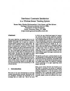
CERN, the laboratory for high-energy physics in Geneva, Switzerland, is currently engaged in a difficult and exciting enterprise, the realization of a new accelerator, the LHC 1 (see Figure 1.1). On completion, the LHC will be the most powerful instrument ever built to study the constituents of matter. Part of the LHC are 5 large-scale projects, the LHC machine, a 23 km accelerator ring and four particle physics experiments: ALICE, see Figure 1.2 2 , ATLAS 3 , CMS 4 and LHCb 5 . Each of these experiments is an independent project and is managed by a complex international collaboration of institutes. In this thesis, ALICE is taken as an example to study the technical integration and coordination issue of a distributed organisation. The ALICE collaboration is massive and involves more than 900 people from 80 institutes and 23 countries. Figure 1.4 depicts the ALICE collaboration with regards to the distribution of the personnel sent by the member countries. Each of the institutes is an autonomous organization and responsible for leading a subproject. A subproject in turn is defined by a large set of tasks and resources and represents essentially a resource constrained project scheduling problem. Budgets, manpower, spe1

LHC - Large Hadron Collider ALICE - A Large Ion Collider Experiment 3 ATLAS - A Toroidal LHC ApparatuS 4 CMS - Compact Muon Solenoid 5 LHCb - Large Hadron Collider beauty experiment 2

4


Figure 1.1: The LHC accelerator ring at the lake of Geneva, Switzerland.

Figure 1.2: The ALICE detector and its major subprojects.

1.2. The ALICE Experiment

5

cial tools, production units, manufacturing and assembly halls and cranes are the typical resources of a subproject schedule. Besides the resource constraints, the subproject schedules also contain temporal constraints such as deadlines and milestones, and precedence constraints that specify task sequences. A comprehensive introduction into general project management and practice can be found in the work of Kerzner [53]. Since the subprojects are interrelated by milestones, precedence and shared resources, the coordination of a subproject has two parts: the internal subproject coordination, ensuring the consistency of the tasks within the subproject, and the external subproject coordination, ensuring the consistency of the subproject to other subprojects, as well as to the general ALICE baseline schedule. Over the 15-year project horizon, the external coordination demands change. During the first 10 years, when the detector components are designed, engineered and manufactured at the institute sites, the subprojects are quasi independent of each other and the external coordination demand is very low. During the last 5 years however, when the detector becomes installed, the external subproject coordination demand increases dramatically. Figure 1.3 shows the summary of the ALICE installation schedule, which consists of approximately 1000 tasks. Once the project approaches this phase, it is likely that the number of tasks further increases. In this phase, the institutes deliver thousands of manufactured detector components, which need to be pre-assembled and tested before they are transported by two cranes into a 150-meter deep and narrow underground hall for final assembly and operation. The coordination of the installation phase with all the subprojects is extremely challenging and vital to ensure the timely completion of the ALICE project so that it is in step with the overall LHC programme. As Bachy and Hameri point out in their work [4], the technical integration and coordination of large scale projects such as ALICE which consists of multiple autonomous sub-projects is a great challenge. The difficulties are summarized as follows: Cultural Differences. The cultural differences amongst the institutes and the individual subproject planners are great and lead to a wide spectrum of heterogeneous schedules. The subproject schedules differ, for example, with regards to used project structures, the quality and reliability of scheduling data, the used planning items and methods, the used terms and semantics and also the used software tools. Privacy. The institutes keep their schedules private in order to protect themselves from external interference. The coordination of the schedules is achieved by exchanging and updating a limited amount of scheduling information, usually in the form of milestones. Due to long update delays, the subprojects are badly coordinated and inconsistent.

6


Self Interest. All subprojects have sub goals that sometimes conflict with those of other subprojects. Many of the sub goals are driven by self interest and often lead to a globally sub optimal schedule. Problem Distribution. Due to decentralized subproject leadership, schedule privacy and heterogeneous schedules, the subprojects are inherently distributed and schedules cannot be merged into a central coordination schedule. Problem Size. The size of the coordination problem is massive. The estimated number of tasks that will be executed within the 15-year project horizon, is 30,000. If we represent each task by only one variable, keep the duration fixed, and assume for each variable a temporal domain of 15 years with a resolution of 1 hour, the theoretical number of complete variable assignments would be astronomically large, (24·365·15)30,000 = 13140030,000 . Even if we centralise the problem and apply domain pruning and all kinds of consistency techniques, the problem remains intractably massive. Problem Dynamics. Although the number of institutes in the collaboration is almost constant for the entire project horizon, the problem itself is dynamic. Tasks, constraints and resources become continuously updated, added and removed as the project progresses and the schedules evolve. Problem Structure. The structure of schedules with regards to their tightness is not homogenous. Some parts of the schedule are tightly constrained or even overconstrained, whereas other parts are loosely constrained. Problem Consistency. The majority of the subproject planners develop schedules opportunistically and focus on local schedule consistency. The subproject external consistency very often is not given and possible flaws are discovered late. Another problem is the subproject internal and external resource consistency that is not supported by the used planning software.

1.3

Technical Challenges of Integrating Organisations

The cooperation, coordination and integration of organisations from the technical point of view is an ongoing research topic. The following points summarise some of the current challenges: Knowledge sharing. The majority of organisations maintain organically grown databases with inherent processes, data structures, terms and semantics. The merging of such heterogeneous information is always difficult and easily leads to ambiguities and miscommunication. It requires either standardisation or translation.

1.4. Distributed Constraint Satisfaction

7

Privacy. The majority of organisations need to keep operational data private as protection against competitors and fraud. This limits the possibilities to centralise operational data in order to synthesize consistent and efficient execution of interorganisational processes and tasks. Coordination. When companies cooperate, it usually involves the temporal coordination of resource and time constrained inter-organisational processes and tasks. When data centralisation is not possible, the coordination process must be distributed and achieved through partial information exchange. Distributed coordination is by several orders of magnitude harder to perform than centralised coordination. The reason being firstly, the complexity increase when information is distributed, secondly performance limitations given by the speed and reliability of the network and thirdly, high performing distributed coordination algorithms for large problems of thousands of variables and constraints do not exist.

1.4

Distributed Constraint Satisfaction

Distributed constraint satisfaction (see Yokoo et al. [113, 115]), unlike parallel problem solving, is not primarily concerned with efficiency. Distributed constraint satisfaction is concerned with solving inherently distributed problems, where the problem knowledge, the variables and the constraints, are distributed amongst the participating organisations and cannot be centralised, be it for transmission costs or privacy reasons. Distributed constraint satisfaction is therefore concerned with how to reach a solution from a given distributed situation. Distributed constraint satisfaction is still a young research discipline. The earliest papers appeared in the late 80’s / early 90’s and the largest body of work from the mid 90’s, after the pioneering work of Yokoo and his colleagues [114, 111, 116]. By the mid 90’s, many more papers appeared and it finally became a popular research topic. Over the last decade, distributed constraint satisfaction has made great progress. Several distributed complete, as well as local search algorithms were developed. Amongst the complete search algorithms are algorithms with asynchronous execution (Yokoo [117]), with distributed variable ordering schemes (Hamdi [43]), with distributed forward checking (Meseguer [66] and Meisels [64] and with arc consistency (Nguyen [75]). Amongst distributed local search algorithms are the distributed breakout algorithm (Yokoo et al. [116]), the distributed stochastic search algorithm (Zhang et al. [121]) and the distributed parallel constraint satisfaction algorithm (Fabiunke [25]). Besides the development of algorithms, other research issues were addressed. The following points summarise some of them: Solving Large Scale Problems. One of the biggest challenges of the DisCSP community is to develop algorithms that can handle problems of large-scale. Until now,

8


distributed systematic search algorithms have great difficulties to solve problems involving more than 30 variables in realistic time limits. Until now, no real world application has been reported where a DisCSP algorithm is used. One of the problems of complete DisCSP algorithms is the high number of messages when exploring problem sub spaces. Only distributed local search algorithms are capable of solving problems of a bigger size. However, their weakness is that of incompleteness: they can easily miss a solution and start to cycle. A big challenge of distributed constraint satisfaction is therefore to build algorithms that need fewer messages. Parallel Execution Protocols. Distributed constraint satisfaction problems are solved by several processors. When synchronous execution protocols are used, long idle times of the processor can occur, for example when the agent waits for a message. The wasted idle time could be used for parallel problem solving. Asynchronous protocols are a step in this direction. Other methods, divide the search space into subproblems, and solve these independently. Another challenge of distributed constraint satisfaction is to build algorithms that optimally utilize available processing capacity for solving the problem. Some work has been done on parallel execution, Zivan et al. [125] have proposed distributed parallel search, Hamadi [41] presented a distributed, interleaved, parallel, cooperative search algorithm. Dynamic Problem Context. Many practical DisCSP applications are situated in a dynamic (continuous) problem context, where variables, values and constraints are continuously added, removed and edited. In order to survive in these conditions, DisCSP algorithms should be built flexible, robust and allow the alteration of problem information, even during search. Relatively little work [44] has been done on solving DisCSPs in a dynamic context. Most work focuses on static contexts [115]. Disruptive Factors. When an application is distributed over a network, the probability of disruptions increases. Application nodes can be unavailable, long network delay times can occur, messages can arrive asynchronously in a different order than they were sent, and messages can be lost. In order to deal with these issues, DisCSP algorithms should be built flexible and robust. Asynchronous problem solving is one method to improve the algorithm flexibility. When an agent does not respond or his messages are lost, the remaining agents can continue to operate. In synchronous algorithms this is not possible, when a message is lost, the algorithm will stop. Another possibility is to choose a priory an algorithm, which is robust. Local search algorithms in general are robust and they seem to be the better choice when compared to complete search algorithms. Very robust local search algorithms are for example the distributed breakout algorithm [116], the distributed stochastic search algorithm [121, 27] and also the distributed parallel constraint satisfaction algorithm [25].


9

Privacy Requirements. One of the main reasons for developing DisCSP algorithms, is to keep information distributed and private. However, during search, some private information will always be revealed by consistent value assignments and inconsistent assignments, also referred to as nogoods. If the search takes long enough, private variables and constraints become more and more transparent. On the other side, agents can never tell if obtained domain information of another variable is complete. The domain can have more values, which are never selected because they would violate a constraint. Also, constraints are never directly revealed and a nogood is always highly summarised information, often the result of many constraints. Distributed local search algorithms have better privacy properties than distributed complete search algorithms. Distributed complete search algorithms explore the search space systematically, which makes the inferring of private knowledge easy. Distributed local search algorithms explore the search erratically and the inferring of private knowledge becomes difficult. The current challenge is to develop DisCSP algorithms that have better privacy properties. This does not only address the possibility to infer private knowledge, but also the security of data. Yokoo et al. [118] have developed a secure DisCSP algorithm that uses a public key encryption method to protect data. In this algorithm the problem is solved over a set of servers, which receive encrypted information from the agents. This algorithm is totally secure and does not leak any private information. The authors show that neither the agents nor the servers can obtain additional information on the value assignments of other variables of other agents. Other papers that also deal with privacy requirements can be found at [91, 66]. Autonomous Systems. A current research issue of distributed constraint satisfaction is also to build algorithms that have a degree of autonomy. Although we generally intend agents to act on our behalf, they should act without human intervention and have control over their internal state and actions. This property is desired to improve the flexibility, reliability and robustness of the system. For example, when an agent executing a DisCSP algorithm crashes, he should recover automatically without human intervention. Also the DisCSP system should be open, allowing the problem to define itself dynamically. Agents should be allowed to join and leave the problem context and search process. Discussions on openness in DisCSPs is given in [90, 12]. Data Heterogeneity. In DisCSP’s information is inherently distributed and the information providers are often from different organisations and have heterogenous data formats, representations and semantics. To exchange information under these conditions is difficult. The challenge of research is to develop data integration schemes that can overcome these difficulties using translation or standardisation methods.


10

1.5

Contributions

The main contributions of this thesis can be summarised by the following results: 1. The successful modelling, integration of a distributed, large-scale, heterogeneous, resource constrained, project scheduling problem of a large physics collaboration and solving the coordination problem with a distributed constraint satisfaction algorithm. For the first time a problem of such scale, consisting of thousands of variables, was solved with a DisCSP algorithm. Development of a prototype application of a multi-agent system. 2. The development of incremental problem solving scheme with variable ordering for local search algorithms. This scheme extends the search algorithm with a solution constructive element, where partial solutions are incrementally extended by selecting the next ordered variable and by assigning to it the first domain value, that is consistent with respect to the partial solution. In the best case the solution is constructed and no search is required. The scheme was implemented as central and as distributed local search algorithm. Empirical results prove that the scheme improves the algorithm performance dramatically for solving underconstrained problems. Since it is simple, its use is recommended for local search methods in general. At the same time, the execution protocol of the distributed breakout algorithm was improved. The neighborhood based change of assignment rule for competing proposals was replaced by an interference based rule, which is more relaxed and improves the concurrency properties of the algorithm. Empirical results show strong performance gains. 3. The development of a scheme for identifying hard or unsolvable subproblems and their ordering according to size. This scheme is based on the constraint weight information of the local breakout algorithm after the search and the graph structure. It is used to derive a constraint weight directed fail-first variable order, called CW, where the smallest hard or unsolvable subproblem is sorted to the top. Empirical results underline that this static fail-first variable order is ’perfect’. When it is used to guide simple backtracking, exceptionally hard problems do not occur, and, if the problem is unsolvable, the fail depth is always the shortest. The empirical results also prove that exceptionally hard problems are not a phenomenon of complete search algorithms in general, but are the result of imperfect variable ordering heuristics. The reason why problems become exceptionally hard is due to the sorting of variables of hard or unsolvable subproblems at positions, that are far apart in the variable list. Two hybrid algorithms that are complete, BOBT and BOBT-SUSP, were developed. BOBT combines the CW variable order with backtracking and, if the problem is unsolvable, it returns the first minimal unsolvable subproblem in the variable order. BOBT-SUSP combines the CW variable order with backtracking and, if the problem

1.6. Outline

11

is unsolvable, it returns the smallest unsolvable subproblem. The search for the smallest unsolvable subproblem is formalized as CSP and is supported by a powerful constraint weight sum constraint that substantially prunes the search space. 4. The development of a hybrid DisCSP algorithm called DisBOBT. This algorithm is the first hybrid DisCSP algorithm and combines local search, the distributed breakout algorithm with distributed complete search, distributed backtracking. The algorithm solves underconstrained problems with the distributed breakout algorithm (DisBO) and tightly or overconstrained problems with the distributed backtrack search (DisBT). It uses the CW variable order scheme to guide DisBT when the DisBO cannot find a solution after a bounded number of breakout steps. The CW variable order is incrementally determined, every time the partial solution needs to be extended the agents search for the next variable. Empirical results prove that the hybrid algorithm is very successful and reliably identifies unsolvable subproblems after few breakout steps. At this point it should be noted what this thesis does not address. No Optimisation. This thesis does not consider optimisation problems and primarily focuses on finding solutions. However, for future work, the coordination scheme could be extended towards optimisation by combining it with an incentive compatible auction process where the agents could pursue self interested goals. Only Depth First Search (DFS). This thesis only considers depth first search (DFS) algorithms [39, 86]. Due to the problem size, the memory requirement for implementing breath first search (BFS) is beyond realistic memory capacity. No Specialisation in Distributed Scheduling. Although this thesis deals with the integration of a distributed scheduling problem, the goal is not to develop new distributed scheduling techniques. The thesis is concerned with developing general methods for solving distributed constraint satisfaction problems.

1.6

Outline

The outline of this thesis is as follows. Chapter 2 summarises the related work on constraint satisfaction, distributed constraint satisfaction and scheduling. Chapter 3 contains the formalisation of the problem, introduces definitions, discusses the properties of unsolvable subproblems, and briefly recalls the execution of the breakout algorithm and the distributed breakout algorithm.


12

Chapter 4 is on the problem modelling, how the scheduling problem is represented as DisCSP and how information is translated unambiguously using a project ontology. Chapter 5 describes the incremental problem solving scheme with variable ordering and presents a central and distributed algorithm. Additionally a new interference based change of assignment rule for the distributed breakout algorithm is introduced. Experimental results that show significant performance improvements are presented. Chapter 6 describes a hybrid solving scheme for constraint satisfaction problems in general. Two hybrid algorithms are presented: • BOBT: Breakout Algorithm combined with Backtracking, as a complete mixed algorithm for solving CSPs or identifying an unsolvable subproblem if it exists, and • BOBT-SUSP: BOBT with the extension that it guarantees to identify the smallest unsolvable subproblem. The BOBT algorithm is evaluated by solving randomly generated graph 3-colouring problems. The results of the experiments are presented. A dynamic breakout step control is described and evaluated by comparing the BOBT algorithm performance with the dynamic breakout step control with static breakout step control. Related work is briefly surveyed. Chapter 7 applies the hybrid solving scheme of chapter 6 and presents a distributed hybrid algorithm for distributed constraint satisfaction problems. The results of the experiments are presented. Different algorithm variants which are based on the hybrid scheme are discussed and related work is briefly surveyed. Chapter 8 draws conclusions and outlines future work.

1.6. Outline

13

ALICE-Installation Schedule June 2002

ID 1

Start Wed 11/08/99

654

Mon 18/06/01

Finish Fri 07/10/05 Point 2 zone

655

Tue 01/01/02

Mon 08/01/07

656

Tue 01/01/02

Mon 27/01/03

657

Tue 01/01/02

Mon 12/08/02

Name

Tue 13/08/02 Mon 27/01/03

Mon 27/01/03

Tue 01/01/02

Mon 05/04/04

661

Tue 01/01/02

Mon 24/02/03

Crystal production

662

Tue 01/07/03

Mon 17/11/03

Assembly

Mon 27/01/03

Q3

Q4

2005 Q1

Q2

Q2

Q3

2007 Q1

Q4

Tue 18/11/03 Mon 05/04/04

Mon 05/04/04

Tue 25/02/03

Mon 09/08/04

Mon 05/04/04

Module 2

670

Tue 13/01/04

Mon 27/06/05

Module 3

675

Tue 30/11/04

Mon 03/04/06

Module 4

680

Tue 06/09/05

Mon 08/01/07

Module 5

685

Mon 17/12/01

Mon 27/02/06

686

Mon 17/12/01

Thu 01/04/04

Module 1 Crystal production 01/07

Assembly 18/11

Ready to install in UX25

Testing at CERN 05/04


/02

Module 2 13/01

Module 3 30/11

Module 4 06/09

Module 5

TPC pre-installation

TPC pre-installation

Construction TPC field cage (SXL2, 12m crane)

Wed 30/06/04

Mounting of chambers

Thu 01/07/04

Mon 03/01/05

Testing TPC/ITS/Va in SXL2

689

Mon 03/01/05

Mon 03/01/05

690

Tue 04/01/05

Mon 27/02/06

Testing TPC

691

Mon 27/02/06

Mon 27/02/06

TPC ready for installation In UX25

692

Mon 03/01/05

Tue 31/01/06

693

Mon 03/01/05

Mon 03/01/05

Start HMPID pre-installation

Construction TPC field cage (SXL2, 12m crane) Mounting of chambers Testing TPC/ITS/Va in SXL2 03/01

Start preinstallation of detectors in the Space-frame

Testing TPC 27/02

HMPID pre-installation

694

Tue 04/01/05

Tue 15/02/05

Mounting of cradle on space-frame

695

Wed 16/02/05

Thu 30/06/05

Mounting of modules on cradle

696

Thu 01/12/05

Thu 01/12/05

HMPID ready to install

697

Thu 01/12/05

Mon 30/01/06

Float

698

Tue 31/01/06

Tue 31/01/06

HMPID start of installation In UX25

699

Mon 03/01/05

Wed 05/04/06

700

Mon 03/01/05

Mon 03/01/05

Start TRD pre-installation

701

Tue 04/01/05

Wed 10/08/05

Mounting of TRD modules on space frame

03/01

HMPID pre-installation Start HMPID pre-installation Mounting of cradle on space-frame Mounting of modules on cradle 01/12 Float

Thu 15/09/05

Thu 15/09/05

Wed 05/04/06

Wed 05/04/06

704

Mon 03/01/05

Tue 01/08/06

705

Mon 03/01/05

Mon 03/01/05

Start TOF pre-installation

706

Tue 04/01/05

Thu 07/04/05

Mounting of TOF modules on space-frame

31/01

03/01

TRD pre-installation Start TRD pre-installation Mounting of TRD modules on space frame

50% TRD ready for installation in UX25

15/09

05/04

03/01

TOF pre-installation Start TOF pre-installation Mounting of TOF modules on space-frame

50% TOF ready for installation in UX25

15/07


Tue 01/08/06

Tue 01/08/06 Mon 12/06/06

710

Wed 30/06/04

Wed 30/06/04

Start ITS pre-installation

30/06

Start ITS pre-installation

711


30/06

ITS mechanics to CERN (including Pixel)

Wed 30/06/04

Wed 30/06/04

ITS mechanics to CERN (including Pixel)

Thu 01/07/04

Mon 03/01/05

Integration tests in SXL

713

Mon 03/01/05

Mon 03/01/05

Return ITS mech. to Turino

714

Mon 03/04/06

Mon 03/04/06

ITS ready to install date

715

Tue 04/04/06

Mon 12/06/06

Float

716

Mon 12/06/06

Mon 12/06/06

717

Mon 02/05/05

Fri 30/09/05

718

Mon 02/05/05

Mon 02/05/05

719

Mon 02/05/05

Fri 30/09/05 Fri 30/09/05

722

Tue 12/04/05

Tue 12/04/05

Tue 12/04/05

Tue 26/07/05

724

Tue 26/07/05

Tue 26/07/05

725

Mon 02/05/05

Fri 30/09/05

726

Mon 02/05/05

Mon 02/05/05

727

Mon 02/05/05

Fri 30/09/05

01/08

ITS pre-installation

712

Tue 26/07/05


03/01

Wed 30/06/04

Fri 30/09/05


100% TRD ready for installation in UX25 TOF pre-installation

709

Tue 12/04/05

HMPID start of installation In UX25

03/01

708

721

TPC ready for installation In UX25

03/01

TRD pre-installation

703

720

30/06

100% TOF ready for installation in UX25 ITS pre-installation

Integration tests in SXL 03/01

Return ITS mech. to Turino 03/04

ITS ready to install date Float

ITS (full detector) start of installation in UX25

12/06

PMD pre-installation

02/05

Start PMD pre-installation

02/05

Start PMD pre-installation

Pre-assembly work

Pre-assembly work 30/09

ZDC pre-installation

12/04

Start ZDC pre-installation

PMD ready for installation in UX25

ZDC pre-installation

12/04

Start ZDC pre-installation

Pre-assembly

Pre-assembly

ZDC ready for installation

26/07

FMD pre-installation

ZDC ready for installation

02/05

Start FMD pre-installation

FMD pre-installation

02/05

Start FMD pre-installation

Pre-assembly work

Fri 30/09/05

Fri 30/09/05

FMD ready for installation in UX25

729

Mon 18/06/01

Fri 01/04/05

MUON Chamber pre-installation

730

Mon 28/06/04

Mon 28/06/04

Pre-assembly work 30/09

Fri 01/10/04

Fri 01/10/04

732

Mon 18/06/01

Mon 18/06/01

Test / services / mech. ST3

733

Mon 01/11/04

Mon 01/11/04

ST3 ready for installation in UX25

734

Mon 29/11/04

Mon 29/11/04

Test / services / mech ST4, ST5,

735

Fri 01/04/05

Fri 01/04/05

736

Mon 29/11/04

Mon 29/11/04

Test / services / mech MT1 and MT2

737

Mon 03/01/05

Mon 03/01/05

MT1 and MT2 ready for installation in UX25

738

Wed 05/02/03

739

Fri 14/03/03

Wed 22/11/06

740

Fri 14/03/03

Fri 14/03/03

741

Wed 26/03/03

Thu 06/05/04

742

Wed 26/03/03

Thu 01/01/04

ASSEMBLY in UX25

746

Fri 02/01/04

Thu 06/05/04

Field Measurements (Dipole+L3 magnet)

751

Mon 17/03/03

Fri 08/10/04

752

Mon 17/03/03

Mon 28/06/04

757

Tue 29/06/04

Fri 08/10/04

FMD ready for installation in UX25

MUON Chamber pre-installation

Test / services / mech. ST1, ST2

731

ITS (full detector) start of installation in UX25

PMD pre-installation

PMD ready for installation in UX25

728

28/06

ST1, ST2 ready for installation in UX25

Test / services / mech. ST1, ST2 01/10

ST1, ST2 ready for installation in UX25

01/11

ST3 ready for installation in UX25

29/11

Test / services / mech ST4, ST5,

29/11

Test / services / mech MT1 and MT2

ST4, ST5, ready for installation in UX25

01/04

03/01

ST4, ST5, ready for installation in UX25

MT1 and MT2 ready for installation in UX25

Thu 01/03/07 ALICE Installation Muon Arm Installation Start Muon arm installation

Absorber Installation Front Absorber

Fri 27/08/04

Thu 30/12/04

Muon Filter / Superstructure Installation

Tue 14/09/04

Mon 21/02/05

Infrastructure

773

Mon 29/11/04

Tue 12/07/05

Tracking Chambers Installation

779

Mon 03/01/05

Tue 12/07/05

Trigger Chambers Installation

786

Wed 08/11/06

Wed 22/11/06

PMD Installation

790

Mon 28/06/04

Mon 06/02/06

PHOS Installation Phase 1

798

Mon 08/01/07

Thu 01/03/07


804

Wed 05/02/03

Thu 15/12/05

Space-frame / Baby space-frame

822

Tue 31/01/06

Tue 18/04/06

HMPID Installation

832

Fri 15/07/05

Thu 08/09/05

TOF Installation Phase 1

837

Wed 08/11/06

Wed 20/12/06


843

Thu 15/09/05

Wed 09/11/05

TRD Installation Phase 1

848

Wed 05/04/06

Tue 06/06/06


Tue 02/05/06

Wed 08/11/06

Wed 08/11/06

Wed 08/11/06

868

Wed 14/06/06

Wed 18/10/06

880

Tue 27/06/06

Tue 08/08/06

891

4/03

Muon Arm Installation Start Muon arm installation Dipole Magnet Installation ASSEMBLY in UX25 Field Measurements (Dipole+L3 magnet)

7/03

Absorber Installation

7/03

Front Absorber

Small Angle Absorber

767

867

ALICE Installation 4/03

Dipole Magnet Installation

761

854

Q3


Testing at CERN

688

Fri 15/07/05

Q2

Production


665

723

2006 Q4 Q1 Point 2 zone

Q3

PHOS pre-installation /

Production

664

Fri 15/07/05

Q2

Cradle

Module 1

663

707

2004 Q1

Q4

Design

660

702

Q3

ALICE Pre-Installation i

Cradle

659

Fri 02/04/04

Q2

PHOS pre-installation / production

658

687

2003 Q1

Mon 08/01/07 ALICE Pre-Installation in the SXL2 Hall

Small Angle Absorber 27/08

Muon Filter / Superstructure Installation

14/09

Infrastructure 29/11 03/01

Tracking Chambers Installation Trigger Chambers Installation 08/11

28/06

08/01

HMPID Installation

TOF Installation Phase 1 08/11 15/09

05/04


02/05

TPC Installation 08/11

ITS Installation

14/06

Vacuum Chamber Installation

Tue 08/08/06

Wed 29/11/06

FMD/T0/V0 Installation

Fri 01/10/04

Wed 19/10/05

ZDC Installation

Tue 01/11/05

Tue 06/02/07

923

Tue 06/02/07

Tue 06/02/07 ALICE INSTALLATION COMPLETED

924

Fri 30/03/07

MACHINE INTERFACE Installation

Fri 30/03/07 LHC SCHEDULE

Installation 2nd Phase ITS Installation

27/06 08/08 01/10



Installation 2nd Phase

908

PHOS Installation

Space-frame / Baby space-frame 31/01

TPC Installation

900

PMD Installation


Vacuum Chamber Installation FMD/T0/V0 Installation

ZDC Installation 01/11

MACHINE INTERFAC 06/02

ALICE INSTALLATIO 30/03

Figure 1.3: Summary of the ALICE installation schedule, which consists of nearly 1000 tasks.

M e m b e r s

Figure 1.4: The ALICE collaboration.

Members

LoI

Italy

JINR

France

PHOS HMPIDTDR

Year

Russia

Sweden Greece UK Hungary Portugal Netherlands

Poland

Czech Rep. Norway

Slovak Rep.

Denmark

CERN

Finland

Germany

ALICE Collaboration

MoU

Muon TDR TP TP

Mexico

Armenia Ukraine

India

China Croatia

Romania USA

Collaboration Statistics

Institutes

Countries

(64% from CERN MS)

1992 1993 1993 1994 1995 1995 1996 1997 1997 1998 1999 1999 2000

0

100

200

300

400

500

600

700

800

900

1000

27 73

912

14


Chapter 2

Related Work 2.1

Constraint Satisfaction

One of the major concerns of Artificial Intelligence (AI) is to solve problems, see for example the works of Simon [93], Wallace [106], Norvig [76] and Russel et al. [86]). Solving problems invariably means to search through a vast maze of possibilities and successful problem solving involves searching that maze selectively and reducing it to manageable proportions. The Artificial Intelligence community has come up with a widely accepted standard definition for defining search problems, called Constraint Satisfaction Problems (CSP). A brief introduction to CSP and techniques can be found in the work of Bartak [6]. Also, the work of Dechter [16] gives a comprehensive and detailed summary of CSP and the work of Stucky [62] concentrates on programming aspects of CSPs. Informally, a CSP problem is defined by the triple < X, D, C >, see Definition 3.1, where X is a set of variables, D is a set of domains and C is a set of constraints. CSPs have a long history in Artificial Intelligence, see for example [61]. The CSP definition is very expressive and powerful and it facilitates the formalisation of a wide range of search problems and applications [105]. Solving a CSP means to search through all possible assignments until a solution is found. Existing search methods fall into two categories:

• Systematic search, where a complete assignment is constructed variable by variable. • Local search, where search moves from one complete assignment to the next and is guided by the complete assignments.

Chapter 2. Related Work

16

2.1.1

Systematic Search Methods

Systematic search methods are usually designed to explore the entire search space and guarantee completeness. If a solution exists, systematic search will find it, or prove that no solution exists. A weak point of systematic search methods however, is to get caught in dead-end branches, when an inconsistent value is assigned to one of the first variables of the search tree and causes exhaustive search. Backtracking. Backtrack search is a systematic search method and is used for a depthfirst search (Russel and Norvig [86]) that chooses values for one variable at a time and backtracks when a variable has no consistent values left to assign. Backtracking goes back to the work of [45]. A good summary and evaluation on different backtracking algorithms is given in Dechter et al. [17]. The performance of simple backtracking can be improved by a number of techniques. Backjumping (Gaschnig [32]) for example is a technique to reduce the rediscovery of the same dead-ends. Instead of backtracking to the last variable in the search tree, it jumps back to the most recent variable in the conflict set. Conflict directed backjumping (Prosser [84]) is a refined version of backjumping and uses conflict sets. A good survey for different backjumping variations is given in the work of Dechter et al. [18]. Variable Ordering. Variable ordering is another very important technique to improve the performance of systematic search. In general, a variable order is good if the hardest part of the problem is solved first as it can maximally limit further search. A good overview on dynamic variable ordering is given in [3]. Amongst the variable ordering heuristics, the MRV heuristic (minimum remaining values) is very successful and used for a large number of problems. The MRV heuristic is also known as failfirst, or most constrained variable heuristic, as it selects a variable that is most likely to fail next. The MRV variable order goes back to the work of Bitner and Reingold [10]. Value Ordering. Value ordering techniques, also referred to as value selection techniques, focus on the order in which to assign values to the variable. One good strategy is to choose the least constraining value as the next value. This value ordering technique is known as least-constraining-value heuristic and was proposed by Haralick and Elliot [45]. A number of other value ordering techniques are presented in [88, 2, 16], [16] Consistency Algorithms. The earliest works on consistency algorithms go back to Waltz [107]. Consistency algorithms (see Mackworth [61]) are preprocessing algorithms that prune the search space by propagating the implications of a constraint on one variable onto other variables. The simplest form of consistency algorithm is forward checking (see McGregor [63], Haralick [45] and Bacchus et al. [2]).

2.1. Constraint Satisfaction

17

Every time a variable x is assigned a value, the forward checking process checks on the impact on the unassigned variables that are constrained with x and deletes the domain values that are inconsistent with the assignment of x. If a domain becomes empty, x is assigned the next domain value. A very successful, more sophisticated consistency algorithm is arc consistency. Arc consistency goes back to the work of Waltz [107] who solved polyhedral line-labelling problems for computer vision and Mackworth [60] who proposed the AC-1, AC-2 and AC-3 algorithm for enforcing arc-consistency and developed the idea to combine it with backtracking. The idea of arc consistency is to ensure that each domain value of a variable x is supported by at least one domain value of each neighbour variable, which has a constraint with x. AC-4 a more efficient arc consistency algorithm, was developed by Mohr and Henderson [71]. Formally, arc consistency can be achieved by the following domain restriction operation: ∀(i, j) ∈ arc(G) : Di ← {v|v ∈ Di ∧ ∃w ∈ Dj : Cij (v, w)}. Arc consistency is sometimes referred to as 2-consistency as it applies to two variables. Further important arc consistency algorithms can be found by Sabin and Freuder [87] and Bessiére [9]. Montanari [72] introduced the notion of path consistency, also referred as 3consistency, which means that any pair of variables, connected by a constraint, can always be extended to a third neighbouring variable. The most general consistency algorithms, are called k-consistency algorithms, where k specifies the consistency depth of a given variable. K-consistency was introduced by Freuder [29, 30]: a CSP is called k-consistent if, for any set of k - 1 variables and for any consistent assignment to those variables, a consistent value can always be assigned to any k th variable.

2.1.2

Local Search Methods

Local search methods are designed to explore the search space in a non systematic way. This usually is performed by moving from one state to a neighbouring state, where a state represents a total value assignment for all variables, and a neighbouring state represents an assignment that usually differs by only one variable value assignment. Local search algorithms in comparison to systematic search algorithms usually have much easier execution protocols, cannot get stuck in dead-end branches and have very low memory requirements as they do not maintain a search tree. One of the major drawbacks of local search is the lack of a completeness guarantee, which means that local search algorithms cannot guarantee to find a solution if one exists, and also end up in infinite execution cycles if no solution exists. Hill-Climbing. Hill-climbing, also sometimes called greedy local search, works with complete variable value assignments and an evaluation function, that evaluates all pos-

18


sible neighbouring states that can be reached from the current state. Hill-climbing usually starts from a random assignment and moves to the neighbouring state with the best evaluation value until a goal state is reached or until the algorithm gets caught in a local minimum. In case of such local minima the algorithm is usually restarted. Hill-climbing example algorithms can be found in the works of O’Reilly et al. [77]. Min-Conflict. The min-conflict heuristic [68] is a hill-climbing variation, where the heuristic iteratively tries to minimize the number of conflicts by assigning new values to the variables. Ties are broken randomly, and when the heuristic gets stuck in a local minimum then it causes a restart with a new random assignment. A variation of the min-conflict heuristic is the breakout algorithm, see Morris [73]. Tabu Search. Tabu search is another hill-climbing variation. When the heuristic gets stuck in a local minimum, the algorithm memorises the local minimum state in a so called tabu list and moves to a neighbouring state. Then this memorised state cannot be visited for the next k-moves. Examples of tabu search algorithms can be found in the works of Glover [36, 37]. Simulated Annealing. Simulated annealing [54] is another hill-climbing variation and motivated by solid state physics. In this algorithm we choose moves according to a probability distribution over available moves and we favor moves to nodes having lower elevation. If the move improves the situation, it is always accepted. Otherwise, the algorithm accepts the move with some probability p < 1. This probability decreases over time and the parameter that controls it, is often called the temperature. The algorithm got its name by analogy with the annealing process in metallurgy. Genetic Algorithm. Genetic algorithms are evolutionary search methods. In these algorithms, the successor states are generated by combining two parent states. At the beginning, the algorithm generates k random states, called the population. Then in order to generate the next population, two states, also referred to as strings, are randomly selected and combined with a crossover point. The crossover point defines which part of each string (state) is used for the new, combined string. From a large set of such newly combined states the fittest states are selected for generating the next population. The states (strings) are also subject to random mutation. A great deal of information about genetic algorithms can be found in the works of Goldberg [38], Mitchell [69] and Fogel [28]. Guided Local Search. Guided local search (GLS) (Voudouris et al. [103, 104]) is another hill-climbing variation, which augments the objective function with penalties in order to help hill-climbing to escape from local minima. The penalties refer to


19

features exhibited in the candidate solution and aim to avoid these features for future states. Guided local search is very successful for applications such as function optimization, large scale scheduling and the travelling salesman problem.

2.2

Distributed Constraint Satisfaction

In distributed constraint satisfaction problems, variables and constraints are distributed amongst a set of automated agents. A solution of a DisCSP, is a value assignment for all variables, that satisfies all constraints. Various applications have been modelled as DisCSPs, such as distributed resource allocation problems [14], distributed scheduling problems [97, 22, 21], distributed sensor networks [120] and multi-agent truth maintenance tasks [51]. Analogue to CSPs, algorithms for Distributed Constraint Satisfaction Problems (DisCSP) also fall into two categories: distributed systematic and distributed local search algorithms.

2.2.1

Challenges

The challenges for distributed constraint satisfaction problems are the same than for central CSPs. In addition, when solving DisCSP problems, new challenges arise with regards to message synchronization, traffic and disruptions, the extended problem complexity due to the inherent problem distribution and also data privacy. Synchronization. In real distributed problems where the DisCSP must be solved over a network or even the Internet, the timely arrival of messages cannot be guaranteed. Due to network delays and asynchronous operation, messages can be delayed and arrive in a different sequence than when they are sent. DisCSP algorithms therefore must cope with message delay and asynchronous message sequences. Message traffic. The temporal bottleneck of central CSP algorithms is usually the delay time caused by constraint checks. In DisCSP algorithms however, where variables are distributed, the constraint checks are often combined with message exchange. The delay time of sending a message, in the worst case when it is sent over the internet, is by order of magnitudes greater than that of a constraint check performed in the CPU. Therefore a big challenge of DisCSP algorithms is to reduce the message traffic. This goal can be achieved by either packing more information into each message or by designing coordination protocols that require fewer constraint checks for constraints between distributed variables. Problem distribution. By the DisCSP definition, not all variables and constraints of the problem are visible to all agents. Some problem parts are public, others are private. This complicates the solving process and leads to bad efficiency. When


20

an agent does not have the total view of the problem, he can propose to label a variable with a value that is a priori incompatible with a private variable of another agent. The inconsistency then must be communicated by a message. In central search algorithms such inconsistent labelling can be easily detected and avoided by simple forward checking or propagation techniques. Parallelism. One advantage of DisCSP over CSP algorithms is that more processing power is available since the problem is solved by multiple processors units. However, due to delay times of the network, the bottleneck is seldom the processing power. The goal of future research should therefore address the development of algorithms that can better utilize available processing power that is idle during the algorithm execution. These challenges require the development of new solving strategies, tailor made for solving DisCSPs. One of the major challenges for these strategies is to develop techniques that reduce the number of messages. One such method, which current research work has not explored in great depth, is to use fixed assignment rules for labelling variables. Fixed assignment rules restrict the agents to only assign values that are compatible to all the restricted values that can be assigned to a neighbour variable of another agent. Such an assignment rule can be realised by dividing the variable domain values into two groups of compatible and non compatible values. If the agent finds a consistent value amongst the compatible values, then a consistency check is not necessary and a message can be saved. If however, no compatible value is available then the agents will have to perform the consistency check and send messages. Such a simple assignment rule is used in the distributed parallel constraint satisfaction algorithm from Fabiunke [25] for solving distributed job shop scheduling problems. In this algorithm the agents select their variable values using two independent rules. By applying the first rule, which is a task shifting rule, the agents move their conflicting tasks in a coordinated way to new positions, which will not create a new conflict with the same tasks. Only when a new conflict cannot be avoided, then the second rule applies. With the second rule, the agents move their tasks to a new, min-conflict position with a certain probability. Fabiunke’s results prove that such rules are very successful, especially when they are applied for solving underconstrained problems. Therefore the development of further rules is a promising research direction.

2.2.2 2.2.2.1

Distributed Systematic Search Methods Distributed Backtracking

Synchronous Distributed Backtracking (DBT). The synchronous distributed backtracking algorithm was developed by Yokoo et al. [114, 115, 113]. This algorithm is the simplest systematic and complete search algorithm for distributed constraint satisfaction problems and is based on simple backtracking. In this algorithm each agent


21

has exactly one variable. Not that this condition applies for most DisCSP algorithms in order to simplify the algorithm description. Specific to DBT is that the agents agree on a fixed variable order and pass to each other a growing partial assignment until the problem is solved. When the agent receives a partial assignment he tries to assign a value to his variable. If this is successful the new partial assignment with the new variable value is passed onto the next agent. If no value is consistent with the partial assignment, then the agent sends a backtracking message back to the agent that had sent the partial assignment. A weakness of this algorithm is that it cannot take advantage of parallelism, the problem is solved synchronously and only one agent can process a variable at a time. Another problem of this algorithm is the static variable order, which must be determined beforehand and thus involves an extra computational cost. During algorithm execution, the variable order cannot change. Asynchronous Backtracking Algorithm(ABT). The asynchronous distributed backtracking algorithm was developed by Yokoo et al. ([114, 115, 113]). ABT is an asynchronous version of DBT, where the agents process their variables concurrently and asynchronously. During the execution the agents instantiate their variables concurrently and send ok? messages to all agents that have a constraint with their variable, in order to request, if the value is consistent. If this value is not consistent, the value receiving agent will reply with a nogood message to the value sending agent. Each agent also keeps an agent view object, which holds the current assignment of the neighbour variables and it is used by the agent to check if his own variable assignment is consistent. A total variable order is used for avoiding infinite processing loops. The agent that has the lower priority will always be an evaluator and the agent that has the higher priority, will always send a value. Yokoo et.al. show that ABT is complete and that it has in the worst case an exponential time complexity but no exponential space complexity. The nogoods, which define the space complexity, can be deleted and the agent must store at most |Di | nogoods, where |Di | is the domain size of the variable xi . A weakness of ABT is the static priority (variable) order, which must be determined beforehand. If this priority order sorts the ’wrong’ variable to the top of the priority order, the search space easily becomes exponentially large. Also, in the worst case, asynchronous problem solving can lead to a redundant exploration of the search space and becomes a source of expensive message exchange and can require exponential memory for nogood recording. Distributed Backtracking Algorithm (DIBT). [43] Hamdi et al. have developed an advanced asynchronous distributed backtracking algorithm, where conflict directed backjumping [18] and a general distributed variable ordering scheme for static variable ordering is implemented. In contrast to ABT, this algorithm does not record nogoods and performs exhaustive search. In the experiments a max-degree variable

22


order was used and the method was compared with standard distributed backtracking. The experiments showed that DIBT outperforms DBT for all problem regions what concerns, number of constraints checks, number of messages and average time to solution. A weakness of this algorithm is that it uses a static variable order and, although the authors claim that it is complete, it is actually incomplete (see [8]). Asynchronous Weak Commitment Search Algorithm (AWCS). The asynchronous weak commitment search algorithm was developed by Yokoo ([112, 113, 115]) and goes back to the weak commitment search algorithm for CSP [111]. AWCS is essentially a further development of ABT with the novelty that the agents dynamically change their priority order (variable order) in order to prevent exhaustive search. The priority change works as follows, when a lower priority agent cannot find a consistent value with regards to higher priority agents, the priority order is changed and the lower priority agent gets the highest priority amongst these agents. This means that when an agent has made a mistake by assigning a value to his variable that is not consistent with the value assignments of the other agents, another agent will get a higher priority and the agent will change the assignment and not commit to the bad decision. Another important characteristic of AWCS is the use of a min-conflict value ordering heuristic (see [68]), where the agent always chooses from the consistent values with regards to higher priority agents, the one, which implies the least number of constraint violations with regards to lower priority agents. A weakness of AWCS is that it has exponential complexity due to nogood recording in order to guarantee completeness. Unlike ABT, it cannot discard recorded nogood’s. Distributed Dynamic Backtracking Algorithm (DisDB). The distributed dynamic backtracking algorithm was developed by Bessiére et al. [8] and was designed to take the best of ABT and DIBT. The algorithm is an asynchronous, complete search algorithm and tries to minimize the number of messages. Like DIBT it performs dynamic jumps over the set of conflicting agents and it uses the same distributed static variable order method. In order to ensure completeness, it performs nogood recording and keeps an agent view. The implied space complexity is only polynomial as nogoods can be discarded. The experiments show that DisDB is only marginally better than ABT. Conflict directed backjumping which saves a great deal of messages is responsible for the performance gain. Distributed Parallel Backtracking Algorithm. A distributed parallel backtracking algorithm was developed by Zivan et al. [125]. This algorithm performs parallel search on interleaving subtrees (see Meseguer et al. [65]). The subtrees are generated from the main tree by dividing it by the possible assignments of the first variable. Distributed, Interleaved, Parallel and Cooperative Search. The distributed, inter-


23

leaved, parallel and cooperative search algorithm was developed by Hamadi [42]. This method was developed for efficiency reasons, and combines distributed interleaved and distributed parallel search. The implemented backtracking search is sequential conflict-directed backjumping [83, 18] and implements a filter technique. Detected conflict sets can remove inconsistent values between agents. The algorithm is evaluated by solving a large set of random CSPs, the shape of the phase transition is presented. More work in distributed backtracking includes Fox and Sycara [97] who developed an incomplete backjumping based heuristic search algorithm and Solotorevsky et al. [96] who developed a complete algorithm that deals with problems that consist of one central and many peripheral problems. 2.2.2.2

Distributed Arc-Consistency

Distributed Arc Consistency. A distributed arc consistency algorithm was presented by Nguyen et al. [75]. This algorithm is based on AC4 [71], is complete and has a parallel execution protocol designed for distributed memory computers. Another consistency algorithm for asynchronous distributed algorithms such as ABT was presented by Silaghi et al. [92]. This algorithm is complete, has polynomial space complexity, generalizes distributed forward checking and if implemented in ABT can exploit available backtracking nogoods for better maintained consistency. Distributed Forward Checking. An early distributed forward checking algorithm was presented by Meseguer et al. [66]. This algorithm is combined with distributed backtracking. Although it cannot improve the backtracking efficiency since the ability to accumulate pruning on future domains gets lost, the algorithm supports total privacy. Every agent knows his own value but not the other agents values. Another Distributed Forward Checking algorithm, with dynamic variable ordering, was developed by Meisels et al. [64]. The novelty of this algorithm is that it dynamically orders variables during search. The dynamic variable ordering is realised by agents which propose variables and values to each other, evaluate these and take a cooperative decision. Analogue to [64] the algorithm is complete and has the same privacy properties. Asynchronous Aggregation Search (AAS). The asynchronous aggregation search algorithm was developed by Silaghi et al. [91] and contributed two novelties. The first addressed the separation between public and private information. In traditional DisCSP algorithms, constraints are public and variables are private, in AAS the situation is reversed, constraints are private and variables are public. The second novelty addressed the search technique, which differs from other DisCSP search


24

methods in that it treats sets of partial solutions and exchanges messages on aggregated valuations for combination of variables. 2.2.2.3

Distributed Constraint Satisfaction and Optimisation

Distributed Partial Constraint Satisfaction. Distributed partial constraint satisfaction (DisPCSP) deals with overconstrained problems and the goal is to find a consistent assignment to an allowable relaxed problem. Hirayama et al. [48] provide a formal framework for overconstrained distributed CSPs. In their work they describe two algorithms, synchronous branch and bound (SBB) and iterative distributed breakout (IDB) for solving distributed maximal constraint satisfaction problems (DisMCSPs), an important subclass of DisPCSPs. The algorithms are evaluated with random CSPs. The experiments show that SBB always finds the optimum but not IDB. However, to get quickly to a nearly optimal solution, IDB is better. Adopt. Adopt (An Asynchronous Complete Method for Distributed Constraint Optimization) was proposed by Modi et al. [70]. This algorithm guarantees to find an optimal solution or a solution within a user-defined distance from the optimal. The algorithm is executed asynchronously and in parallel. The space complexity is only polynomial. In this algorithm agents perform distributed backtrack search by locally exploring partial solutions asynchronously. The algorithm has a built in termination detection. Speedups are achieved by three novelties, firstly, an ’opportunistic’ bestfirst search strategy where the agent can choose the best value based on the current information, secondly, to allow agents to efficiently reconstruct a previously explored solution and thirdly, by using bound intervals for tracking the progress towards the optimal solution. The algorithm obtains significant speedups over distributed branch and bound search. A Broker Model for DisCSOP. Lin develops a broker model for distributed constraint satisfaction and optimisation [59]. In this method the agents firstly solve their own CSOP problem and then deallocate the non-optimized variables according to a deallocation procedure. These variables are then sent to the central agent, namely the broker, who collects the non-optimized variables from all agents. These nonoptimized variables as a whole represent a subproblem, that the broker agent optimizes. The aggregation of the partial solutions from all the agents and the broker then give a global solution.

2.2.3

Distributed Local Search Methods

Distributed local search methods generally have much simpler execution protocols than distributed complete search methods. Several distributed local search methods are developed.


25

Distributed Breakout Algorithm (DisBO). The distributed breakout algorithm was implemented for the first time by Yokoo et al. in 1996 [116]. In this early work two algorithm versions were presented. One works with quasi-local minima, the other with global minima. Though the quasi local minimum version required on average more algorithm cycles to get to the solution, it required 10 times less messages than the real local minimum version where the expensive broadcasting method is used for detecting the local minimum. DisBO was further investigated by Zhang et al. [122]. The authors could prove that the algorithm is complete for solving problems with an acyclic graphs (trees) structure. It was shown that DisBO guarantees to find a solution in less or equal to O(n2 ) steps for acyclic graphs with n nodes. The authors argue that the completeness property explains the superiority of DisBO over many other local search algorithms. Furthermore, in the paper two variants of DisBO are implemented. These variants have stochastic properties, the variable value assignments are changed with a probability. The stochastic variants show small performance improvements over DisBO. Distributed Stochastic Search Algorithm (DSA). Zhang et al. present the distributed stochastic search algorithm DSA [121, 120, 124, 123] for solving sensor network problems. An early work relating to stochastic search can be found by Pearl [81]. The DSA algorithm is uniform [99], all processes are equal and no feature distinguishes one from the other. In comparison, DisBO is not uniform, in this algorithm agents use priority rules for decisions in tie breaking situations. The synchronous execution protocol of DSA is very simple. It has an initial step where the agents randomly select a value for their variables. Then the agents go through a sequence of steps until a termination condition is met. In each of these steps, the agent updates his neighbours on his variable value and receives the value updates from his neighbours. Then the agent decides to keep the value assignment or change it. The decision process is often stochastic, based on the current state of the agent and the believed states of its neighbours. The long term goal of the decision process is to reduce possible constraint violations. Different decision strategies yield different DSA variations. Zhang et al. compare DSA with DisBO [121] and conclude that a modified version of DSA, called DSA-B, which has a higher degree of parallel actions than the standard version, outperforms DisBO, including tightly and overconstrained problems. In another work [124], Zhang et al. solve distributed scan scheduling problems with DisBO and DSA and compare their performance. The results show that DSA is superior to DisBO, it provides better solution quality and lower communication costs.


26

The DisBO communication costs are constant for each cycle and either equal or greater than that of DSAs. DSAs communication costs depend on the number of variables that violate a constraint, when DSA progresses to the solution the communication costs go down. For the distributed scan scheduling application the authors prefer DSA over DisBO. Distributed Parallel Constraint Satisfaction (DPA). Fabiunke developed a parallel distributed constraint satisfaction algorithm [25] that was motivated by a connectionist method for neural networks [98, 1]. The execution protocol of this algorithm is entirely parallel, asynchronous and very simple. The agent first initializes its variables and updates his neighbours on this value. Then the agent goes through a number of steps until the termination condition is met. In each of the steps the agent revises its variable assignment in the spirit of the min-conflict heuristic [68]. If the assignment has changed, the neighbours are updated on the new value. In order to prevent the algorithm to oscillate, e.g. two agents keep changing the assignment of their conflicting variables into the same ’direction’, always causing a new violation, an additional value assignment rules is introduced. This rule breaks the symmetry of the variable value assignment rule, it states that when the agent detects a constraint violation he applies the min-conflict rule only with the probability p. The difference between DPA and DSA algorithms are the parallel and asynchronous features of DPA. In DPA the agents do not wait for variable value update messages of their neighbours and change the variable value assignment as soon as possible. Also the probabilistic rule for changing a variable value assignment is different in the two algorithms. DPA is really an autonomous protocol, the agents do not wait for other agents and achieve a high degree of parallelism and asynchronism. DSA algorithms are more coordinated, they have a synchronous protocol and a more refined, cooperative change of assignment rule. For building robust, autonomous and self-stabilizing applications, DPA is the better choice, however the performance is probably not as good as that of DSA algorithms.

2.3 2.3.1

Scheduling Resource Constrained Project Scheduling Problems

The ALICE coordination problem belongs to the class of Distributed Resource Constraint Project Scheduling Problems (RCPSPs). A good introduction from the Operations Research (OR) community into this problem class is given by Klein ([55]). More works concerning the mathematical properties can be found in the work of Bartusch et al. [7]. The work of Hildum ([47]) studies the RCPSP in dynamic environments and develops schemes and algorithms with greater flexibility.

2.4. Agents

2.3.2

27

Distributed Scheduling

A distributed scheduling problem is described in the work of Sycara et al. [97], it deals with a multi agent resource allocation problem. Another interesting work can be found with Dusseau et al. [20] who implement a distributed algorithm for time-sharing parallel workloads that is competitive with co-scheduling.

2.4

Agents

In this thesis the distributed project scheduling problem is coordinated by a finite set of agents. In this setting, each agent represents an institute. An agent is defined as an autonomous computer system, capable of acting independently in an environment and exhibiting control over its internal state. An intelligent agent is a computer system capable of flexible autonomous action in some environment, where flexible means reactive, proactive and social behaviour. A more detailed introduction into intelligent agents and multi-agent system can be found in the works of Woolridge et al. [110, 109], Panzarasa et al. [80] and also in [108, 52].

Chapter 3

Formalization 3.1

Definitions

Definition 3.1 (Constraint Satisfaction Problem P ) . A finite, binary constraint satisfaction problem is a tuple P =< X, D, C > where: • X = {x1 , .., xn } is a set of n variables, • D = {d1 (x1 ), .., dn (xn )} is a set of n domains, and • C = {c1 , .., cp } is a set of p constraints, where each constraint cl (xi , xj ) involves two variables xi and xj and is a function from the Cartesian product di (xi ) × dj (xj ) to {0, 1} that returns 0 whenever the value combination for xi and xj is allowed, and 1 otherwise (note that this is the formulation of weighted CSP). We call the set {xi , xj } vars(c) and there is at most one constraint with the same set of variables. Solving a CSP is equivalent to finding a simultaneous variable value assignment S, which satisfies all constraints in C. CSP’s are NP complete in general, that is, no algorithm is known which guarantees to solve the problem in polynomial time ([31]). CSPs are usually solved by trial and error search, where value assignments are generated in a systematic or non systematic way and verified if they satisfy the constraints of the problem. Besides the goal to solve a CSPs, sometimes optimization is needed, which means to select the best solution from all solution alternatives. For this purpose, CSP’s are then extended by a cost function for evaluating and comparing solutions. In this work however, we are not concerned with optimisation questions. Definition 3.2 (Subproblem Pk ) . A subproblem Pk of a problem P with k variables is defined as a tuple Pk =< XPk ⊆ X, DPk ⊆ D, CPk ⊆ C > with the additional property that CPk contains all and only constraints between variables in XPk . We define the size of a subproblem as the number of constraints |CPk |.

Chapter 3. Formalization

30

Definition 3.3 (Unsolvable Subproblems usp) . A subproblem Pk is unsolvable if there is no value assignment to variables in XPk that satisfies all constraints in CPk . An unsolvable subproblem Pk is minimal if it becomes solvable by removing any one of its variables. A minimal unsolvable subproblem Pk is a smallest unsolvable subproblem of P , if there is not another minimal unsolvable subproblem Pl0 such that size(Pl0 ) < size(Pk ). Definition 3.4 (Graph Connectivity GC) . The connectivity of a variable is the number of constraints which refer to that variable. The connectivity of a graph GC is the average connectivity of the variables. See ([33]). Definition 3.5 (Distributed Constraint Satisfaction Problem (DisCSP) Pdis ) . A distributed constraint satisfaction problem Pdis is a Constraint Satisfaction Problem where the variables, domains and constraints are distributed amongst a set of s agents. A = {a1 , .., as }. Solving a CSP and DisCSP is equivalent to finding a value assignment for all variables, that simultaneously satisfies all the constraints in C. In our model each agent owns multiple variables, and distinguishes between private and public variables. Definition 3.6 (Private and Public Variables) . • Private variables are only visible to the owner agent and are not part of any public constraint. ∀xi ∈ Xpriv (¬∃cj (xk , xl ) ∈ Cpub ∧ (xi = xk ∨ xi = xl )). • Public variables are visible to all agents and are part of one or more public constraints. ∀xi ∈ Xpub (∃ci (xj , xk ) ∈ Cpub ∧ (xi = xj ∨ xi = xk )). In this context we also define the function Owner(xi ), which returns the owner agent of xi . Note that we assume in this thesis that all variables of the CSP problem graph are connected and do not contain any independent subproblems. Definition 3.7 (Private and Public Constraints) . • The private constraint set Cpriv ⊆ C includes all of the agent’s internal constraints, constraints that exclusively refer to variables that are owned by the same agent. ∀ci (xj , xk ) ∈ Cpriv (Owner(xj ) = Owner(xk )). • The public constraint set Cpub ⊆ C includes all of the agent’s inter agent constraints. Inter agent constraints refer to variables that are owned by two or more agents. ∀ci (xj , xk ) ∈ Cpub (Owner(xj ) 6= Owner(xk )).

3.2. Breakout Algorithm

31

Definition 3.8 (Variable Value Assignment < xi = vi >) . A variable value assignment, assigns the value vi ∈ di (xi ) to the variable xi : xi ← vi , vi . Definition 3.9 (Partial Assignment Sp ) . A partial assignment Sp = {vk , .., vp } is a set of domain values. Each domain value vi ∈ Sp is from the corresponding domain d(xi ) and is assigned to the corresponding variable xi . ∀vi ∈ Sp ≡ (vi ∈ d(xi ) ∧ xi ← vi ). Definition 3.10 (Complete Assignment S) . A complete assignment S = {v1 , .., vn } is a set of n domain values. Each domain value vi ∈ S is from the corresponding domain d(xi ) and is assigned to the corresponding variable xi . ∀vi ∈ S ≡ (vi ∈ d(xi ) ∧ xi ← vi ). The assignment is complete, if all problem variables are assigned a value. (∀xi ∈ X)assigned(xi ) = true. Definition 3.11 (Problem Solution) . A given complete assignment S is a solution of the problem if it satisfies all constraints in C. ∀ci ∈ Cci = true ⇒ S is a solution. Definition 3.12 (Partial Solution) . A given partial assignment Sp to the variable sub set Xp is a solution, if it satisfies all the constraints ci exclusively referring to variables in Xp . ∀ci (xj , .., xs ) ∈ C[ci (xj , .., xs ) = true ∧ (xj , .., xs ) ∈ Xp ]. Definition 3.13 (belong(xi , aj )) . Is a relation that expresses that variable xi belongs to agent aj . Definition 3.14 (owner(xi )) . Is a function that returns the agent who owns variable xi . Definition 3.15 (N eighbour(ai , aj )) . Agent aj is a neighbour of agent ai if there is a constraint between a variable that is owned by ai and a variable that is owned by aj . ∃c(xk , xl ) ∧ (ai = owner(xk ) ∧ aj = owner(xl ) ⇒ neighbour(ai , aj ). Definition 3.16 (ConstraintCheck) . A constraint check verifies if the value assignment of two variables violates the existing binary constraint between these two variables.

3.2 3.2.1

Breakout Algorithm Background

The Breakout Algorithm (BO) is a local search algorithm, commonly used for solving Constraint Satisfaction Problems. The origins of the algorithm go back to the work of Gu ([40]), Minton et. al. ([68]) and Morris ([73]). Gu proposed in 1989 to guide local search with a min-conflict heuristic, and in 1992 it was then independently implemented by Minton et.al. The min-conflict heuristic attempts to iteratively repair a given assignment until all constraint violations are eliminated. This local search method is very successful,

32


Minton et al. showed by solving large scale scheduling problems that the method outperforms traditional backtracking techniques by order of magnitudes. One major drawback of the min-conflict heuristic however is the possibility of being caught in a local, non solution minimum, which forces the algorithm to restart from a new initial assignment. Morris eliminated this drawback by extending the min-conflict heuristic with a breakout method that allows the search process to escape from local, non solution-minima. The strengths of the breakout algorithm are simplicity, robustness, low memory requirement and high efficiency for solving underconstrained problems. These properties are extremely useful when dealing with large scale constraint satisfaction problems. The major weak point of the breakout algorithm and this applies to local search in general, is its incompleteness; it cannot guarantee termination, even if a solution exists, and it will not terminate if no solution exists. The breakout algorithm has the following weaknesses: • Incompleteness. The algorithm cannot guarantee to find a solution, even if one exists and can get trapped in local minima or cycle. The algorithm also cannot determine infeasibility and will not terminate when the problem has no solution. • Difficulties to deal with complex constraints and hard sub-problems. Locally informed moves are limited as they often do not capture the view required for dealing with complex constraints or hard sub-problems. The algorithm lacks consistency methods that systematic search algorithms implement, and which allow such problems to be solved. In the presence of complex constraints or hard sub-problems the search process is often exhaustive or in the worst case, the algorithm starts to cycle around the solution. A discussion on this can be found at ([73]). • Redundant variable revisions. When the current assignment is far away from the solution, the algorithm must go through many labelling states and under-constrained variables are redundantly revised, causing exhaustive constraint checks. • Sub optimal initial random assignments. The standard algorithm initializes its variables with a random assignment. Experiments show that initial assignments, which are preprocessed by a greedy algorithm and have fewer conflicts than a random assignment, significantly shorten the time to find a solution. The min-conflict search technique had two major drawbacks. Firstly, it could get stuck in local, non-solution minima and secondly, it could not guarantee completeness. In 1993, Morris eliminated the first drawback. He proposed the breakout method for escaping from these local minima. The second drawback could not be eliminated. Although Morris could prove that even when an idealized version of the Breakout Algorithm was complete, in practice the algorithm remained incomplete.

3.2. Breakout Algorithm

3.2.2

33

Execution

Algorithm 1 shows the basic breakout algorithm. The state S =< x1 = v(x1 , S), ..., xn = v(xn , S) > is an assignment of values to all variables of the problem. It can be a solution when no constraint is violated, otherwise it has a number of conflicts with constraints. The breakout algorithm contains two essential steps: determining the local change that minimizes conflicts, and increasing the weights (called the breakout). Algorithm 1 Breakout algorithm. 1: procedure breakout(CSP, cycle − limit) 2: S ← random initial state 3: W ← vector of all 1 4: while S is not a solution ∧(cycle − limit > 0) do 5: cycle-limit ← cycle-limit - 1 6: if S is not a local minimum then 7: make local change to minimize conflicts 8: else 9: increase the weight of all currently violated constraints With every constraint, we associate a weight: Definition 3.17 (Constraint Weight w) . Each constraint is assigned a weight w(c(xi , xj )) or in short wi,j . All weights are positive integer numbers and are set to 1 initially. The breakout algorithm uses the weights in order to escape from local non- solution minima. In Algorithm 1, the weights are grouped together in the weight vector W . Conflict minimization consists of choosing a variable and a new value that reduces as much as possible the conflicts in the current state. For this, we compute for every variable its conflict value, defined as follows: Definition 3.18 (Variable Conflict Value ω) . The conflict value ω(xi , va , S) of variable xi assigned the value va in state S, is the sum of weights of the constraints involving xi that would be violated in a state S 0 that differs from S only in that xi = va : ω(xi , va , S) =

X

w(cl ) · cl (xi = va , xj = v(xj , S))

cl (xi ,xj )

where v(xj , S) is the value assigned to variable xj in state S. The best improvement is to the variable/value combination xi , va such that ω(xi , v(xi , S), S)− ω(xi , va , S) is largest. If there is such a combination with an improvement greater than 0, the variable/value combination with the best improvement is chosen as the local improvement.


34

If no improvement is possible, the algorithm is in a local minimum. In this case, the algorithm increases the weight of each violated constraint by 1, and again attempts to compute the possible improvements. Increasing the weights of each violated constraint is what we term a breakout step. Since the current violations will gain more weight, eventually an improvement in the conflict value will be possible; this is called the breakout. In general, one imposes a runtime limit on the algorithm: there can be a limit on the number of cycles, i.e. the number of times variables are revised, or on the number of breakouts; i.e. the number of times the weights are increased.

3.3 3.3.1

Distributed Breakout Algorithm DisBO Background

The basis of our work is the distributed breakout algorithm (DisBO). This algorithm was developed by Yokoo et al. ([116, 113, 117]) and described in two versions. The first version works with quasi local minima, where an agent increases the constraint weights when the following two conditions hold: firstly, one or more of its constraints are violated, and secondly the possible improvements of all variables as well as of the neighbour variables is 0. However, these two conditions are not sufficient to guarantee a global minimum. These two conditions do not guarantee that all agents, that are further away in the network, are also stuck in a quasi local minimum. If one of these remote agents is not caught in local minimum, then it potentially can lead the agent out of its quasi local minimum. However, increasing the weights in quasi local minima has big advantage. The agents do not need to detect globally if they are in a real local minimum and this saves a lot of messages. The drawback of this method, as Yokoo et al. point out, is that quasi local minima cannot guarantee a global minimum and this leads to the situation where the agents increase the constraint weights too ’early’ and add ’noise’ to the constraint weight system. This in turn misguides the search. The second version, called distributed breakout algorithm with broadcasting, the agents increase the weights only in real local minimum. In order to detect if a state is a real local minimum, in each cycle an agent broadcasts to all other agents if he is in a quasi local minimum or not. Only when all agents broadcast to be in a quasi local minimum, and then is it a real local minimum and the weights of all violated constraints are increased by 1. Yokoo et al. have implemented the two versions and evaluated them by solving large sets of sparse and dense distributed graph colouring problems. These experiments show that increasing the weights in quasi-local minima slightly improves the performance with regards to the number of cycles. Yokoo et al. explain this performance improvement by the low probability that sparse problems actually get caught in a quasi or real local minimum and that greatest part of the broadcasting messages are useless. However, when solving

3.3. Distributed Breakout Algorithm DisBO

35

dense problems, the performance of the algorithm really deteriorates. The experiments show that on the average the quasi-local minimum algorithm version needs 40% more cycles than the global minimum version. However, the authors argue that the broadcasting method for detecting real local minimum is also very expensive as it requires more than ten times as many messages and therefore suggest to implement the quasi local minimum version. Besides the disadvantage of requiring more algorithm cycles to find a solution, the quasi local minimum version also adversely affects the constraint weight system by increasing the weights too ’early’ and thus adds noise to the weights. Since the identification scheme that is presented in the later chapters is sensitive to such noise, the implemented algorithm increases the weights only in global minimum. In this version however, in order to save messages, the agents do not broadcast quasi-local minima but communicate the information together with the state-detection messages.

3.3.2

Execution

In this section the major execution steps of the DisBO algorithm that increases the weights in quasi local minimum in each cycle are described: Step 0: (Initialization). The agent assigns to each variable that he owns, xi ∈ Xmy ∧ Xmy ← {xi |xi ∈ X ∧ owner(xi ) = self } a value that is randomly chosen from its domain d(xi ). Then he updates all neighbours that have a constraint with any of his public variables xi ∈ Xpub on the corresponding assignment d(xi ). Then all constraint weights w(c(xi , xj )) are set to 1 and the cycle counter is initialised to 1. Step 1: (Local Variable Revision). The agent revises all private variables xi ∈ Xpriv (see Algorithm 2 line 6-8) that violate a constraint and assigns to them the first domain value that minimizes the conflict. If no such value exists, the assignment remains unchanged. The revision process continues until no more improvement is possible. Step 2: (Determination of Variable Proposals). The agent considers its public variables that violate a constraint xi ∈ Xpub and determines for each the domain value that minimizes the conflict value. The new assignment proposal together with the conflict reduction value, is then sent as a proposal to every neighbouring agent (remark: two agents are neighbours if they share a constraint). Step 3: (Evaluation of Variable Proposals). When the agent has received the proposals of all his neighbouring agents, it compares all proposals and determines the winning proposal(s) (see Algorithm 4). The winning proposal(s) are the ones where no proposal of a corresponding neighbour variable is greater. If two proposals of two

36


neighbouring variables win, then the proposal, belonging to the lexicographically smaller agent wins. Step 4: (Variable Update). If the agent is the owner of a winner proposal (see Algorithm 2 line 15-18), he updates the associated variable and updates the corresponding neighbours that have a constraint with the updated variable. Step 5: (State Detection). At the end of each cycle the agent counts down the cycle counter mcycle by 1 and detects the global state of the system (algorithm state & assignment state) together with all the agents in order to decide what step to execute next. The global state detection method is complex and therefore described separately in section 3.3.2. Then, based on the detected state, the agent will either terminate with a solution or in failure, increase the weights of violated constraints or (and) continue with the next cycle. The following states and consequent execution steps occur: • Solution. If the variable assignment is a solution, the agents terminate DisBO with the solution assignment. • Local minimum. If the variable assignment violates a constraint and is in a global local minimum, the agent increases the weights of all violated constraints by 1. • Maximal number of cycles. If the maximal number of cycles (mcycle) is greater than 0, the agent decreases the cycle counter mcycle by 1 and continues with DisBO and branches back to step 1. • Failure. If the maximal number of cycles (mcycle) is equal to 0, the agent terminates DisBO with failure. The pseudo code of the DisBO is given below. In the procedure distributed-breakout(X, D, C, mcycle) the agent firstly calls the procedure random-assignment(X, C) in order to assign an initial value to the variables and weights (for more details see Algorithm 3). Then the agent enters the main algorithm loop and repeats it as long as the cycle limit mcycle is greater than 0 and as long as no solution is found. Then all the private variables are revised (line 6-8). If they violate a constraint they are assigned the domain value that minimises the variable conflict value. This inner loop is repeated until no more improvements are possible. Then the agent reviews all his public variables that violate a constraint and determines a new assignment proposal that minimises the variable conflict value. Additionally, the agent determines the conflict difference value δ, which is the conflict difference between the current assignment S where xi = v(xi , S), and the proposed assignment S 0 where xi = vp δ. The δ values are used in order to compare proposals and to determine the winner (the one with the highest δ value). Function determine-winner-proposals(Lp ) then determines the winning


37

Algorithm 2 Distributed breakout algorithm DisBO 1: 2: 3: 4: 5: 6: 7: 8: 9: 10: 11: 12: 13: 14: 15: 16: 17: 18: 19: 20: 21: 22: 23: 24: 25: 26: 27: 28: 29: 30: 31:

Procedure distributed-breakout(X, D, C, mcycle) if variables in X have no assignment then random-assignment(X, C) solution ← F ALSE while mcycle > 0 ∧ solution = F ALSE do mcycle ← mcycle − 1 while improvement do for all xi ∈ Xpriv do assign the first domain value v ∈ di to xi that minimises the conflict Lp ← ∅, Lupd ← ∅ for all xi ∈ Xpub ∧ owner(xi ) = self do find first domain value vp ∈ di of variable xi that minimises the conflict δ ← ω(xi , v(xi , S), S) − ω(xi , vp , S 0 ) if δ > 0 then Lp ← Lp ∪ (proposal, xi , vp , δ) Lp ← determine-winner-proposals(Lp ) for all (proposal, xi , vp , δ) ∈ Lw do send (proposal, xi , vp , δ) to neighbours of xi while not received proposals from all neighbours do if received (proposal, xi , vp , δi ) then Lp ← Lp ∪(proposal, xi , vp , δi ) Lw ← determine-winner-proposals(Lp ) for all (proposal, xi , vp , δi ) ∈ Lw do if owner(xi ) = self then xi ← vp send (update, xi , vp ) to all neighbours of xi while not received updates from all neighbours do if received (update, xi , vp ) then Lupd ← Lupd ∪(update, xi , vp ) for all (update,xi , vp ) ∈ Lupd do xi ← vp disbo-state-detection() if localM inimum = T RU E then increase the weight of all violated constr. by 1

proposals (see Function 4) and returns the winning list Lw . Then the agents sends the winning proposals to all neighbours and waits for the proposals from all his neighbours. When these have all arrived, the function determine-winner-proposals(Lp ) is called again and the global proposal winners are determined. If the agent is the owner of a winning proposal variable, he updates the variable with the proposal value and sends an update message to its neighbours. The procedure random-assignment(X, C) assigns to each variable in ∈ X a value that is randomly chosen from its domain. All constraint weights are set to 1. When two neighbouring variables from two different agents violate a constraint, the proposals can lead to a new conflict and in the worse case to oscillations. In order to


38

Algorithm 3 Procedure random-assignment(X, C) 1: 2: 3: 4: 5: 6: 7: 8:

Procedure random-assignment(X, C) for all xi ∈ Xpriv do xi ← choose-random(di (xi )) for all xi ∈ Xpub ∧ owner(xi ) = self do xi ← choose-random(di (xi )) send update u(xi , vu ) to all neighbours of xi for all ci ∈ C do w(ci ) ← 1

Algorithm 4 Function determine-winner-proposals(Lp ) 1: 2: 3: 4: 5: 6: 7: 8: 9: 10: 11: 12: 13:

Function determine-winner-proposals(Lp ) Lw ← ∅ while Lp 6= ∅ do for all (proposal, xi , vi , δi ) ∈ Lp do Lp ← Lp \ (proposal, xi , vi , δi ); win = T RU E for all (proposal, xj , vj , δj ) ∈ Lp do if neighbour(xi , xj ) then if δi < δj then win=F ALSE if δi = δj then if owner(xi ) > owner(xj ) ∨ (owner(xi ) = owner(xj ) ∧ i > j) then win=F ALSE if win = T RU E then Lw ← Lw ∪ (proposal,xi , δi ) return Lw

prevent such oscillations, Yokoo et al. introduce two acceptance rules, which accepts only 1 from 2 proposals of neighbouring variables: 1. If the variables of two proposals are neighbours, the proposal with the highest conflict reduction value δi is accepted. 2. If the two proposals of neighbouring variables are the highest, then the proposal of the lexicographically smaller variable owner should be accepted. In case it is the same owner, then it should be the lexicographically smallest variable identifier. The function determine-winner-proposals(Lp ) filters from the proposals in the list Lp the winning proposals according to the above rules.

3.3.3

Global State Detection

The global state detection method of the DisBO algorithm detects the general state (algorithm and assignment) in order to take a decision, which step to execute next. In detail it detects if the assignment is a solution, no solution, a local minimum or if the maximum


39

Figure 3.1: The minimum distance from agent a1 to agent a8 is 4, and this is the maximum distance dmax of the two most distant agents of the agent network. number of cycles is exceeded. The global state detection method is described by Yokoo et.al. see [113, 116] where it is used for detecting algorithm termination. In this example, an agent keeps a termination counter and updates it according to the following two rules: 1. The termination counter is set to 0, if a constraint is violated, otherwise it is set to 1. After the update, the termination counter value is sent to all the neighbours. 2. When the termination counter values are received from all the neighbours, the termination counter is updated by the lowest termination counter value. If the new termination counter is greater than 0, the counter is increased by 1. Then the termination counter value is sent to all neighbour agents. By inductive proof one can show that when an agent’s termination counter becomes dmax , it has fully propagated and no agent within the distance dmax can have a termination counter equal to 0, or in other words, a constraint violation. Note that we assume all the agents know the value of dmax . In Figure 3.1 for example dmax = 4, which means the counter must be increased 4 times until a piece of information is fully propagated. The procedure disbo-state-detection has two counters, my tc - the termination counter and my lmc - the local minimum counter. At the beginning the agent sets my tc to 0 if a constraint ci ∈ C is violated, otherwise to 1. Then, he sets my lmc to 0 if a constraint ci ∈ C is violated and no improvement was possible during the last cycle, otherwise also to 1. Then the counter values are sent to all neighbours. If both counter values are 0 the agent has completed the state detection, otherwise it waits to receive the states from his neighbours and then updates his counters according to the two presented rules. Then when my tc becomes dmax , a global solution of the problem is found. If my lmc is equal to dmax , the assignment is in a local-minimum.


40

Algorithm 5 Procedure disbo-state-detection() 1: 2: 3: 4: 5: 6: 7: 8: 9: 10: 11: 12: 13: 14: 15: 16: 17: 18: 19: 20: 21: 22: 23: 24:

Procedure disbo-state-detection() solution ← F ALSE; localM inimum ← F ALSE; if any ci ∈ C is violated then my tc ← 0; else my tc ← 1 if improvement during this cycle then my lmc ← 0; else my lmc ← 1 if my tc = 0 ∧ my lmc = 0 then send(state,my tc, my lmc) to all neighbours waitF orState ← F ALSE else waitF orState ← T RU E while waitF orState = T RU E do if received(state, tc, lc) then waitF orState ← F ALSE my tc ← min(my tc, tc); my lmc ← min(my lmc, lmc) if my tc = 0 ∧ my lmc = 0 then send(state,my tc, my lmc) to all neighbours if received state message from all neighbours then if my tc = dmax then solution ← T RU E else if my lmc = dmax then localM inimum ← T RU E else inc(my tc, 1); inc(my lmc, 1); waitF orState ← T RU E send(state,my tc, my lmc) to all neighbours

Chapter 4

Problem Modelling 4.1

Resource Constrained Project Scheduling Problem

The coordination ALICE problem is a Resource Constrained Project Scheduling Problem (RCPSP). A good introduction and formalization to RCPSPs and methods for solving them can be found in the work of Klein [55]. Definition 4.1 (RCPSP) . A resource constrained project scheduling problem (RCPSP) is described by the tuple RCPSP=(H,T ,R,T C,P C,RC). In this tuple, • H is the project horizon. • T is a set of tasks. • R is a set of resources. • T C is a set of temporal constraints. • P C is a set of precedence constraints. • RC is a set of resource capacity constraints. The RCPSP is modelled as CSP. In this model, the variables are the start/ finish times of the tasks, the variable domains are discrete time intervals and the constraints of the model include temporal, precedence and resource capacity constraints. Definition 4.2 (Time Interval tii ∈ H) . In the CSP, time is not continuous but represented as a discrete time interval. One time interval tii is equal to 1 hour. Definition 4.3 (Project Horizon H) . The project horizon H = {Ps , .., tpi , ..Pf } is an ordered set of time intervals tpi , bounded by the project start Ps and finish time Pf .

Chapter 4. Problem Modelling

42

Since tasks, executed beyond the project horizon, do not permit feasible schedules, H also bounds the solution search space. Definition 4.4 (Task ti ∈ T ) . The RCPSP includes a set of n atomic tasks: T ={t1 , .., tn }. Each task ti consists of the following five elements: • identifier : id, name, owner, type,.. • execution: s = start, f = finish, d = duration. • temporal constraints: set of temporal constraints, eg.{(f inish−bef ore, 15/07/2005), ..}. • precedence constraints: set of precedence constraints eg. {(t1, f inish−start, t2), ...}. • resource requests: set of resource capacity requests (see resource requests), e.g. {(ti , r1, 100), ..}. Moreover, all tasks share the following properties: • non-preemptive: a task must execute from start to end without interruption. • fixed duration. • no resource alternatives: a task can request many resources, but not as alternatives. • fixed resource capacity: the requested resource capacity is constant from start to end. Real world project plans distinguish three types of tasks: real tasks, milestones and task containers. • Real tasks follow the description given above. • Milestones are special tasks in the sense, that their duration is zero, they do not occupy any resources, and they are usually locked to a fixed date. Milestones are often used for steering the project and to signal a major achievement, the start or end of a project phase or key events. • Task containers are another special task type, they contain tasks and further containers and serve as elements for implementing a project breakdown structure. Task containers also have a flexible start/finish times, which are determined by the earliest start and the latest finish times of the contained tasks. Moreover, task containers cannot request resources and are used to summarize contained tasks.

4.1. Resource Constrained Project Scheduling Problem

43

Definition 4.5 (Temporal Constraint tci ∈ T C) . A temporal constraint tci = limits the execution of tasks. A temporal constraint predicate tci (ti , date, tc−type) is represented by the following three elements: • ti : a task. • date: a date the temporal constraint refers to. • tc-type: tc-type specifies a >, =, 0 do xnext ← select next variable from X according to variable order heuristic Q ← Q ∪ xnext assign to xnext the first value from dnext (xnext ) that minimizes the weighted constraint violations with variables in Q. if constraint violation in subproblem Q then while Q is not a solution ∧ cycle-limit > 0 do cycle-limit ← cycle-limit - 1 if Q is not a local minimum then make local changes to minimize conflicts else increase the weight of all currently violated constraints if S is a solution then return T RU E else return F ALSE

5.2.1.1

Algorithm Correctness

Let us briefly prove the correctness of IncBO. An algorithm is said to be correct, if for every input instance, it terminates with the correct output. When IncBO terminates without S being a solution, the output is correct because IncBO can only exit with F ALSE if it exceeds the maximum number of cycles and thus has not found a solution. When IncBO terminates with T RU E, we have to prove that the solution is correct. IncBO can only return T RU E when all the variables are added to Q, and if either the last variable(s) was (were) added and assigned a consistent value, or, the inner BO procedure loop (line 8-14) was left. In both cases it means the problem has no more conflicts. This proves the correctness of the algorithm.

5.2.2

Variable Ordering

The solution constructive component of IncBO, selects, labels and adds variable by variable to the partial solution Q and gives us the opportunity to order the variables. By experimenting with different variable orders, we observe that the variable ordering heuristics that work well for systematic search (see [10], [2], [88], [34]), also work very well for IncBO. The reason for this success is due to the same argument that explains the success of systematic search, that is: a variable order heuristic is successful, if a labelled variable does not have to be relabelled. Since the variable order heuristics are problem specific, we have implemented a fail-first variable order for solving graph colouring problems and a task precedence related variable order for solving scheduling problems.

5.2. Incremental Breakout Algorithm with Variable Ordering

5.2.2.1

55

Variable Order for Graph Colouring Problems

The fail first (FF) [45] and the Brélaz (BZ) [11] heuristics are the two most successful dynamic variable ordering heuristics for graph colouring problems (see Davenport et al. [15]). The strategy of the fail-first (FF) heuristic is to first select the unlabelled variable with the smallest domain, which is most likely to fail next. The Brélaz (BZ) heuristic, is an extension of the FF heuristic, and first selects from the unlabelled variables with the smallest domains, the one, that is connected to the greatest number of unlabelled variables. 5.2.2.2

Variable Order for Scheduling Problems

For scheduling problems we use the precedence constraint based variable ordering heuristic (PC). This heuristic first selects the tasks (variables) whose predecessors are either already labelled, or those which do not have predecessors. Predecessors of a task are all tasks, which have an outgoing precedence constraint to that task.

5.2.3 5.2.3.1

Results Solving Graph Colouring Problems

The BO and three versions of the IncBO, without and with variable ordering, IncBO, IncBO-FF and IncBO-BZ, were tested on a large set of graph 3-colourability problems [15]. For the experiments, we generated 100,000 problems with a connectivity between 2 and 5 and a step size of 0.1. We used the connectivity for evaluating the constrainedness of the problem. Each of the problems included 50 variables and the constraints were randomly generated. The phase transition of the problems occurred at a connectivity of 4.6. The algorithms were exclusively tested on soluble problems that were determined by a complete search algorithm. We counted the number of constraint checks and drew the average value as function of the graph connectivity. Figure 5.1, and the appendix figures 6 - 8 show the results of the experiments. Up to a connectivity of 3.7, all incremental versions of the Breakout Algorithm outperform the standard Breakout Algorithm. Amongst the three incremental versions, those with variable ordering, clearly outperform the non incremental version. Comparing the variable ordering algorithms with each other, the BZ heuristic performs better than the FF heuristic. These results correspond to the results observed in the work of Davenport et al. see [15]. Comparing the best algorithm with the worst in that region, IncBO-BZ on average requires only 8% of the constraint checks of BA. In the connectivity region from 3.7 − 3.8 the situation changes. Here, IncBO-FF and IncBO-BZ show sudden peaks before the phase transition above the BO and IncBO graphs. We explain this peak by the appearance of the first ’exceptionally hard problems’ see Davenport et al. [15], Cheeseman et al. [13], Smith et al. [95], Gent et al. [35] and Hogg et al. [50]. Exceptionally hard

56

Chapter 5. Incremental Problem Solving

problems occur in the easy region before the phase transition, and are orders of magnitude harder to solve than even the hardest problem in the phase transition. Although the concentration of these problems in this region is very low (< 0.001%) it caused the dramatic peaks. Surprisingly, these problems do not turn out to be exceptionally hard for BA and IncBO. Since all algorithms solved identical problems, this implies that the variable order itself is responsible for problems to become exceptionally hard. At a connectivity of 4 until 4.5, where the phase transition occurs, the performance of all algorithms is almost equal. At a connectivity of 4.5 IncBO-BZ falls sharply and can again outperform the other algorithms by 1 magnitude.

5.2.3.2

Solving Scheduling Problems

The algorithm search performance was further evaluated by solving scheduling problems. For this experiment, three different algorithms, BO, IncBO and IncBO-PC, were developed and tested on a large set of 100,000 randomly generated problems. Each of the scheduling problems had a fixed start and finish date, consisted of 25 tasks with equal duration and included two resources; a unary and a discrete resource. For each problem between 1-25 precedence constraints, 4-14 unary resource requests and 4-25 discrete resource requests were generated and randomly distributed amongst the tasks. The connectivity values of the generated scheduling problems ranged between 1-32. A systematic search algorithm for separating the solvable from the unsolvable problems, was not available. We therefore terminated the algorithms after 30 · 106 constraint checks, if no solution was obtained. Figure 5.2 and figures 9-11 in the appendix show the results of the experiments. The IncBO-PC algorithm clearly outperforms BO and IncBO. Up to a connectivity of 13, BO and IncBO need on average 103 more constraint checks than IncBO-PC. This is an impressive result. Only for tightly constrained problems, the number of constraint checks of IncBO-PC reaches the one of BO and IncBO. This performance boost can be explained by the PC variable ordering heuristic. With this ordering heuristic, the constraint check intensive BO subroutine (line 9-18 in the IncBO pseudo code) was rarely called. This means that for the greatest part of the unlabelled variables, IncBO-PC found a consistent labelling immediately with the revised value function. By solving the largest part of the problem with the revised value function, the search became extremely efficient. Only when the problems were tightly constrained, exhaustive search with the BO procedure started and caused a high number of constraint checks. The constructive variable labelling procedure implied another advantage. The assigning of the earliest possible start times to tasks, leads to tighter resource utilisation and thus to a better schedule quality.

5.3. Distributed Incremental Breakout Algorithm

57

Figure 5.1: Average number of constraint checks on a logarithmic scale for solving 100,000 random graph 3-colouring problems with BO, IncBO, IncBO-FF, IncBO-BZ.

Figure 5.2: Average number of constraint checks on a logarithmic scale for solving 100,000 randomly generated scheduling problems with BO, IncBO, IncBO-PC.

5.3

Distributed Incremental Breakout Algorithm

After developing IncBO, we have implemented a distributed version of the algorithm. Except for the distributed features, this algorithm works analog to the central version.


58

5.3.1

Execution

Algorithm 7 Procedure distributed-incremental-breakout(X, D, C, mcycle) 1: 2: 3: 4: 5: 6: 7: 8: 9: 10: 11: 12: 13: 14: 15: 16: 17: 18: 19: 20: 21:

Procedure distributed-incremental-breakout(X, D, C, mcycle) Q←∅ solution ← F ALSE; c violation ← F ALSE; all vars ← F ALSE while solution = F ALSE ∧all vars = F ALSE ∧mcycle > 0 do while c violation = F ALSE do add var ← T RU E while add var = T RU E do choose the next variable xnext ∈ (Xpriv \ Q) if xnext = N IL then add var ← F ALSE else Q ← Q ∪ xnext assign the first domain value v ∈ dnext to xnext that minimizes the conflict if xnext violates a constraint with variables in Q then add var ← F ALSE disincbo-state-detection() if c violation = F ALSE then if owner(my xnext ) = self then Q ← Q ∪ my xnext assign the first value v ∈ d(my xnext ) to my xnext that minimizes the conflict disincbo-state-detection() if c violation = T RU E then distributed-breakout(Q, DQ , CQ , mcycle)

The procedure distributed-incremental-breakout creates an initially empty variable set Q that describes the partial problem/ solution. For controlling the execution, four boolean state variables are introduced: solution, c violation, all vars and add var. These state variables are initially set to F ALSE. solution - becomes T RU E when all variables are added and all conflicts are eliminated, c violation - becomes T RU E, when a constraint is violated, all vars - becomes T RU E when all variables are added to the partial problem and add var - becomes T RU E when the next variable can be added to the partial problem. The outer loop continues until a consistent assignment of the overall problem is found or the maximum number of cycles mcycle is exceeded. In the first part of the DisIncBO procedure the agent first labels and adds all private variables to Q, until Q has a conflict or until no more variables are available. Then the agent performs a state detection with his neighbours. If then c violation becomes true, procedure DisBO is called. If c violation stays T RU E, one agent will add the next variable from Xpublic to Q. This variable is automatically determined by the state detection messages (see Algorithm 8). The agent who owns my xnext is the agent that labels and adds the next variable my xnext to Q. Then the agent performs another state detection. If c violated is T RU E, DisBO is executed,

5.3. Distributed Incremental Breakout Algorithm

59

otherwise the procedure loops back to the beginning of the outer loop in order to add the next private variables. Algorithm 8 Procedure disincbo-state-detection() 1: 2: 3: 4: 5: 6: 7: 8: 9: 10: 11: 12: 13: 14: 15: 16: 17: 18: 19:

sdc ← 1 choose the next variable my xnext ∈ (Xpub \ Q) and determine my δnext if any ci ∈ C is violated then my vc ← 0; else my vc ← 1 if Q = X then my avc ← 1; else my avc ← 0 send (state, my vc, my avc, (my xnext , my δnext )) to all neighbours waitF orState ← T RU E while waitF orState = T RU E do if received (state, vc, avc, (xnext , δnext )) then my vc ← min(vc, my vc); my avc ← min(avc, my avc) if my δnext < δnext ∨ (my δnext = δnext ∧ owner(my xnext ) < owner(xnext )) then my xnext ← xnext ; my δnext ← δnext ; if received state from all neighbours then if sdc = dmin then if (my vc = dmin ) then c violation ← F ALSE; else c violation ← T RU E if (my avc = dmin ) then all vars ← T RU E; else all vars ← F ALSE waitF orState ← F ALSE else send (state, my vc, my avc, (my xnext , my δnext )) to all neighbours inc(sdc)

The disincbo-state-detection procedure has three counters: sdc - state detection counter, my vc - violated constraint counter, my avc - add variable counter. When sdc becomes d min, the state detection messages are fully propagated and the next variable my xnext with the highest δmax count is determined. When my vc becomes 0, it means that a constraint is violated. When my vc becomes d min it means that no constraint is violated. When my avc becomes 0 it means that one or more variables have not been added to Q. When my avc becomes d min then all variables of the entire problem have been added. The disincbo-state-detection procedure continues until sdc becomes dmin .

5.3.2

Results

We have implemented and evaluated DisIncBO together with DisBO with solving 10,000 scheduling problems. Each scheduling problem has a fixed scheduling horizon and consists of 50 tasks, a unary resource and a discrete resource. The number of precedence and resource constraints is varied randomly and leads to schedules of different tightness. The tightness is measured by the connectivity of the problem graph, which varies between 0-72. In each experiment, the scheduling problem is distributed amongst 5 agents. The algorithm performance is measured by the number of exchanged messages. Both algorithms always solve identical problems with the same initial assignment. The algorithms are terminated


60

35000.00 30000.00 25000.00 20000.00 15000.00 10000.00 5000.00 0.00

DisBO DisIncBO

0. 00 6. 0 12 0 .0 18 0 .0 24 0 .0 30 0 .0 36 0 .0 42 0 .0 48 0 .0 54 0 .0 60 0 .0 66 0 .0 72 0 .0 0

number of messages

Distributed Scheduling Problems solved with DisBO and DisIncBO-PC

graph connectivity

Figure 5.3: Algorithm performance of DisBO and DisIncBO for solving 10,000 scheduling problems.

if no solution is found after 500 cycles. All the problems that DisIncBO can solve are included in the graph. Problems that DisIncBO cannot solve are filtered out. Figure 5.3 shows the obtained results: The graph shows that the performance of DisIncBO is clearly better than that of DisBO. For problems, with a connectivity between 0-50, the performance gain is the highest. In this problem region, DisBO needs between 5-10 times more messages to solve the same problem. Only for very tight problems, the performance gain of DisIncBO is small. These results confirm that the when problems are underconstrained, search might not be required. Looking at the graph we observe that up to a connectivity of 40, the number of messages of DisIncBO is constant. We conjecture that in this problem region, DisIncBO does not need to search and that it finds the solution constructively. Only when problems become tighter, DisIncBO also starts to search. Since the performance gain is strong and the incremental problem solving scheme so simple, it should be generally implemented in distributed local search algorithms.

5.4. Interference based change of assignment rule

5.4

61

Interference based change of assignment rule

When two variables that belong to two agents violate a mutual constraint, the proposed assignment changes can lead to a new conflict and lead to oscillations. In order to prevent DisBO from such oscillations, Yokoo et.al. [116] introduce in DisBO an update rule. In this rule the agent is allowed to change the assignment of a public, constraint violating variable if one of the following rules hold true: 1. the proposal represents the greatest improvement value delta amongst all the improvement proposals of all the neighbour variables 2. the proposal has the greatest improvement value together with the proposals of external neighbour variables. However, the owner of the variable of the proposal is lexicographically greater than the owner of all the neighbouring variables of the concerned external proposals. This change of assignment rule is very restrictive. It leads to the situation that amongst a clique of variables with violated constraints, only one variable can change the assignment in every cycle and a lot of the messages are always wasted. However, the change of assignment rule can be relaxed. We can base the decision whether two conflicting variables can change the assignment concurrently or not depending on if the assignments interfere. This works as follows: when two conflicting variables are neighbours they can be ’quasi’ independent of each other if the proposed assignment changes do not lead to a new conflict between the two variables. This happens frequently when solving scheduling problems. Due to large variable domain sizes for scheduling problems, the proposed repair moves of two conflicting neighbour variables often do not interfere and create no new conflict. In this case both repair moves can be carried out simultaneously and save at least one message. Allowing the two repair moves to be carried out simultaneously, improves the parallel properties of the algorithm. For relaxing the restrictive neighbour based value assignment rule, we define a new, interference base value assignment rule as follows: Definition 5.1 (Proposal Interference) Two variable value assignment proposals p1 (xi , va ) and p2 (xj , vb ) interfere, if a constraint between the two variables c(xi , xj ) is violated, when the proposed values va , vb are assigned to the two variables: xi ← va , xj ← vb . We have implemented the proposal interference rule as the new winning proposal function determine-winner-proposals2(Lp ): The function determine-winner-proposals2(Lp ) receives the list of all the proposals Lp , determines from these the winner proposals and returns the winner proposal list Lw . At the start, the proposal winning list Lw is empty. Then every proposal, that satisfies one of the following three conditions is added to Lw .


62

Algorithm 9 Function determine-winner-proposals2(Lp ) 1: Lw ← ∅ 2: while Lp 6= ∅ do 3: for all (proposal, xi , va , δi ) ∈ Lp do 4: Lp ← Lp \ (proposal, xi , va , δi ) 5: for all (proposal, xj , vb , δj ) ∈ Lp do 6: if neighbour(xi , xj ) ∧ constraint c(xi = va , xj = vb ) is violated then 7: if (δi < δj ) ∨ (δi = δj ∧ owner(xi ) < owner(xj )) then 8: win=F ALSE 9: if win = T RU E then 10: Lw ← Lw ∪ (proposal, xi , δi ) 11: return Lw

1. The proposals of all the neighbouring variables do not interfere with the variable proposal. 2. The proposals of two neighbouring variables interfere and the δi value of the proposal is the highest amongst the interfering proposals of the concerned neighbouring variables. 3. The proposals of two neighbouring variables interfere, the δ value of the proposal is the highest together with the δ values of the interfering proposals and the owner of the corresponding variable is lexicographically smaller than the owner of the variables of the corresponding proposals. This new change of assignment rule is much more relaxed and improves the parallelism of DisBO. Especially those problems where the domains are large (e.g. scheduling) and the proposals of the neighbouring variables do not always interfere and can profit the most.

5.4.1

Results

We have implemented and tested the new assignment rule with the distributed breakout algorithm by solving 10,000 scheduling problems. The experiments are carried out with the method that was described in section 5.3.2. All problems that DisBO-IF can solve are included in the graph. Problems that DisBO-IF cannot solve are filtered out. Figure 5.4 shows the obtained results: The graph shows that the performance of DisBO-IF is clearly better than that of DisBO, except for problems, that have almost no constraint or for problems that are extremely tight. For underconstrained problems, with a connectivity between 0-40, the performance gain is the highest. In this problem region, DisBO needs between 2-10 times more messages to solve the same problem. For tighter constrained problems, the factor is smaller, and lies between 0.1-2.

5.4. Interference based change of assignment rule

63

Distributed Scheduling Problems Solved with DisBO and DisBO-IF number of messages

30000.00 25000.00

DisBO DisBO-IF

20000.00 15000.00 10000.00 5000.00

0. 00 6. 0 12 0 .0 18 0 .0 24 0 .0 30 0 .0 36 0 .0 42 0 .0 48 0 .0 54 0 .0 60 0 .0 66 0 .0 0

0.00

graph connectivity

Figure 5.4: Algorithm performance of DisBO and DisBO-IF for solving 10,000 scheduling problems. These results confirm that the standard version of the change of assignment rule is too restrictive for scheduling problems and that the interference based rule improves the parallel execution properties of the algorithm. Essentially more repair moves per message are done and the message effectiveness of DisBO-IF is therefore better.

Chapter 6

Identifying Hard and Unsolvable Subproblems In this chapter, we present a scheme that allows us to identify hard or unsolvable subproblems by using the weight information of the breakout algorithm. This scheme is suited to explain why a problem is unsolvable, as it identifies the critical variables and constraints that make the problem fail or hard to solve. We also present a hybrid algorithm where we combine an incomplete, local search algorithm, the breakout algorithm, with a systematic, complete search algorithm, backtracking. By combing the breakout algorithm with backtracking, we compensate its weaknesses: incompleteness and difficulty to deal with tightly and overconstrained problems. Moreover, we discover that the combination of the two algorithms leads to synergies. By using the weight information that is generated during the local search process, we can locate and order particularly hard or unsolvable subproblems. These can guide the complete search process such that variables of the hardest subproblems come first, providing a powerful fail-first heuristic for systematic search. Moreover, we show that by satisfying a weight sum constraint and using the graph structure, the smallest unsolvable subproblem can be efficiently identified. This result is useful for generating explanations and relaxing overconstrained problems. In this chapter we obtain the following results: • An identification scheme for hard and unsolvable subproblems. using the constraint weight information of the breakout algorithm. • A separation of hard and unsolvable subproblems of different sizes. • A fail-fast variable ordering heuristic, based on constraint weight. • A hybrid and complete solving algorithm for CSP’s combining local search and complete search(BOBT). • An algorithm for identifying a smallest unsolvable subproblem (BOBT-SUSP).

66

Chapter 6. Identifying Hard and Unsolvable Subproblems

For the breakout algorithm, we can observe the following properties: Lemma 6.1 P After m breakout iterations, the sum of the constraint weights wsum = c(xi ,xj )∈CP wi,j k of an unsolvable subproblem Pk with |CPk | = q constraints must be greater than or equal to m + q. Proof. If a subproblem is unsolvable, then in every breakout step, one or more of the subproblem constraints must be violated and the corresponding constraint weight is increased. The lower bound for wsum can be derived by assuming that in every iteration only one constraint is violated, in this case the weight sum must be equal to m + q. Based on Lemma 6.1, we define: Definition 6.1 (Weight sum condition for subproblem Pk ) We say that a subproblem Pk satisfies the weight sum condition if and only if after m iterations of the breakout algorithm, the condition of Lemma 6.1: q X

w(ci ) ≥ m + q

i=1

is satisfied, where ci = c(xs , xt ) are all the constraints of the constraint set CPk of the subproblem Pk , and q = |CPk |. The weight sum condition is a powerful tool for searching unsolvable subproblems since by Lemma 6.1, any unsolvable subproblem must satisfy it: Lemma 6.2 After m iterations of the breakout algorithm, an unsolvable subproblem with q constraints must satisfy the weight sum condition. Proof. The condition is ensured by Lemma 6.1. Thus, if after m iterations the breakout algorithm has not found a solution, and we suspect that the problem contains an unsolvable subproblem with three constraints, then we only have to consider subproblems whose weight sum is at least m + 3. If we apply this constraint in the problem of Figure 6.1, we find that the constraints of w1, w9, w10, whose sum is 103, are the only three constraints that satisfy the sum constraint and indeed describe an unsolvable subproblem of size 3, colouring a graph of 3 nodes with only 2 colours. Thus, the weight sum constraint is of great use for pruning the search for potential unsolvable subproblems for the algorithm BOBT-SUSP described in section 3. When applying the breakout algorithm to small problems that are entirely unsolvable, the condition can be already applied after a small number of breakout iterations. When

67

Figure 6.1: The weight graph of an unsolvable graph colouring problem containing three unsolvable subproblems of size 3 (x1 , x2 , x9 ), 4 (x3 , x4 , x5 , x6 ) and 5 (x1 , x2 , x7 , x8 , x9 ), after 0 and 100 breakout steps. unsolvable subproblems are embedded in a larger structure, as shown in Figure 6.1, there will also be many subproblems that satisfy the weight sum condition by accident. In this case, we may need to run the breakout algorithm for a certain minimum number of cycles before the unsolvable subproblem can be reliably identified. Considering a randomly chosen individual constraint c, we can measure the probability that after m breakout steps c is violated in a breakout step as: P p(c = violated) =

cl ∈C

w(cl ) − 1

m|C|

(6.1)

When solving the problem, this probability will decrease during the first BO steps, since BO progressively eliminates conflicts. If the problem is solvable for the BO, then the probability eventually becomes 0. Otherwise, it will stabilize and converge towards a constant value. If this is the case and BO cannot solve the problem due to a hard or unsolvable subproblem P of size q, the constraints that belong to the unsolvable subproblem are identified by the fact that their probability of being violated is at least equal to 1/q. Thus, the expected difference in weight between a constraint that is in the unsolvable subproblem and one that is not is1 : δ = (1/q − p(c = violated)) · m 1

(6.2)

This ignores the fact that the constraints in the unsolvable subproblem itself increase the probability of constraint violations, so it is overly pessimistic.

68


As constraints belonging to the unsolvable subproblem can be identified only when their weights differ from the others by at least 1, we propose as a reasonable heuristic for choosing the number of breakout iterations for identifying subproblems of size q as: m(q) ≥

1 1/q − p(c = violated)

(6.3)

which means that the expected difference in weight is at least 1. When higher accuracy is desired, we can of course choose a higher expected weight difference and thus a larger number of iterations. For example, in Figure 6.1, the total weight of the 14 constraints after m = 100 breakout iterations is 245, so that the probability: p(c = violated) = 231/1400 ' 0.165 Thus, in this problem we could identify a subproblem of size 3 after approximately 1/(1/3− 0.165) = 1/0.16833 ≤ 6 iterations, while for a subproblem of size 5 we would need about 30 iterations, and a subproblem of size 7 could not be identified with this reliability at all since p(c = violated) is larger than 1/7. Note that due to equation 6.3 this method will work very well when p(c=violated) and q are small. In this case, the minimum number of required iterations m becomes small. This means that it is always easier to identify an unsolvable subproblem of size q than a larger one of size q 0 > q. Also, it is always easier to identify an unsolvable subproblem when the average constraint violations in a breakout step is small. These conditions are not unrealistic. In practice, problems are formulated rationally and are usually not excessively overconstrained. Often they contain only a few flaws of small size and are almost feasible. With this method such flaws are easily identified and help to repair the problem. Thus, this method is particularly well suited to deal with situations where there are small unsolvable subproblems.

6.1

The Scheme

These observations and properties of the breakout algorithm inspired us to use the constraint weight information which is generated by the breakout algorithm for localizing the critical problem variables and thus hard or unsolvable subproblems. This idea is based on the observation that the constraint weights are also violation counters, which are incremented whenever the search is in a local minimum. Increasing the weights only in local minimum states is an advantage, since in this state the noise level, generated by constraints not belonging to a hard or unsolvable subproblem is the lowest. Counting the constraint violations within other local search algorithms would not be so successful as assignment states are not local minima and contain more violations than necessary. This is another reason why we chose the breakout algorithm for the scheme.

6.1. The Scheme

69

We are now going to present a hybrid scheme where we first apply the breakout algorithm, and then switch to systematic backtrack search when no solution has been found after a given iteration limit. When the local search method does not find a solution, we terminate and sort the variables according to the constraint weights and the graph structure (see Algorithm 10). Intuitively, variables, which cause the greatest conflict and thus describe the hardest part of the problem will therefore be located at the top of the ordered variable list. The subsequent complete search method will then consider those first. Beginning with the hardest part of the problem is a great advantage for systematic search algorithms. Firstly, because systematic search methods are efficient for solving highly- and over-constrained problems. Secondly, the chance of finding an unsolvable subproblem in the most constrained part of the problem is much greater than to find it in a less constrained part. For this reason, many complete search algorithms use variable ordering heuristics, which orders the variables to the constrainedness, where higher constrained variables come before lower constrained variables. Another aspect that we are able to cover with this scheme, is to give an explanation why the search for a solution fails in the form of a smallest unsolvable subproblem. This information is of great practical use because it can be exploited to repair a problem or it can be the basis for an interactive failure analysis tool. The weight-sum constraint can be used as a highly effective filter for searching for a smallest unsolvable subproblem. We now present algorithms for two different purposes. The first algorithm BOBT is designed to solve a CSP by a hybrid scheme of breakout algorithm and backtracking. The second algorithm BOBT-SUSP (SUSP - smallest unsolvable subproblem) is based on the first algorithm and is extended to identify a smallest unsolvable subproblem.

6.1.1

Constraint Weight Directed Variable Ordering Heuristic

Since high constraint weights indicate unsolvable or hard subproblems of small size, variables that are connected by these constraints, must be sorted at the top of the variable list so that a systematic search algorithm either fails early, or solves the hardest subproblem first. Besides the constraint weights the graph structure must also be considered. It is possible, that the highest constraint weights belong to different hard or unsolvable subproblems. We therefore order the variables in such a way that the next variable is always the variable where the sum of the constraint weights of the constraints that connect this variable with the variable in the sorted variable list is the highest. This constraint weight based, fail-first variable ordering heuristic is given in the following greedy algorithm. The constraint weight directed variable ordering heuristic (CW) firstly searches for the constraint with the highest weight and then adds the two variables of the constraint into the sorted variable list Xsorted . Then the variable adding loop is repeated until all the variables are added to Xsorted . The next variable, which is selected and added to Xnext


70

Algorithm 10 Constraint weight directed variable ordering heuristic (CW). This heuristic orders the variables with respect to the highest constraint weight sum and the graph structure. 1: 2: 3: 4: 5: 6: 7:

Function weight-ordering(X, C) Xsorted ← {} cmax (xi , xj ) ← argmaxc∈C (w(c)) Xsorted ← {xi , xj } while |Xsorted | < |X| do P Xsorted ← Xsorted ∪ {argmaxxi ∈X\Xsorted ( c(xi ,xj )∈C,xj ∈Xsorted w(c(xi , xj )))} return Xsorted

in this loop, is the one where the sum of constraint weights connecting that variable with variables in Xsorted is the greatest. When the variables are ordered the function returns Xsorted . This variable order is implemented and evaluated with different algorithms and used for the hybrid solver BOBT and BOBT-SUSP.

6.1.2

Hybrid Solver BOBT

The first version of the hybrid algorithm, algorithm BOBT, begins by searching for a solution using the standard breakout method. If after a bounded number of breakout iterations, the local search process has not found a solution, the process is aborted and the constraints are sorted according to their weights. Constraints with a high weight are most likely to belong to an unsolvable subproblem. Therefore, the constraint with the highest weight is selected and its variables make up the first candidate subproblem P . The algorithm then iterates the following steps. First, it attempts to solve the subproblem P by a systematic backtrack search. If the search finds a solution, then either it has found a solution to the original problem and returns it, or the subproblem is extended by the variable xi such that the sum of the weights of all constraints connecting xi to P is highest. If not, then the algorithm has found an unsolvable subproblem, calls the function musp to determine its minimal version (see below), and returns. We can show the following: Theorem 6.1 Algorithm 11 is complete: if there is a solution to the CSP, it finds it. Proof. If there is a solution, either it will be found by the breakout algorithm, or by backtrack search once the problem P has been extended to cover the entire problem. Function musp is given in Algorithm 12 and is derived from the fo-search algorithm described in [26]. It is based on the following observation: assume that a backtrack search method fails and the first variable for which no assignment was found is xi . We call xi the failed variable. Then xi is part of every unsolvable subproblem involving those variables,

6.1. The Scheme

71

Algorithm 11 Hybrid solver BOBT: returns either a solution or a minimal unsolvable subproblem. 1: 2: 3: 4: 5: 6: 7: 8: 9: 10: 11: 12: 13: 14: 15: 16:

Function BOBT(X, D, C, maxbreak) (S, W ) ← breakout(< X, D, C >, ∞, maxbreak) if S is a solution then return(solvable, S) else P ← vars(argmaxc∈C (w(c)) loop S ← backtrack − search(P, D, C) if S is a solution then if S = X then return(solvable, S) else P P ← P ∪ {argmaxxi ∈X\P c(xi ,xj ),xj ∈P w(c)} else musp ← musp(P, D, C) return (unsolvable, musp)

and thus the minimal unsolvable subproblem. The algorithm iteratively places the failed variable at the head of the variable order, and re-initiates a backtrack search. Once it reaches again a variable that had already been a failed variable before, the variables up to this variable must make up the minimal unsolvable subproblem. Algorithm 12 Function musp for extracting the minimal unsolvable subproblem. 1: Function musp(X,D,C) 2: e1 , ..ek ← unmarked 3: loop 4: i ← 1, k ← 1 5: repeat {backtrack search} 6: if exhausted(di ) then {backtrack} 7: reset − values(di ), i ← i − 1 8: else 9: k ← max(k, i), xi ← nextvalue(di ) 10: if consistent({x1 , ..., xi }, C) then {extend assignment} 11: i←i+1 12: until i = 0 13: if ek = marked then 14: return (x1 , .., xk ) as the minimal usp 15: else 16: ek ← marked 17: reorder variables in X so that xk becomes x1


72

6.1.3

Hybrid Solver BOBT-SUSP for identifying a smallest unsolvable subproblem

The second version of the hybrid algorithm is designed to identify a smallest unsolvable subproblem, which can be of great practical value for failure analysis and problem repair. The algorithm takes as arguments the CSP < X, D, C >, the weights W generated by the breakout algorithm, the number of breakout iterations m and the maximum number of constraints for the subproblem maxsize to limit the search. The algorithm systematically generates all subproblems of 2 and more variables (single constraints); it is optimized by observing that the subproblems must contain at least one constraint with weight 1 + m/maxsize. The algorithm systematically generates all subproblems of increasing size. Applying the weight-sum criterion as a filter, it then tests all potential unsolvable subproblems for actual insolvability using backtrack search. If it finds an unsolvable problem, then it is automatically guaranteed to be the smallest, since problems were generated in increasing size. Therefore, no call to Function musp is required here. Algorithm 13 BOBT-SUSP: a hybrid algorithm that searches for an unsolvable subproblem up to size k. 1: 2: 3: 4: 5: 6: 7: 8: 9: 10: 11: 12: 13: 14: 15: 16: 17:

Function BOBT-SUSP(X,D,C,W,m,maxsize) OP EN ← {{c}|c ∈ C ∧ w(c) ≥ 1 + m/maxsize} CLOSED ← {} while OP EN 6= {} do cand ← f irst(OP EN ) OP EN ← rest(OP EN ) ; CLOSED ← CLOSED ∪ {cand} P if c∈cand w(c) ≥ m + |c| then S ← backtrack − search(cand, D, C) if S is not a solution then return (cand) if |cand| < max − size then S for xi ∈ X\ c∈cand vars(c) do nc ← setof constraintsconnectingxi tovariablesincand. s ← cand ∪ nc if s 6∈ OP EN ∧ s 6∈ CLOSED ∧ s 6= cand then insert s into the list OP EN so that OP EN is ordered by the size of the subproblems. return fail

Lemma 6.3 Algorithm 13 is complete in that if there is an unsolvable subproblem with less than maxsize constraints, it will find it, and sound in that the subproblem it finds is also a smallest.

6.1. The Scheme

73

Proof. The algorithm systematically checks all subproblems in increasing order of size, so if it finds an unsolvable one, it will be the smallest. At the same time, it examines all potentially unsolvable subproblems, so it is also complete.

6.1.4

Determining the Right Breakout Iteration Bound

Until now we have always used a fixed iteration bound for the breakout algorithm when switching to systematic search. A fixed iteration bound however is suboptimal. If for example a problem only contains a single, small unsolvable subproblem, then the optimal iteration bound is small due to the considerations at the beginning of this chapter. On the other hand, when the smallest unsolvable subproblem contains many variables and also when the problem contains further unsolvable subproblems of similar size which makes the separation harder, the optimal iteration bound is great. Therefore, the capability of the method to detect unsolvable subproblems depends crucially on the iteration bound. Excessive breakout iterations are computationally expensive, but on the other hand we do not want to miss the unsolvable subproblems. The best solution is to introduce a dynamic iteration bound, which is adjusted depending on the problem. However, before deriving such a dynamic iteration bound, we have to ask the question what is the optimisation criteria. For example we could optimise the iteration bound towards efficiency, with the goal of minimizing the total number of constraint checks or of minimizing the average execution time. Another optimisation possibility is to bound the iteration with the goal of aborting the algorithm as soon as the smallest hard or unsolvable subproblem is identified. It is obvious that these two optimisation criteria are fundamentally different and lead to different considerations and implementations. For example, in order to optimise the iteration bound towards efficiency, it is not necessary that the smallest unsolvable subproblem is identified. For fast failure it is sufficient that the critical problem variables are sorted at the beginning of the variable list; it is not required that all variables of the unsolvable subproblem are sorted together at the beginning. 6.1.4.1

Dynamic Iteration Bound for limiting the number of constraint checks

It is difficult to derive a sound and solid criteria for limiting the number of constraint checks. Supported by empirical results, the only observation we have in this context is that the optimal iteration bound is dependent on the local and global graph connectivity (tightness) and also on the total number of variables and constraints. By empirical results, see Figure 6.2, it turns out when keeping the number of variables constant and varying the connectivity by the number of constraint, the graph for the optimal iteration bound for solving problems of different tightness has a similar shape than the graph for the total number of constraint checks for finding the solution.


74

9.00 8.00 7.00 6.00 5.00 4.00 3.00 2.00 1.00 0.00

12 0. 00 12 5. 00

10 0. 00 11 0. 00

90 .0 0

80 .0 0

70 .0 0

Iteration Bound

60 .0 0

50 .0 0

iteration bound

Optimal Iteration Bound for Minimizing the number of Constraint Checks

connectivity

Figure 6.2: Optimal iteration bound for minimizing the constraint checks for different connectivity values. 6.1.4.2

Dynamic Iteration Bound for identifying the smallest unsolvable subproblem

A pragmatic solution is to search for an unsolvable subproblem of size q using Algorithm 13 as soon as it becomes feasible according to the considerations in section 2. If no unsolvable subproblem of a size up to qmax has been found, Algorithm 11 should be used, as it is likely that the hardest subproblem is either solvable or very large. For the first set of experiments we used a fixed breakout iteration bound value of 30 and then always switched to Algorithm 11. It is likely that by first checking for small unsolvable subproblems, better results can be obtained. We are now going to present a method that allows us to determine the right breakout iteration bound dynamically. We control the iteration bound dynamically by observing the weight differences and want to abort BO as soon as a hard or unsolvable subproblem is separated. Due to Lemma 6.1 the constraint weights of the smallest hard or unsolvable subproblem will increase the fastest, and as soon as the weights are higher than the others, they are separated. In this moment, the number of constraints that are identified to belong to the smallest hard or unsolvable subproblem(s) of that particular size will be constant for the next iterations. We therefore determine the number of constraints that potentially belong to the smallest

6.1. The Scheme

75

Figure 6.3: Dynamic breakout step control: BO is terminated when a small hard or unsolvable subproblem is reliably identified. In this case the number of identified constraints that belong to this subproblem must be constant for each breakout step.

hard or unsolvable sub problem by the following method see Figure 6.3: After each breakout step we order the constraints according to the decreasing constraint weights. Then we create an empty list and progressively add the constraints with the highest weight first and determine the average weight difference (δ) from constraint to constraint. We stop the execution when the weight difference δ between the last and the constraint before is greater than ddrop ·δ, where ddrop is the edge factor. Then we determine the size (number of constraints) of the collection list nc . If then for the period of k breakout steps (observation window - k) the collection list size is constant, we terminate BO and start BT. This breakout step control is implemented in Function breakout-step-control, Algorithm 14. The function breakout-step-control(it) takes as argument the current number of breakout steps (it) and returns T RU E if a hard or unsolvable subproblem is identified in order to terminate the algorithm or otherwise F ALSE in order to continue. The breakout step control contains the following elements: The order function order-constraints(C) that orders the constraints of C by decreasing constraint weights and returns the ordered constraint set. The function first(Cwo ) that returns the first constraint of the ordered constraint set Cwo . The counter ne that counts the number of constraints belonging to the hard or unsolvable subproblem, the weight difference δw of two successive constraints, the average weight difference δw , the array N [] for storing ne in each iteration and the variable window − size that defines the temporal observation space.


76

Algorithm 14 Breakout step control. 1: 2: 3: 4: 5: 6: 7: 8: 9: 10: 11: 12: 13: 14: 15: 16: 17: 18: 19: 20:

Function breakout-step-control(it) Co ← order-constraints(C) clast ← f irst(Co ) drop ← F ALSE; ne ← 1; δs ← 0 for ci ∈ Co \ {clast } do if drop = F ALSE then δi ← w(clast ) − w(ci ) if δi > ddrop · δ then drop ← T RU E else δs ← δs + δi ; δ ← nδse ; ne ← ne + 1; clast ← ci N [it] ← ne if size(N ) < window − size then return F ALSE else nl ← N [it] for i = 1 to window − size do if N [it − i] 6= nl then return F ALSE return T RU E

6.2 6.2.1

Experiments and Results Constraint Weight Directed Variable Ordering Heuristic

The CW heuristic is firstly evaluated by solving graph 3-colourability problems. In the next section we will also evaluate it with scheduling problems. In the experiments, 5 different algorithms, with and without the variable order are compared. The first algorithm, BT-FCFF, is backtracking combined with forward checking and fail-first (Bitner and Reingold [10]) variable ordering. The second algorithm, BT-FCBZ, is backtracking combined with forward checking and the famous Brélaz variable order heuristic ([11]). The Brélaz heuristic, which is still the best heuristic for k-colouring arbitrary graphs ([86]), extends the fail first heuristic by tie breaking on the constraint-degree after the FF heuristic. The third algorithm, BOBT, combines the breakout algorithm with simple backtracking and uses the CW variable order. It firstly executes the breakout algorithm and if no solution is obtained after 1000 breakouts, BO is terminated and the variables are ordered with the weight order function (Algorithm 10). Then the backtracking algorithm BT receives the pre-ordered variable list and solves the problem. The fourth algorithm, BOBT-FCFF, works after the same principle with the only difference, that backtracking is supported by forward checking (FC) and guided by a fail-first (FF) variable order heuristic. Note that although the FF heuristic is a variable ordering heuristic and should make our pre-

6.2. Experiments and Results

77

Unsolvable Graph 3-Colourability Problems 8

log10(constraint checks)

7 6 5 4 3 2 1

2. 1 2. 3 2. 5 2. 6 2. 8 3. 0 3. 1 3. 3 3. 4 3. 6 3. 8 3. 9 4. 1 4. 2 4. 4 4. 6 4. 7 4. 9

0

connectivity BOBT

BOBT-FCBZ

BOBT-FCFF

BT-FCBZ

BT-FCFF

Figure 6.4: Solving 100,000 randomly generated, unsolvable, 50 node, graph 3-colourability problems of different connectivity with BT-FCFF, BT-FCBZ, BOBT, BOBT-FCFF and BOBT-FCBZ. The graph shows for each algorithm the average number of constraint checks for proving problem failure.

order redundant, it actually does not reorder the variables in tie-break situations. Here the heuristic will always take the first variable of the variable pre-order, which was determined by the CW order. The fifth algorithm, BOBT-FCBZ, then uses the FCFF heuristic when the breakout algorithm cannot obtain a solution. For the experiments 100,000 graph 3-colourability problems, each consisting of 50 nodes, are randomly generated. The connectivity (tightness) of the problems is controlled by varying the number of constraints between 50-125. The resulting graphs have a connectivity between 2 and 5. For each algorithm, we are measuring the number of constraint checks for the backtrack search. The number of constraint checks of BOs search are not included as we only investigate the quality of the CW variable order. Figure 6.4 - 6.9 show the results of the experiments. In detail, Figure 6.4 - 6.8 show the average number of constraint checks for different connectivities for proving problem failure. Figure 6.9 shows the average search depth for each algorithm in order to prove problem failure. We observe the following. BOBT-FCFF has the best performance of all algorithms and no exceptionally hard problems occur. For underconstrained problems, it even beats


78

Unsolvable Graph 3-Colourability Problems BOBT, BOBT-FCBZ and BT-FCFF 8 log10(constraint checks)

7 6 5 4 3 2 1

6

8

9

1

2

4

6

7

9

3.

4.

4.

4.

4.

4.

4.

1 3.

3.

0 3.

4

8 2.

3.

6 2.

3

5 2.

3.

3 2.

3.

1 2.

0

connectivity BOBT

BT-FCFF

BOBT-FCBZ

Figure 6.5: Solving 100,000 randomly generated, unsolvable, 50 node, graph 3-colourability problems of different connectivity with BOBT, BOBT-FCBZ and BOBT-FCFF. The graph shows for each algorithm the average number of constraint checks for proving problem failure. BT-FCBZ that uses the Brélaz heuristic (Figure 6.8). BOBT has a very good performance and no exceptionally hard problems occur. For underconstrained problems, the performance is as good as that of BT-FCBZ, BOBT-FCFF and BOBT-FCBZ and it is a surprise that it can even beat BT-FCBZ (Figure 6.6). Only for tightly and overconstrained problems, the performance is by a factor of 8 worse than that of BT-FCBZ, BOBT-FCFF and BOBT-FCBZ. This can be explained by the fact that BOBT does not implement forward checking which leads to faster failure. BOBT-FCBZ has a bad performance for underconstrained problems, exceptionally hard problems occur, and a good performance for tightly and overconstrained problems. BT-FCBZ has a bad performance for underconstrained problems, exceptionally hard problems occur, and a good performance for tightly and overconstrained problems. BT-FCFF has the worst performance of all all algorithms, both, for underconstrained and for tightly and overconstrained problems. Many exceptionally hard problems occur. This is a surprising result. When we guide backtrack search with the CW variable order, no exceptionally hard problems occur. If we use dynamic variable ordering strategies, exceptionally hard problems do occur. The only exception is BOBT-FCFF, but here the variable order heuristic is not very strong, and has many tie break situations. Then the algorithm always selects the first variable of the tie breaking variables, which is within the


79

Unsolvable Graph 3-Colourability Problems BOBT and BT-FCBZ 8 log10(constraint checks)

7 6 5 4 3 2 1

1

3

5

6

8

0

1

3

4

6

8

9

1

2

4

6

7

9

2.

2.

2.

2.

2.

3.

3.

3.

3.

3.

3.

3.

4.

4.

4.

4.

4.

4.

0

connectivity BOBT

BT-FCBZ

Figure 6.6: Solving 100,000 randomly generated, unsolvable, 50 node, graph 3-colourability problems of different connectivity with BOBT and BT-FCBZ. The graph shows for each algorithm the average number of constraint checks for proving problem failure.

CW order and thus prevent the algorithm from exceptionally hard problems. In the case of BOBT-FCBZ, the order heuristic is much stronger and has fewer tie breaking situations. Here, exceptionally hard problems do occur, which means that the heuristic makes bad choices. Comparing BT-FCBZ with BOBT-FCBZ (Figure 6.7) shows that the CW order can improve the performance, and in some cases (in tie break situations) prevent the algorithm from exceptionally hard problems. Comparing the average search depth of the different algorithms, the algorithms that use the pre-ordered variable list have a much shorter search depth than the algorithms that do not use it. For example for BOBT-FCFF, the average search depth is 12.74, and for BT-FCBZ it is 15.91. This result proves that the constraint weight directed variable order moves the smaller hard or unsolvable subproblems to the top of the variable list and this leads to shorter fail depths. It is surprising that even backtracking, the most underperforming systematic search algorithm has for the greatest part of the experiments a shorter average fail depth than the best heuristic for graph colouring problems, the Brélaz heuristic.


80

Unsolvable Graph 3-Colourability Problems BOBT-FCBZ and BT-FCBZ log10(constraint checks)

8 7 6 5 4 3 2 1

6

7

9 4.

8 3.

4.

6 3.

4

4 3.

4.

3 3.

2

1 3.

4.

0 3.

1

8 2.

4.

6 2.

9

5 2.

4.

3 2.

3.

1 2.

0

connectivity BOBT-FCBZ

BT-FCBZ

Figure 6.7: Solving 100,000 randomly generated, unsolvable, 50 node, graph 3-colourability problems of different connectivity with BOBT-FCBZ and BT-FCBZ. The graph shows for each algorithm the average number of constraint checks for proving problem failure.

6.2.2

Exceptionally Hard Problems

The other result that we obtained from the experiments concerns the absence of exceptionally hard problems when simple backtracking is combined with the constraint weight directed variable order as it can be observed in Figure 6.6. Before going into the details of this phenomenon, we briefly introduce exceptionally hard problems. Exceptionally hard problems are rare, occur in the under-constrained problem region before the phase transition and are by orders of magnitude harder to solve than the hardest problems that occur in the phase transition. These problems are not limited to one type, but concern satisfiable as well as unsatisfiable problems. Although the occurrence of exceptionally hard problems is rare, from a practical viewpoint, they are a real threat for all time critical applications, where there must be a guarantee to provide solutions within a given time limit. If for those applications the guaranteed time limit was based on the average computation time, the first exceptionally hard problem could cause a disaster; it takes orders of magnitude more time to be solved than the average problem. It is not only for this reason, why the study and understanding of the nature, cause and behaviour of exceptionally hard problems are so important. A detailed investigation and discussion on exceptionally hard problems can be found in the works of Gent et al., Davenport et al., Hogg et al. and Smith ([35, 15, 50, 94]). One of the


81

Unsolvable Graph 3-Colourability Problems BT-FCBZ and BOBT-FCFF 8 log10(constraint checks)

7 6 BT-FCBZ

5 4 3 2 BOBT-FCFF

1

6

7

9 4.

8 3.

4.

6 3.

4

4 3.

4.

3 3.

2

1 3.

4.

0 3.

1

8 2.

4.

6 2.

9

5 2.

4.

3 2.

3.

1 2.

0

connectivity BOBT-FCFF

BT-FCBZ

Figure 6.8: Solving 100,000 randomly generated, unsolvable, 50 node, graph 3-colourability problems of different connectivity with BOBT-FCFF and BT-FCBZ. The graph shows for each algorithm the average number of constraint checks for proving problem failure. questions that all these authors try to answer, is if these problems themselves are inherently difficult, or if the combination with the solver, or if the the solver alone is responsible for problems to become exceptionally hard. Smith [94] for example conjectures that certain problems are inherently more difficult than others, whereas Gent et. al. conjecture that exceptionally hard problems are a general phenomenon for all complete search algorithms. Another point some of the above authors note is that exceptionally hard problems have not yet been reported in the context of local search algorithms. Davenport et al. [15] then ask the question if this means that there are no exceptionally hard problems for local search and hence local search should be the preferred solving technique for under-constrained problems. Until now no definite conclusion has been drawn. However, these research works have shown, that given the following conditions, problems become exceptionally hard: • The first variable(s) of the search tree is (are) highly constrained and only a small fraction of the domain values are globally consistent. The applied value order heuristic of the systematic search algorithm then firstly selects the inconsistent values and only at the end of the search, when the entire search space is almost explored, the value heuristic selects a consistent value. • The problem is underconstrained and has a very large search space. When the


82

Unsolvable Graph 3 - Colourability Problems Average Search Depth Until Problem Failure average search depth

30 25 20 15 10 5

2. 1 2. 3 2. 6 2. 8 3. 0 3. 2 3. 4 3. 6 3. 8 4. 0 4. 2 4. 4 4. 6 4. 8 5. 0

0

connectivity BOBT

BOBT-FCBZ

BOBT-FCFF

BT-FCBZ

BT-FCFF

Figure 6.9: Solving 100,000 randomly generated, unsolvable, 50 node, graph 3-colourability problems of different connectivity (tightness) with BT-FCFF, BT-FCBZ, BOBT-FCFF and BOBT-FCBZ. The graph shows for each algorithm the average search depth for proving problem failure. problem contains only a few constraints, the search space becomes extremely large due to limited pruning possibilities. If a wrong value is assigned to the first variable, then the search can be excessive until the wrong assignment will be revised. What the authors have not observed but becomes evident in our experiments, is that when exceptionally hard problems occur, the problem always contains a small, hard or unsolvable subproblem. Furthermore, we observe that the variable order sorts the variables of such a small subproblem far apart from each other, at the top and at the bottom of the variable list. The systematic search algorithm then needs to perform exhaustive search before a false value assignment of a subproblem variable, located at the top of the variable list, is revised. We prove this claim with the observation that when variables are solely ordered with the FF or BZ heuristic, exceptionally hard problems occur where the average search depth for solving these problems is always very high. In contrast, if we solve the identical problems by backtracking, using the constraint weight directed variable order, the problems are never exceptionally hard, and the average search depth is then always very low. This implies that the original problem must have contained a small unsolvable subproblem and the constraint weight directed variable order must have sorted the corresponding variables at the top of the variable list, resulting in a short fail


83

depth. The FF and BZ heuristics however, did not succeed in sorting all of the critical variables together; at least one of the critical variables must have been sorted at the top and another at the bottom, to or beyond the corresponding position of the fail depth. From the experiments we conclude the following: • The reason for exceptionally hard problems are imperfect variable and value ordering heuristics and not an inherent property of the problem itself. • At least for graph colouring problems, exceptionally hard problems are caused by small hard or unsolvable subproblems, whose variables are far apart in the search tree. • Not all complete search algorithms manifest the phenomenon of exceptionally hard problems. A complete search algorithm for solving graph colouring (backtracking combined with a constraint weight directed variable order) was presented where no single exceptionally hard problem occurred after 100,000 experiments. The practical question now is, how can such exceptionally hard problems be avoided? The answer is better variable orders, which guarantee that the variables of hard or unsolvable subproblems are grouped together and thus prevent exhaustive search. Such a variable order was presented, and although it also involves an extra computational cost which increases the average computation time, it can nonetheless eliminate the risk of exceptionally hard problems to occur.

6.2.3

Iteration Control

The dynamic breakout iteration control for identifying the smallest unsolvable subproblem was successfully implemented and we compare it with a static iteration bound control. For the experiments, a static iteration bound control version, with an iteration bound of 60 is implemented and compared to the dynamic version. For the experiments we generate graph 3 colourability problems according to the method described in Davenport et al. [15]. The problem graphs that we generate consist of 100 variables with a connectivity of 2-6. The ratio of the solvable to the unsolvable problems is 1:1. Figure 6.10 shows the results of the experiments and draws for each algorithm the total number of the constraint checks to reach the solution for different connectivity regions. For the dynamic iteration control algorithm the following values are adjusted: ddrop = 1.6 and the observation window size k = 15. The dynamic cycle control version outperforms the static cycle control versions, it needs on the average 5-6 times less constraint checks. This result proves the success of the dynamic iteration control method.


84

Graph 3-Colourability Problems

log10(constraint checks)

4.5 4 3.5 3 2.5 2 1.5 1 0.5

1

3

5

6

8

0

1

3

4

6

8

9

1

2

4

6

7

9

2.

2.

2.

2.

2.

3.

3.

3.

3.

3.

3.

3.

4.

4.

4.

4.

4.

4.

0

connectivity BOBT-Static Iteration Bound 60

BOBT-Dynamic Iteration Bound

Figure 6.10: Solving 100,000 randomly generated, 100 node graph 3-colouring problems, with static and a dynamic iteration bound control.

6.2.4

Hybrid Solver

In order to evaluate the presented scheme we generated a large set of 10,000 random graph 3-colouring problems according to the method described in Davenport et al. 1995 [15]. The problem graphs that we generated consist of 30 variables with a connectivity of 2-6. The ratio of the solvable to the unsolvable problems is 1:1. Figures 6.11 and 6.12 show the results of the experiments as diagram. In Figure 6.11, we draw the number of constraint checks for BO and BOBT as function of the problem connectivity. In Figure 6.12, we also draw the number of constraint checks, but on a logarithmic scale. In Figure 6.11, we see that the breakout algorithm performs well for under constrained problems with a connectivity of 2-4. However, it lacks performance for tightly- and overconstrained problems with connectivity > 4. This result is not surprising. BO is known to perform badly for tightly constrained problems and does not terminate when the problems are unsolvable. We therefore use the bound on the number of iterations to terminate the algorithm in that case. We set this bound to 4.37 · 105 . We chose this value since in our experiments, BO found no more solutions on tightly-constrained and over-constrained problems, so it is the fairest bound that can be set to limit useless iterations. Looking at both figures, we observe that the hybrid algorithm BOBT clearly outperforms BT and BO for all connectivity values. This result proves the success of our scheme and shows the synergies of combining local search with complete search. The hybrid algo-

6.3. Related Work

85

Random Graph 3-Colouring Problems 500000 450000

BO

constraint checks

400000 350000 300000 250000 200000 150000

BO BOBT

100000

BOBT 50000

5. 8

5. 6

5. 4

5. 2

5. 0

4. 8

4. 6

4. 4

4. 2

4. 0

3. 8

3. 6

3. 4

3. 2

3. 0

2. 8

2. 6

2. 4

2. 2

2. 0

0

graph connectivity

Figure 6.11: Solving 10,000 randomly generated, 30 node graph 3-colouring problems, with the breakout algorithm BO and the hybrid algorithm BOBT, combining the breakout algorithm with backtracking. rithm performs much better than the methods in isolation. Analyzing the execution of the hybrid algorithm, we notice that BO finds the most solutions for underconstrained problems, while for tightly constrained problems BT finds more solutions. We also observe, that although the backtrack search trace shows exceptionally hard problems (Davenport [15]) in the connectivity area of 2.5-3, that no exceptionally hard problems occur when BT is used in combination with BO. The BOBT curve is much smoother than the curve of BO and BT. This result is surprising and needs further investigation. However, we already conclude that this phenomenon can be explained by the constraint weight based variable order that BO delivers and that seems to be optimal. This conclusion is also supported by another observation, that is, when we implement forward checking into BOBT, the average partial solution size (6.4) when the algorithm determines failure, is smaller than the size (7.2) of the best heuristic for graph colouring problems, the Brélaz ([11]) heuristic.

6.3

Related Work

Limited discrepancy search ([46, 56]) shares with the backtracking part of our method the idea of starting with a good initial assignment to variables and only incrementally varying it.


86

Random Graph 3-Colouring Problems 8

BT

log constraint checks

7 6

BO 5

BOBT

4 3

BT BO BOBT

2 1

5. 8

5. 6

5. 4

5. 2

5. 0

4. 8

4. 6

4. 4

4. 2

4. 0

3. 8

3. 6

3. 4

3. 2

3. 0

2. 8

2. 6

2. 4

2. 2

2. 0

0

graph connectivity

Figure 6.12: Number of constraint checks on a logarithmic scale for solving 10,000 randomly generated, 30 node graph 3-colouring problems with BT, BO and BOBT.

Pesant and Gendreau ([82]) describe a method that uses systematic search to determine the best local changes to be applied in a local search algorithm. Our ideas could be applied in a similar way by isolating subproblems that the breakout algorithm cannot solve, and feeding their solution (if any) back into the breakout algorithm as a better local move. Similar to this approach, Shaw ([89]) proposes a method called Large Neighborhood Search that performs local search where each move consists of recomputing part of the solution using a systematic search algorithm (limited discrepancy search). The method has other features specific to vehicle routing problems that does not allow direct comparison to our method. Hogg and Williams ([49]) describe a method for solving CSP using a cooperation of systematic and local search. Solvers exchange hints consisting of partial solutions to improve each other’s performance, and small performance gains are shown. Zhang and Zhang ([119]) propose to solve satisfiability problems using a method where a partial consistent assignment is generated using local search, and then extended to a solution using systematic search. The difference with this method is that we use additional information obtained from the breakout algorithm to isolate the hardest subproblems and order variables accordingly. This direction brings us larger performance gains than the undirected methods they proposed. El Sakkout and Wallace ([24, 23]) develop a hybrid solver called probe backtracking.

6.4. Conclusions

87

This algorithm goes back to Purdom ([85]) and is an extended form of backtracking where the backtrack search is supported by a local search algorithm called the probe. The probe functions as lookahead procedure and directs the backtrack search towards violated regions of the probe search space with the goal to solve the harder parts of the problem first. The difference with this method is that we essentially integrate constraint violations over a sequence of iterations and express these by the weights. The weight information then enables us to identify potential unsolvable subproblems, which we then feed into a backtracking algorithm in order to prove their unsolvability. Probe backtracking in comparison, is a difference method. The backtrack search is guided by instantaneous constraint violation snapshots, which is more sensitive to noise. Furthermore, both methods come from a different perspective. In our scheme we are pessimistic about finding a solution and focus on identifying unsolvable subproblems. In contrast probe backtracking is optimistic about finding a solution and attempts to solve the hardest part of the problem by backtrack search and the easy part by local search.

6.4

Conclusions

We have presented a scheme where the constraint weights assigned by the breakout algorithm are used to identify hard or unsolvable subproblems of a CSP. We have shown how this information can be used to identify a very efficient fail-first variable ordering, and thus to combine the breakout algorithm with backtrack search for a highly efficient overall CSP search algorithm. We have proven its performance on random constraint satisfaction problems. We have also shown how the same method can be used to find the smallest unsolvable subproblem and thus provide distinct explanations for unsolvability of a CSP. Local search algorithms are very attractive since they can often find solutions to underconstrained problems very quickly. However, their applicability to more tightly constrained problems has been limited by their incompleteness. The first significant contribution of this paper is the presented general scheme that combines the breakout algorithm with a systematic search method and results in a new, hybrid algorithm. In our results we prove that this new algorithm is not only complete but it also performs extremely well and outperforms the two algorithms in isolation by several magnitudes. We are convinced that this scheme is also very well suited for solving distributed constraint satisfaction problems. Existing complete DisCSP algorithms have great performance problems to solve large problem instances. The required message traffic is too great and the majority of the search methods are too static and get caught in dead end branches. For example problems of 30 and more variables are still a big challenge. Distributed local search algorithms, such as the distributed breakout algorithm (DisBO) (see [116]), deliver much better performance, but also lack a termination guarantee. Projecting the results we obtained in this paper we propose that the efficiency of existing DisCSP algorithms can be greatly boosted

88


by combining DisBO with a systematic DisCSP algorithm. Our next step is to apply the scheme for DisCSP and develop a distributed version of the presented hybrid algorithm. The other interesting issue we will tackle with our scheme in the future is to identify the ordered set of all unsolvable subproblems for further characterizing problem classes and for performing failure analysis. In particular we plan to extend the scheme by a spectral analysis that gives us the distribution of unsolvable subproblems for random graph colouring problems.

Chapter 7

Hybrid Solving Scheme for Distributed Constraint Satisfaction Problems The observed properties are not only useful for developing new central search methods, but equally for distributed methods. We are now going to implement a distributed version of the simple hybrid algorithm that we described in the last chapter. The architecture of the distributed hybrid algorithm is as follows. We first try to solve the problem with the distributed breakout algorithm (DisBO) and abort if no solution is available after exceeding the maximum number of cycles. Then, the agent, who is the owner of the constraint with the highest constraint weight starts a synchronous distributed backtracking (DisBT) process. The variable order of the DisBT process is equivalent to the one that we described in the central variable ordering function (Algorithm 10). However, in order to save messages in case the problem fails after the first few variables, the entire variable order is not determined beforehand, but incrementally, during the DisBT execution. Every time the partial solution needs to be extended by a new variable, only then is the next variable selected. The DisBT process continues until it proves that the problem is infeasible or until a solution is found; therefore the distributed hybrid algorithm is complete. Since our variable ordering scheme is sensitive to ’noise’ imposed upon the constraint weights, and also because ’noise’ adversely affects the performance for solving dense problems, we implement a DisBO version, where we allow the increasing the weights only in real minimum states. However, in order to reduce the message traffic caused by expensive broadcasting of quasi local minima states, we suggest using instead a general distributed synchronization mechanism, based on the termination detection mechanism from Yokoo et al. [113], and to use this mechanism for detecting a solution, a real local minima, as well as the highest constraint weight of the problem.

Chapter 7. Hybrid Solving Scheme for Distributed Constraint Satisfaction Problems

90

7.1

Global State Detection Method

The global state detection method is used in the DisBO algorithm in order to detect two assignment states, a solution or a local minimum. This method is described by Yokoo et al. see [113] where it is used for detecting algorithm termination. In their example, an agent keeps a termination counter and updates it according to the following two rules: 1. If a constraint is violated the termination counter is set to 0, otherwise to 1. Then the counter value is sent to all the neighbours. 2. When the termination counter values are received from all neighbours, the termination counter is updated by the lowest termination counter value. If the new termination counter is greater than 0, the counter is increased by 1. Then the termination counter value is sent to all neighbouring agents. By inductive proof, one can show that when an agent’s termination counter becomes dmax , which is equal to the shortest link distance between the two agents that are furthest apart within the network (see Figure 3.1), the termination counter value has fully propagated and no agent within the distance dmax can have a termination counter equal to 0, or in other words, a constraint violation. Note that we assume all agents know the value of dmax . Besides detecting the algorithm termination, the state detection method is also used for detecting a real local minimum, where the value 0 represents the state in which the agent is not in a local minimum. For the procedure StateDetection(mcyc), which also starts the SyncDisBT function, an agent keeps the following information: mcyc - cycle counter, tc - termination counter, lc - local minimum counter, sdc - state detection counter, dmax - the shortest distance between the two agents that are furthest apart, cmax - the local constraint with the highest weight, mw - the maximum weight value and mwref - the reference to the owner of mw (e.g. agent name) as second selection criteria when two constraints have the highest weight. The function myvar(c(xi , xj )) returns to the agent the variable he owns, either xi or xj . The state messages contain the two counter values tc, lc and the tuple (mw, mwref ) referring to the maximum weight and reference to the owner of that weight.

7.2

Distributed Backtracking with Constraint Weight Directed Variable Ordering

The distributed systematic search algorithm is based on the synchronous distributed backtrack search algorithm (DisBT) from Yokoo et.al. ([113]) and extended by a distributed constraint weight directed variable ordering heuristic. For this algorithm we assume the

7.2. Distributed Backtracking with Constraint Weight Directed Variable Ordering 91

Algorithm 15 State detection procedure. 1: 2: 3: 4: 5: 6: 7: 8: 9: 10: 11: 12: 13: 14: 15: 16: 17: 18: 19: 20: 21: 22: 23: 24: 25: 26: 27: 28: 29: 30:

Procedure StateDetection(mcyc) sdc ← 1;my lc ← 1;my tc ← 1; if mcyc = 0 ∧ my mwref = self then x1 ← myvar(cmax (xi , xj )); call SyncDisBT(x1 , {}) and exit procedure; if any ci ∈ C is violated then my tc ← 0; if improvement during cycle then my lc ← 0 cmax ← argmaxci ∈{Cpub ∪Cpriv } (w(ci )); my mw ← w(cmax ); my mwref ← self ; send state to all neighbours waitF orState ← T RU E; while waitF orState do if received (state, tc, lc, (mw, mwref )) then my tc ← min(tc, my tc); my lc ← min(lc, my lc); (my mw, my mwref ) ← max((mw, mwref ), (my mw, my mwref )) if my tc = 0 and my lc = 0 and mcyc > 1 then send state to all neighbours waitF orState ← F ALSE; else if received a state message from all neighbours then if my tc = dmax then terminate with solution if my lc = dmax then increase weights of violated constraints if sdc = dmax then waitF orState ← F ALSE; else send state message to all neighbours my tc ← my tc + 1; my lc ← my lc + 1; sdc ← sdc + 1

same procedures, functions and messages as they are described for DisBT in [113] and [115]. The standard DisBT algorithm starts with a fixed variable order that the agents agree on before starting the backtrack process. However, for saving messages, we do not determine the entire variable order in advance, but order variables incrementally, every time a partial solution needs to be extended by a new variable. We select the new variable according to the same order rule used in the variable order function weight-ordering (Algorithm 10). Function DisBT carries out synchronous backtracking with an incremental addition of the variable such that the sum of the weights of constraints leading back to earlier

92


variables is highest. The partial assignment P to variables x1 ..xk−1 is passed to the agent responsible for xk . It first gathers all the values that are compatible with this partial assignment, and tests whether it has solved the entire problem. If it is the last variable and has found a consistent solution so far, then it calls function F indV ar to add the next variable; if there is no next variable it returns success. It then carries out a backtrack search with either the new or the next variable. If the values are exhausted without success, the algorithm backtracks by returning failure. If backtracking reaches the first node, then the problem has been shown unsolvable. For each variable xi in the search, the owner agent keeps the following information: • P red(xi ): predecessor variable in search order. • Succ(xi ): successor variable in search order. • mw: value of the maximum sum of weights of a neighbouring variable back into the problem. Additionally, for every variable xj not in the search process, its agent keeps the list of its neighbours that are part of the search process. Algorithm 16 Synchronous distributed backtracking function. 1: 2: 3: 4: 5: 6: 7: 8: 9: 10: 11: 12: 13: 14: 15: 16: 17: 18:

Function SyncDisBT(xi , P ) vals ← {v|v ∈ di (xi ) such that no constraints with assignments in P are violated} if (Succ(xi ) = N IL and vals 6= {}) then xnext ← F indV ar(xi , 0, N IL) if xnext = N IL then xi ← next(vals); return success to Owner(P red(xi )) and terminate else AddV ar(xi , xnext ) while vals has next do xi ← next(vals); invoke Owner(Succ(xi )): r ← SyncDisBT (Succ(xi ), P ∪ xi ) if r = success then return success to Owner(P red(xi )) and terminate if P red(xi ) = N IL then inform all agents problem is unsolvable else return f ailure

FindVar (see Figure 7.1) is a function that finds the neighbour with maximum weight sum and chains further back in the search tree. When the first node is reached, the maximum is found and the corresponding variable is handed back down to the last one.

7.2. Distributed Backtracking with Constraint Weight Directed Variable Ordering 93

Figure 7.1: Function FindVar finds the next variable xn with the highest weight sum mw back into the partial problem. xn is the next variable that procedure AddVar will add as x5 to the partial problem. Algorithm 17 Find variable function. 1: 2: 3: 4: 5: 6: 7: 8: 9: 10:

Function FindVar(xi ,mw,xnext ) for xn ∈ neighbours(xi ) do invoke Owner(xn ): ws ← SumW eights(xn ) if ws > mw then xnext ← xn ; mw ← ws if P red(xi ) = N IL then return xnext else invoke Owner(P red(xi )): xnext ← F indV ar(P red(xi ), mw, xnext ) return xnext

AddVar is a procedure that adds variable xnext as the last one following xlast in the search process. It includes setting certain variables by the owner of xlast and others by the owner of xnext by message passing. SumWeights sums up the weights of the constraints going from variable xi back to variables already in the search process:


94

Algorithm 18 Add variable procedure. 1: Procedure AddVar(xlast , xnext ) 2: for xn ∈ neighbours(x) do 3: inform Owner(xn ) that xnext is now part of the search 4: Succ(xlast ) ← xnext ; P red(xnext ) ← xlast ; Succ(xnext ) ← N IL ; Algorithm 19 Sum weights function. 1: Function SumWeights(xi ) 2: if Owner(xi ) is not part of the search process then 3: return sum of weights of constraints with neighbours in search process 4: else 5: return 0

7.3

Experiments and Results

For testing the hybrid algorithm DisBOBT we solve a large set of 1000 randomly generated scheduling problems and compare its performance in terms of exchanged messages with that of DisBO. We do not compare DisBOBT to DisBT, as DisBT requires unacceptable long execution times for solving the problems. The scheduling problems are generated according to the KRFP (kernel resource feasibility problem) model, see Sakkout ([24]), and are described by the following items: • a schedule horizon: a project start and end date • a set of tasks: each task has a variable start/ finish date and a fixed duration • a set of precedence constraints: each precedence constraint links two tasks and determines their execution sequence. • set of deadlines. • a set of resource constraints: each project has a set of unary and discrete resources. For the experiments we generate schedules of different tightness. The tightness is controlled by randomly varying the number of deadlines, precedence and resource constraints. The generated problems have a connectivity between 4-22. The ratio of solvable to unsolvable problems (within the execution bounds) is 1:1. In all experiments the project start and finish date is fixed, and the number of tasks is always 25. The schedules are distributed amongst 5 agents. We limit the number of messages to 25,000 for both algorithms and start with systematic search in DisBOBT after 40 breakout steps. In the graph we draw the number of messages over the graph connectivity. The phase transition occurs approximately at a connectivity of 18.

7.4. Algorithm Variants and Future Work

95

Solving Scheduling Problems

30000

number of messages

25000 DisBO

20000 15000 10000 DisBOBT

5000 0 4

6

8

10

12

14

16

18

20

22

connectivity

Figure 7.2: 1000 randomly generated scheduling problems solved with DisBO and DisBOBT. The graph shows that DisBOBT clearly outperforms DisBO for all connectivity values by a factor of 10-30.

7.4 7.4.1

Algorithm Variants and Future Work Dynamic Cycle Termination Control

The identifiability of hard and unsolvable subproblems is not dependent on the absolute weight values, but on the weight differences. As soon as constraint weights of an unsolvable subproblem differ from neighbour constraint weights, the unsolvable subproblem can be reliably identified. For the moment we are using a static cycle termination control, that is optimal for the entire scheduling problem set, but not for each individual scheduling problem. In some problem cases, aborting the algorithm earlier, can reduce message costs. In other problem cases, aborting the algorithm later, reduces message costs. So the ideal cycle control is a dynamic control and not static. We have implemented such a dynamic cycle termination control centrally, and improved the algorithm performance by a factor of 30. We are currently working on developing a dynamic cycle control also for the distributed hybrid algorithm.

7.4.2

Parallel Backtrack Search

In the presented algorithm the agents execute a single distributed backtracking process, where a hardest or unsolvable subproblem is sorted to the top of the variable list. However,

96


a problem can contain several unsolvable subproblems, which are distributed within the problem and are quasi independent from each other by not sharing any constraint. For example, think of a project schedule, where independent resource constrained tasks are constrained by different tight deadlines and each representing a hard subproblem. In this case, only one of the hard subproblems is sorted to the top of the variable list, and if it is solvable, it will take a long time, due to ordering heuristic, before the backtrack search reaches the other hard subproblems. For balancing the search and tackling the solving of such quasi independent hard subproblems, we propose the execution of parallel backtracking processes, where each agent can decide to solve the problem from a different end as soon as he identifies a hard or unsolvable subproblem. When we run parallel backtracking processes, we also have to check, that two partial solutions do not start to overlap and we solve them redundantly. To prevent this event, the agents monitor the set of labelled variables of the different searches and terminate one of the processes, for example, when more than 50% of the variables overlap. When this happens we are also required to merge the partial solutions so as to not waste the search effort. The idea of implementing parallel backtrack search as distributed constraint satisfaction algorithm is not new. Recently a parallel backtrack search for solving random distributed CSPs was presented by [125]. This algorithm however performs parallel search on interleaving subtrees (see [65]). The subtrees are generated dividing the main search tree by the possible assignments of the first variable. This parallel search technique unfortunately is not suited to integrate the search of overlapping search spaces, i.e. it does not accommodate the merging of partial solutions.

7.4.3

Distributed Max Spanning Tree

A great deal of the communication of the breakout algorithm originates from the state detection method after each cycle. As this method is based on a kind of ’flooding’ mechanism, where an agent floods his neighbours with the same message until some criteria is met, the method produces a lot of redundant messages. We therefore propose to replace this method by introducing a communication structure that is based on a max spanning tree, where each agent has exactly one root agent and one or many sub agents. One can show that with a max spanning tree, redundant messages can be completely eliminated and thus have the greatest reduction of the number of messages.

7.5

Conclusions

In the first part of this chapter we have presented a powerful identification scheme where the constraint weights assigned by the breakout algorithm are used to identify hard or unsolvable subproblems of a CSP. We have shown how this information can be used to

7.5. Conclusions

97

identify a very efficient fail-first variable ordering, and thus to combine the breakout algorithm with backtrack search for a highly efficient overall CSP search algorithm. In the second part of the paper we used the fail-first variable ordering heuristic for developing a hybrid distributed constraint satisfaction algorithm, DisBOBT. This algorithm combines the distributed breakout algorithm DisBO and the synchronous distributed backtracking algorithm DisBT and is complete. When DisBO fails to find a solution, it is terminated and starts DisBT. We have extended DisBT by an incremental variable order function that guides DisBT by selecting the next variable according to the fail-first variable ordering heuristic. We compared the performance of DisBOBT with that of DisBO by solving a large set of scheduling problems. Due to the termination guarantee and the efficient fail first variable order heuristic, DisBOBT outperforms DisBO and DisBT for all connectivity regions. We are convinced that the presented hybrid algorithm and variable order scheme represent a platform for developing more powerful DisCSP algorithms in the future.

Chapter 8

Conclusions 8.1

Problem Modelling and Solving

The distributed resource constrained project scheduling problem was successfully modelled as DisCSP. In order to cope with the enormous size problem, a distributed local search algorithm; the distributed breakout algorithm was used as the basis for developing a hybrid solving algorithm. For the first time, a problem of such a large-scale was solved with a DisCSP algorithm. In the DisCSP model, each task is represented by a variable (the start time), and a constant (the duration). Furthermore, three different constraint types constrain the tasks: temporal constraints, task precedence constraints and resource capacity constraints. This model is a good compromise encouraging simplicity, expressiveness and flexibility. If required in the future, it can be easily extended with additional features. For example the introduction of flexible task durations could improve the model flexibility and relax the schedule. The variables of the DisCSP model are task start times. It would be interesting to implement a different model, where the task variables are replaced by abstract variables between all the possible variable pairs. The domain values of the abstract variables specify the relative position between the two tasks: if task 1 is before, after or overlaps with task 2. This model has great potential to prune the search space, however, local search would be difficult to implement. At this point it must be noted, that despite the successful solving of the large-scale coordination problem, we should not be overly optimistic about the solving capabilities of current DisCSP algorithms. When problems are large and lie within the phase transition, problem solving becomes difficult for all search methods. Although the constrained weight directed variable order greatly boosts the search performance, it is not a cure against phase transition problems, but only a means towards finding the ’shortest’ path to the solution, which can still be extremely long.

100

Chapter 8. Conclusions

In order to build distributed applications of realistic size, distributed local search is still the best choice. It offers simple execution protocols, is robust and can solve problems of large-scale when they are underconstrained. Distributed complete search algorithms in comparison have complex execution protocols, are fragile and suffer from exhaustive search when exploring dead end branches. In order to be used in real applications, consisting of more than 30 variables, protocols must be developed that drastically reduce the number of messages. On the other hand, the main disadvantage of distributed local search is that it does not have a termination guarantee and when problems are tightly constrained or overconstrained it starts to cycle. For real applications, methods must be developed that can iron out this weak point. To iron out the weakpoint of a missing termination guarantee for distributed local search is probably easier than to reduce the number of messages of distributed complete search. For future work, the model could be extended towards optimisation and allow the agents to pursue individual goals. For example the distributed coordination method could be coupled with a truth incentive bidding protocol that allows the agents to bid for tasks.

8.2

Incremental Problem Solving with Variable Ordering

The majority of local search methods described in literature always start with initial random assignments. A lot of search effort could be avoided if the initial assignment was preprocessed by greedy algorithm with the goal of reducing the number constraint violations. An incremental problem solving scheme for local search methods with variable ordering was proposed. This scheme extends the standard local search scheme by a solution constructive component.Like backtracking based methods, it orders variables and incrementally extends the partial solution variable by variable. Every time a variable is added, the method tries to assign to it a value that is consistent with the partial solution. If this fails, local search on the partial problem starts, otherwise the next variable is added. If a consistent value for each variable can be directly found, which happens when the problem is underconstrained, the solution is constructed, without search. For the first time a local search method was presented where variable ordering was applied. It turns out that the variable order methods for complete search are as successful for the incremental problem solving scheme. Experimental results prove that the scheme is in particular successful in solving underconstrained problems. Since the scheme is general and simple, it can be easily implemented for other local search methods.

8.3

Identifying Hard and Unsolvable Subproblems

Local search is a powerful search method and generally outperforms complete search methods for solving underconstrained problems. Unfortunately, local search is incomplete and

8.3. Identifying Hard and Unsolvable Subproblems

101

has no termination guarantee. When problems contain hard or unsolvable subproblems, and are tightly or overconstrained, local search falls into infinite cycles without termination or explanation. In this work, a local search algorithm, the breakout algorithm, was made complete by combining it with systematic search. More research is encouraged in this direction to eliminate incompleteness and prevent local search from cycling. The hybridisation with complete search methods is one method, but better, more informed, local search methods is another. The debate on local search being made complete will continue. It is surprising that after solving 100,000 (solvable) graph colouring problems, the breakout algorithm always found a solution. But is the breakout method complete at the end ? Morris [73] answers this by stating that it is theoretically complete, but in practice not. Morris presents a satisfiability problem (SAT), where the breakout algorithm falls into an infinite cycle and never finds the solution. Without proof, we want to conjecture, that the breakout might be complete for certain problems types like graph colouring, but it is not complete in general. The final proof, if it is complete or otherwise, and for which specific problem types, is left for more challenging research work in the future. Derived from the properties of the breakout algorithm, a scheme was presented that reliably identifies hard or unsolvable subproblems, and orders them to size. The smaller these subproblems are, the better they can be identified and the less breakout iterations are required. The scheme is very powerful as it explains why a problem is unsolvable. In practice the identification as to which subproblem is overconstrained and which subproblem is underconstrained, is not as straight forward as it seems. The exact answer represents an additional NP complete search problem and therefore most solvers only return false without failure explanation. This scheme gives such explanations and is therefore suited as a problem failure analysis tool. The development of such a tool could be another likely subject for future research. At this point we should note that the scheme was used to identify flaws in the schedules and helped the planners to iron them out. From the identification scheme, a fail first variable order was derived that sorts the smallest hard or unsolvable subproblem to the top of the variable list. This variable order is ’perfect’. Experimental results show, that when this variable order is used to guide backtrack search, no exceptionally hard problems occur, and, if problems are unsolvable, the fail depth of backtracking is always the shortest. Therefore, any other variable ordering scheme cannot further improve the algorithm performance. For increasing the algorithm performance, future work should now address the implementation of consistency techniques (e.g. forward checking and arc consistency) and perhaps value ordering techniques. Based on the scheme and the fail first variable order, two hybrid algorithms, BOBT and BOBT-SUSP were developed. These two algorithms first execute the breakout algorithm, and, if no solution is found after a limited number of breakout steps, the problem is solved with backtrack search, which is guided by the fail first variable order. The hybrid algorithms are very powerful. If the problem is unsolvable, they return a minimal unsolvable

102

Chapter 8. Conclusions

subproblem. Future work should now address further hybridisation of these algorithms. At the moment, BO and BT are sequentially executed and linked by the CW fail first variable order. For example, when BT starts to search, BO could continue to search for subproblem solutions on the variables that are not yet part of the partial solution of BT’s search scope. A similar hybrid algorithm was described by El Sakkout et al. [24, 23]. Furthermore, in such an algorithm, BT should search for all partial solutions, and represent these as new n-ary constraint (note that due to the ’optimal’ variable order that sorts the smallest hard or unsolvable subproblem to the top, the memory requirements to represent the constraint would be also minimal). BO then can use this constraint as a complex variable that represents all of BT’s partial solutions during the solution search. The n-ary constraint would give BO maximum flexibility to find solutions, otherwise, when only one partial solution is provided by BT, BO’s search would be very restricted and could miss a solution. From the experimental results concerning exceptionally hard problems, the following conclusions can be drawn. Firstly, exceptionally hard problems are not a phenomenon of complete search algorithms in general, but are a sign of imperfect variable order heuristics. A complete search algorithm with a static variable order was presented where no exceptionally hard problem occurred. Secondly, the reason why problems become exceptionally hard, is because the variable order heuristics order the variables of a small, hard or unsolvable subproblem far apart in the variable list. Then, one of the first variables of the subproblem is assigned an inconsistent value. Only the variable at the end of the variable list of this subproblem can induce an assignment change of the first subproblem variable, and henceforth, a large search space must be investigated before it happens. There are two possibilities to avoid this situation. Either by searching for the smallest, hard or unsolvable subproblem and sorting all its variables to the top, or, by improving the variable order heuristics, for example by introducing new rules for tie break situations. All the results so far were only obtained for graph colouring and scheduling problems. The scheme should now be tested on other CSP problems, such as random CSPs, SAT or even TSP problems. We are convinced that the scheme will be equally successful, as long as the breakout algorithm successfully solves underconstrained problems.

8.4

Hybrid Solving Scheme for DisCSP

For the first time a distributed hybrid algorithm for distributed constraint satisfaction problems is being presented. This algorithm is complete; when local search cannot find a solution, backtrack search will always solve the problem. This algorithm is successful in solving distributed scheduling problems. When the distributed schedules contains small unsolvable subproblems, the algorithm identifies them quickly and reliably. The distributed hybrid algorithm can be further improved, for example by a dynamic cycle control, as it was introduced for the central hybrid algorithm.

8.4. Hybrid Solving Scheme for DisCSP

103

Another improvement is to implement a parallel search. Large scale problems often contain several small unsolvable subproblems which are quasi independent of each other by not sharing any variables. For each of these identified subproblems, a separate, distributed backtrack search can be started. Each of these processes then can give an explanation when it fails. If the processes do not fail, the partial solutions will ultimately grow together. A distributed solution synthesis algorithm (Freuder [29], Tsang ([100]) is then required in order to merge the partial solutions to avoid a redundant search effort. One of the major issues of solution synthesis algorithms is how to guide the synthesis process. Depending on the variable or constraint order, the required memory capacity and computational effort can vary significantly. Pang et al. [78, 79] for example derive an ω-graph from the graph structure in order to guide the solution synthesis. We are convinced that the constraint weight information is ideal to also guide the solution synthesis algorithm. On average, the constraint with the highest weight will point to the most constrained variable and thus maximally prune the variable domains. Henceforth, the method will minimize time and space complexity for the solution synthesis process.

8.4.1

Final Word for the Future

This is a globalised world, with air travel and the internet. Every country is our neighbour especially as economies become more closely integrated with one another. For survival, multinational corporation’s operate globally, sourcing, producing and selling goods and services across geographical boundaries. So for good or ill we live in a more globalised world and it will only become more linked up year by year. This work gives companies the opportunity to live in this new world order. The insights and new developments, which this paper highlights, will go in some way to smoothen the entry, existence and success of companies within this new and growing world framework. This research is a work in progress, always improving and striving for new achievements and solutions. With this piece of work, we have started to build from a stronger foundation and can now begin to look forward to even more challenges within the field of constraint programming, which will have direct application value to the global economy.

Bibliography [1] H.-M. Adorf and M. D. Johnston. A discrete stochastic neural network algorithm for constraint satisfaction problems. In Proc. of the Int. Joint Conf. on Neural Networks, San Diego, volume 3, pp 917-924, 1990. [2] F. Bacchus and A. Grove. On the Forward Checking Algorithm. In Ugo Montanari and Francesca Rossi, editors, Proceedings First International Conference on Constraint Programming, pages 292–309. Springer-Verlag, 1995. [3] F. Bacchus and P. van Run. Dynamic Variable Ordering in CSPs. In Ugo Montanari and Francesca Rossi, editors, Proceedings First International Conference on Constraint Programming, pages 258–275. Springer-Verlag, 1995. [4] G. Bachy and Ari-Pekka Hameri. What To Be Implemented At The Early Stage Of A Large-Scale Project. Technical report, CERN MT/95-02(DI), 1995. [5] D. Baecker. Organisation als System. Suhrkamp, 1999. [6] R. Bartak. Constraint programming: In pursuit of the holy grail, 1999. [7] M. Bartusch, R.H. Mohring, and F.J. Radermacher. Scheduling Project Networks with Resource Constraints and Time Windows. In Annals of Operations Research, 1988. [8] C. Bessiére, A. Maestre, and P. Meseguer. Distributed Dynamic Backtracking. In In Proc. IJCAI-01 Workshop on Distributed Constraint Reasoning, 2001. [9] C. Bessiére and J.-C. Régine. MAC and combined heuristics: two reasons to foresake fc and cbj. In E. Freuder and M. Jampel editors, Principles and Practice of Constraint Programming, Springer, 1996. [10] J. Bitner and E.M. Reingold. Backtrack programming techniques. In Communications of the ACM, 18:651-655, 1975. [11] D. Brélaz. New Methods to color the vertices of a graph. In Communications of the ACM, 22(4):251-256, 1979.

106

BIBLIOGRAPHY

[12] M. Calisti and B. Faltings. Constraint Satisfaction Techniques for Negotiating Agents. In Proc. AAMAS-02 Workshop on Probabilistic Approaches in Search, Bologna, Italy, 2002. [13] P. Cheeseman, B. Kanefsky, and W.M. Taylor. Where the Really Hard Problems Are. In Proceedings of the Twelfth International Joint Conference on Artificial Intelligence, IJCAI-91, Sidney, Australia, pages 331–337, 1991. [14] S. E. Conry, K. Kuwabara, V. R. Lesser, and R. A. Meyer. Multistage Negotiation for Distributed Constraint Satisfaction. In IEEE Transactions on Systems, Man and Cybernetics 21(6), pages 1462–1477, 1991. [15] A. Davenport and E.P.K. Tsang. An empirical investigation into the exceptionally hard problems. In Technical Report CSM-239, Department of Computer Science, University of Essex, U.K., 1995. [16] R. Dechter. Constraint Processing. Morgan Kaufamnn, 2003. [17] R. Dechter and D. Frost. Backtracking algorithms for constraint satisfaction problems; a survey, 1998. [18] R. Dechter and D. Frost. Backjump-based backtracking for constraint satisfaction problems. In Artificial Intelligence, 2002. [19] M. V. Deise, C. Nowikow, P. King, and A. Wright. Executive’s Guide to E-Business - From Tactics to Strategy. John Wiley and Sons, Inc., 2000. [20] Dusseau, C. Andrea, Arpaci, H. Remzi, Culler, and David E. Effective Distributed Scheduling of Parallel Workloads. In Proceedings of 1996 ACM Sigmetrics International Conference on Measurement and Modeling of Computer Systems, 1996. [21] C. Eisenberg. A Distributed Breakout Algorithm for Solving a Large-Scale Project Scheduling Problem. In Proc. AAMAS-02 Workshop on Distributed Constraint Reasoning, Bologna, Italy., 2002. [22] C. Eisenberg and B. Faltings. A Multiagent System for Integrating a Large-Scale Project. In AAMAS2003 - 2nd International Joint Conference on Autonomous Agents and Multiagent Systems, Melbourne, Australia, 2003. [23] H. El Sakkout and O. Kamarainen. Local Probing Applied to Scheduling. In Proceedings of the 8th International Conference on Constraint Programming, pages 155–171, 2002. [24] H. El Sakkout and M. Wallace. Probe Backtrack Search for Minimal Perturbation in Dynamic Scheduling. Constraints, 5(4):359–388, 2000.

BIBLIOGRAPHY

107

[25] M. Fabiunke. Parallel Distributed Constraint Satisfaction. In Proc. of the Internatl. Conf. on Parallel and Distributed Processing Techniques and Applications (PDPTA99), pages 1585–1591, 1999. [26] B. Faltings and S. Macho-Gonzalez. Open Constraint Satisfaction. In Proc. of the 8th International Conference on Principles and Practice of Constraints Programming, pages 356–370, 2002. [27] S. Fitzpatrick and L. Meertens. An experimental assesment of a stochstic, anytime, decentralized, soft colourer for sparese grpahs. In Proc. 1st Symp. on Stochastic Algorithms: Foundations and Applications, pages 49–64, 2001. [28] D. Fogel. Evolutionary Computation: Toward new a New Philosophy of Machine Intelligence. IEEE Press, 2000. [29] E. C. Freuder. Synthesizing Constraint Expressions. In Communications of the ACM 21(11):958-966, 1978. [30] E. C. Freuder. A sufficient condition for backtrack free search. In Journal of the Association for Computing machinery, 29(1),24-32, 1982. [31] M. R. Garey and D. S. Johnson. Computers and Intractability - A Guide to the Theory of NP-Completeness. Freeman and Company, 1979. [32] J. Gaschnig. Performance measurement and analysis of search algorithms. In Technical Report CMU-CS-79-124, Carnegie Mellon University, Pittsburgh, PA, 1979. [33] I. P. Gent, E. MacIntyre, P. Prosser, and T. Walsh. The Constrainedness of Search. In AAAI/IAAI, Vol. 1, pages 246–252, 1996. [34] I. P. Gent, E. McIntyre, P. Prosser, B. Smith, and T. Walsh. An Empirical Study of Dynamic Variable Ordering Heuristics For the Constraint Satisfaction Problem. Technical report, Report 96.05, University of Leeds, School of Computer Studies, 1996. [35] I. P. Gent and T. Walsh. Easy Problems are Sometimes Hard. Artificial Intelligence, 70(1-2):335–345, 1994. [36] F. Glover. Tabu search. In 1. ORSA Journal on Computing, volume 1(3), 190-206, 1989. [37] F. Glover and M. Laguna. Tabu search. Kluwer, Dordrecht, Netherlands, 1997. [38] D. Goldberg. Genetic Algorithms in Search, Optimization, and Machine Learning. Addison-Wesley, 1989.

108

BIBLIOGRAPHY

[39] S. W. Golomb and L. D. Baumert. Backtrack Programming. In Journal of the ACM 12:516-524, 1965. [40] J. Gu. Parallel Algorithms and Architectures for Very Fast AI Search. In PhD thesis, University of Utha, 1989. [41] Y. Hamadi. Interleaved Backtracking in Distributed Constraint Networks. In ICTAI, pages 33–41, 2001. [42] Y. Hamadi. Distributed, Interleaved, Parallel and Cooperative Search in Constraint Satisfaction. Technical report, Information Infrastructure Laboratory, HP Laboratories Bristol, HPL-2002-21, 2002. [43] Y. Hamadi and C. Bessiére. Backtracking in distributed constraint networks. In Proceedings ECAI’98, pp. 219-223, Brighton, UK, 1998. [44] M. Hannebauer. A formalization of autonomous dynamic reconfiguration in distributed constraint satisfaction. In Fundamenta Informaticae, pages 43(1–4):129– 151, 2000. [45] R. M. Haralick and G. L. Elliot. Increasing tree search efficiency for constraint satisfaction problems. In Artificial Intelligence, pages 14:263–313, 1980. [46] W. D. Harvey and M. L. Ginsberg. Limited Discrepancy Search. In Chris S. Mellish, editor, Proceedings of the Fourteenth International Joint Conference on Artificial Intelligence (IJCAI-95); Vol. 1, pages 607–615, Montréal, Québec, Canada, August 20-25 1995. Morgan Kaufmann. [47] D.W. Hildum. Flexibility in a knowledge based system for solving dynamic resourceconstrained scheduling problems. Technical report, UMass CMPSCI Technical Report 94-77, University of Massachusetts, 1994. [48] K. Hirayama and M. Yokoo. Distributed Partial Constraint Satisfaction Problem. In Proceedings of the Third International Conference on Principles and Practice of Constraint Programming (CP97), 222-236. Springer Verlag. Lecture Notes in Computer Science., 1997. [49] T. Hogg and C.P. Williams. Solving the Really Hard Problems with Cooperative Search. In Proceedings of the 11th AAAI, pp. 231-236, 1993. [50] T. Hogg and C.P. Williams. The hardest constraint problems: a double phase transition. Artificial Intelligence, 69:359-377, 1994. [51] M. N. Huhns and D.M. Bridgeland. Multiagent Truth Maintenance. In IEEE Transactions on Systems, Man and Cybernetics, pages 21(6) 1437–1445, 1991.

BIBLIOGRAPHY

109

[52] M. N. Huhns and M.P. Singh. Readings in Agents. Morgan Kaufmann, 1998. [53] H. Kerzner. Project Management: A Systems Approach to Planning, Scheduling, and Controlling. 6th Ed. Van Nostrand Reinhold, 1998. [54] S. Kirkpatrick, C. Gelatt, and M. Vecchi. Optimization by Simulated Annealing. In Science, volume 220:671-680, 1983. [55] R. Klein. Scheduling of Resource-Constrained Projects. Kluwer Academic Press, 1999. [56] R.E. Korf. Improved Limited Discrepancy Search. In Proceedings of the 13th AAAI, pp. 286-291, 1996. [57] A. Kwan and E. Tsang. Comparing CSP algorithms without considering variable ordering heuristics can be misleading. Technical Report CSM-262, Colchester, UK, 1995. [58] H. C. Lau and Y. Song. Combining two heuristics to solve a supply chain optimisation problem. In Proceedings of the 15th European Conference on Artificial Intelligence (ECAI), 2002. [59] M. Lin. A Broker Model for Distributed Constraint Satisfaction and Optimisation. In Proc. AAMAS-02 Workshop on Distributed Constraint Reasoning, Bologna, Italy, 2002. [60] A.K. Mackworth. Consistency in networks of relations. In Artificial Intelligence, 8:98-118, 1977. [61] A.K. Mackworth. Constraint Satisfaction. In S.C. Shapiro: Encyclopedia of Artificial Intelligence. New York: Wiley-Interscience Publication, pp 285-293., 1992. [62] K. Marriott and P.J. Stuckey. Programming with Constraints: An Intrduction. The MIT Press, Cambridge, Massachusetts, London, England, 1998. [63] J. J. McGregor. Relational consistency algorithms and their application in finding subgraph and graph isomorphisms. In Information Sciences, 19(3), pp 229-250, 1979. [64] A. Meisels and I. Razgon. Distributed Forward Checking with Dynamic Ordering, 2001. [65] P. Meseguer. Interleaved Depth-First Search. In Proceedings IJCAI-97, Japan, pp.1382-7, 1995.

110

BIBLIOGRAPHY

[66] P. Meseguer and M. A. Jimenez. Distributed Forward Checking. In Proceedings of CP 2000 Workshop on Distributed Constraint Reasoning, Singapore, 22 September, 2000. [67] P. Meseguer and M. Sánchez. Specializing Russian Doll Search. Lecture Notes in Computer Science, 2239:464–??, 2001. [68] S. Minton, M.D. Johnston, A. Philips, and P. Laird. Minimizing Conflicts: A Heuristic Repair Method for Constraint Satisfaction and Scheduling Problems. Artificial Intelligence, 58(1-3):161–205, 1992. [69] M. Mitchell. An Introduction to Genetic Algorithms. MIT Press, 1996. [70] P. J. Modi, W.-M. Shen, M. Tambe, and M. Yokoo. An Asynchronous Complete Method for General Distributed Constraint Optimization. [71] R. Mohr and T. C. Hendersen. Arc and Path Consistency Revisited. In Artificial Intelligence 25, pp. 65-74, 1985. [72] U. Montanari. Networks of constraints: Fundamental propoerties and applications to picture processing. In Information Sciences, 7(2), 95-132, 1974. [73] P. Morris. The Breakout Method for Escaping from Local Minima. pages 40–45, 1993. [74] E. Motta, D. Rajpathak, Z. Zdrahal, and R. Roy. The Epistemolgy of Scheduling Problems. In Proc. of ECAI2002, Lyon, France., 2002. [75] T. Nguyen and Yves Deville. A Distributed Arc-Consistency Algorithm. Science of Computer Programming, 30(1-2):227–250, 1998. [76] N.J. Nilsson. Artificial Intelligence: A New Synthesis. Morgan Kaufmann, 1998. [77] U. M. O’Reilly and F. Oppacher. Program Search with a Hierarchical Variable Length Representation: Genetic Programming, Simulated Annealing and Hill Climbing. In Lecture Notes in Computer Science. Springer Verlag, 1994. [78] W. Pang and S.D. Goodwin. A new synthesis algorithm for solving CSPs. In Proceedings of the 2nd Workshop on Constraint-Based Reasoning, 1-10, 1996. [79] W. Pang and S.D. Goodwin. A Graph Based Synthesis Algorithm for Solving CSPs. In Proceedings of the Sixteenth International FLAIRS Conference, 2003. [80] P. Panzarasa and N. R. Jennings. The organisation of sociality: A manifesto for a new science of multiagent systems. In Proceedings of the Tenth European Workshop on Multi-Agent Systems (MAAMAW01), Annecy, France, 2001.

BIBLIOGRAPHY

111

[81] J. Pearl. Evidential reasoning using stochastic simulation of causal models. In Artificial Intelligence, 32:245-257, 1987. [82] G. Pesant and M. Gendreau. A View of Local Search in Constraint Programming. In Principles and Practice of Constraint Programming: Proceedings of the Second International Conference (CP’96), Springer-Verlag Lecture Notes in Computer Science 1118, pages 353–366, 1996. [83] P. Prosser. Domain Filtering can degrade intelligent backjumping. In Proceedings International Joint Conference on Artificial Intelligence IJCAI’93, 1993. [84] P. Prosser. Forward checking with backmarking. In Technical Report AISL-48-93 University of Strathclyde, 1993. [85] J.R. Purdom and N.G. Haven. Backtracking and Probing. Technical report, Indiana University, Computer Science Technical Report No. 387, 1993. [86] S. Russel and P. Norvig. Artificial Intelligence - A Modern Approach. Prentice Hall Series in Artificial Intelligence, 2003. [87] D. Sabin and E. Freuder. Contradicting conventional wisdom in constraint satisfaction. In In A. Borning, Principles and Practice of Constraint Programming, Lecture Notes in Computer Science, Springer, 1994. [88] N.M. Sadeh and M.S. Fox. Variable and Value Ordering Heuristics for the Job Shop Scheduling Constraint Satisfaction Problem. Technical report, CMU-RI-TR-95-39, 1995. [89] P. Shaw. Using Constraint Programming and Local Search Methods to Solve Vehicle Routing Problems. In Principles and Practice of Constraint Programming: Proceedings of the Fourth International Conference (CP’98), Springer-Verlag Lecture Notes in Computer Science 1520, pp. 417-431, 1998. [90] M.-C. Silaghi and B. Faltings. Openess in Asynchronous Constraint Satisfaction Algorithms. In Proc. AAMAS-02 Workshop on Distributed Constraint Reasoning, Bologna, Italy, 2002. [91] M.-C. Silaghi, D. Sam-Haroud, and B. Faltings. Asynchronous Search with Aggregations. In Proceedings AAAI 2000, pp. 917-922, Austin Texas, 2000. [92] M.-C. Silaghi, D. Sam-Haroud, and B. Faltings. Maintaining Consistency for ABT. In Proceedings of CP’2001, 2001. [93] H. Simon. The Science of the Artificial. MIT Press, 1969.

112

BIBLIOGRAPHY

[94] B. Smith. In Search of Exceptionally Difficult Constraint Satisfaction Problems. In Constraint Processing, Selected Papers, pages 139–155, 1995. [95] B. Smith and S. Grant. Sparse Constraint Graphs and Exceptionally Hard Problems. In Chris Mellish, editor, IJCAI’95: Proceedings International Joint Conference on Artificial Intelligence, Montreal, 1995. [96] G. Solotorevsky and E. Gudes. Distributed Constraint Satisfaction Problems (DCSPs). In Proceedings of the 3rd International Conference on Artificial Intelligence Planning Systems(AIPS-96), pages 191–198, 1996. [97] K. Sycara, S. Roth, N. Sadeh, and M. S. Fox. Distributed Constrained Heuristic Search. In IEEE Transactions on Systems, Man, and Cybernetics, 1991. [98] G. A. Tagliarini and E. W. Page. Solving constraint satisfaction problems with neural networks. In Proc. of the Int. Joint Conf. on Neural Networks, volume 3, pp 741-747, 1987. [99] G. Tel. Introduction to Distributed Algorithms. Camebridge Unisversity Press, 2000. [100] E. P. K. Tsang. Foundations of Constraint Satisfaction. Academic Press, 1994. [101] G. Vallet. Project Management PM6, 1995. [102] G. Verfaillie, M. Lemaitre, and T. Schiex. Russian Doll Search for Solving Constraint Optimization Problems. In AAAI/IAAI, Vol. 1, pages 181–187, 1996. [103] C. Voudouris and E. Tsang. Guided Local Search. Technical Report Technical Report CSM-247, University of Essex, 1995. [104] C. Voudouris and E. Tsang. Guided Local Search joins the Elite in Discrete Optimization. In DIMACS Workshop on Constraint Programming and Large Scale Discrete Optimization, 1998. [105] M. Wallace. Practical Applications of Constraint Programming. In Constraints, An International Journal, 1, 139-168, 1996. [106] M. Wallace. Search in AI - Escaping from the CSP Straightjacket. 2000. [107] D. Waltz. Understanding line drawings of scenes with shadows. In In Winston, P.H. (Ed), The Psychology of Computer Vision. McGraw-Hill, New York, 1975. [108] G. Weiss. Multiagent Systems. The MIT Press Cambridge, Massachusetts London, England, 1999. [109] M. Wooldridge. Agent-base software engineering. In IEEE Transactions on Software Engineering, pages 144(1)26–37, 1997.

BIBLIOGRAPHY

113

[110] M. Wooldridge and N. R. Jennings. Intelligent agents: Theory and practice. In The Knowledge Engineering Review, pages 10(2):115–152, 1995. [111] M. Yokoo. Weak-Commitment Search for Solving Constraint Satisfaction Problems. In Proceedings of the Twelfth National Conference on Artificial Intelligence, pages 313–318, 1994. [112] M. Yokoo. Asynchronous Weak-Commitment Search for Solving Distributed Constraint Satisfaction Problems. In U. Montanari and F. Rossi, editors, Principles and Practice of Constraint Programming - CP’95, pages 88–102, Berlin, 1995. Springer. [113] M. Yokoo. Distributed Constraint Satisfaction: Foundations of Cooperation in Multiagent Systems. Springer, 2001. [114] M. Yokoo, E.H. Durfee, T. Ishida, and K. Kuwabara. Distributed Constraint Satisfaction for Formalizing Distributed Problem Solving. In International Conference on Distributed Computing Systems, pages 614–621, 1992. [115] M. Yokoo, E.H. Durfee, T. Ishida, and K. Kuwabara. The Distributed Constraint Satisfaction Problem: Formalization and Algorithms. Knowledge and Data Engineering, 10(5):673–685, 1998. [116] M. Yokoo and K. Hirayama. Distributed breakout algorithm for solving distributed constraint satisfaction problems. Proceeding of the Second International Conference on Multi-Agent Systems, pages 401–408, 1996. [117] M. Yokoo and K. Hirayama. Algorithms for Distributed Constraint Satisfaction: A Review. Autonomous Agents and Multi-Agent Systems, 3(2):185–207, 2000. [118] M. Yokoo, K. Suzuki, and K. Hirayama. Secure Distributed Constraint Satisfaction: Reaching Agreement without Revealing Private Information. In Proc. AAMAS-02 Workshop on Distributed Constraint Reasoning, 2002. [119] J. Zhang and H. Zhang. Combining Local Search and Backtracking for Constraint Satisfaction. In Proceedings of the 13th AAAI, pp. 369-374, 1996. [120] W. Zhang, Z. Deng, G. Wang, and L. Wittenburg. Distributed problem solving in sensor networks. In Proc. AAMAS-02, 2002. [121] W. Zhang, G. Wang, and L. Wittenburg. Distributed stochastic search for distributed constraint satisfaction and optimisation: Parallelism, phase transition and performance. In Proc. AAMAS-02 Workshop on Probabilistic Approaches in Search, Bologna, Italy, 2002.

114

BIBLIOGRAPHY

[122] W. Zhang and L. Wittenburg. Distributed breakout revisited. In Proc. 18-th Nat.Conf. on Artificial Intelligence (AAAI-2002) Edmonton, Canada., pages 352– 357, 2002. [123] W. Zhang and L. Wittenburg. Implicit Distributed Coordination in Sensor Networks. In Proc. AAMAS-02, Bologna, Italy, 2002. [124] W. Zhang and Z. Xing. Distributed Breakout vs. Distributed Stochastic: A Comparative Evaluation on Scan Scheduling. In Proc. AAMAS-02 Workshop on Distributed Constraint Reasoning, Bologna, Italy, 2002. [125] R. Zivan and A. Meisels. Parallel Backtrack Search on DisCSP. In Proc. AAMAS-02 Workshop on Distributed Constraint Reasoning, 2002.

Curriculum Vitae and Publications Personal Data • Name: Carlos Eisenberg • Date and Place of Birth: January 17th 1969 in Eschwege, Hessen, Germany. • Nationality: German. • Languages: German, English and French. • Military Service: Fernmelde-Kompanie 947, Hessisch-Lichtenau, 1990.

Education 1998 - 2003

1998 - 2002 1996 - 1997 1991 - 1996 1993 - 1994

Swiss Federal Institute of Technology in Lausanne (EPFL), Switzerland. Ph.D. Distributed Constraint Satisfaction for Coordinating and Integrating a Heterogenous, Large-Scale Enterprise. European Organization for Nuclear Research (CERN). Doctoral Student - CERN / ALICE Collaboration. Imperial College London, England. MSc - Computer Science. FH-Wiesbaden, Germany. Dipl. Ingenieur Physikalische Technik. University of Central Lancashire, Preston, England. BSc - Applied Physics.

116

Curriculum Vitae and Publications

Professional Experience Mar. 2002 - Mar. 2003

Nov. 1997 - Mar. 1998

Apr. 1996 - Sep. 1996

International University of Geneva, Switzerland. Assistant Professor: MBA - Executive Course: Management of Information Systems. NU -Unternehmensberatung GmbH, Preussag AG, Hamburg, Germany. IT-Consultant: Concept development and integration of an automated store management system. METAREG, France. Programming Engineer: Development of a machine tool management system.

Research Publications 1. Using the Breakout Algorithm to Identify Hard and Unsolvable Subproblems, Carlos Eisenberg and Boi Faltings. Proceedings of the 9th International Conference on Principles and Practice of Constraint Programming (CP-03), Lecture Notes in Computer Science, Kinsale, County Cork, Ireland, September, 2003. 2. A Hybrid Solving Scheme for Distributed Constraint Satisfaction Problems, Carlos Eisenberg and Boi Faltings. In Proc. of the The Fourth International Workshop on Distributed Constraint Reasoning at IJCAI-03, Acapulco, Mexico, 2003. 3. Making the Breakout Algorithm Complete using Systematic Search, Carlos Eisenberg and Boi Faltings. In Proceedings of the Eighteenth International Joint Conference on Artificial Intelligence (IJCAI-03), Acapulco, Mexico, 2003. 4. A Multiagent System for Integrating a Large-Scale Project, Carlos Eisenberg, Boi Faltings and Lars Leistam. In Proceedings of the 2’nd International Joint Conference on Autonomous Agents and Multiagent Systems (AAMAS-03), Melbourne, Australia, July 2003. 5. Using the Breakout Algorithm to Identify Hard and Unsolvable Subproblems, C. Eisenberg and B. Faltings. Technical Report No. 200346, Swiss Federal Institute of Technology (EPFL), Lausanne, Switzerland, July, 2003. 6. Incremental Breakout Algorithm with Variable Ordering, Carlos Eisenberg and Boi Faltings. In Proceedings of the Sixteenth International FLAIRS Conference (FLAIRS03), St. Augustine, Florida, USA, May 2003. 7. A Multi-Agent System for Integrating a Large-Scale Project, Carlos Eisenberg. In Proceedings of the ECAI02-Workshop on Modelling and Solving Problems with Con-

117

straints at the 15’th European Conference on Artificial Intelligence (ECAI-02), Lyon, France, July 2002. 8. A Distributed Breakout Algorithm for Solving a Large-Scale Project Scheduling Problem, Carlos Eisenberg. In Proceedings of the AAMAS-02 Workshop on Distributed Constraint Reasoning, Bologna, Italy, July 2002. 9. Integrating a Distributed and Heterogeneous Organisation Using Constraint Programming, Carlos Eisenberg. In Proceedings of the CP-00 Workshop on Distributed Constraint Reasoning, Singapore, September 2000.

distributed constraint satisfaction for coordinating and ... - inspire-hep

distributed constraint satisfaction for coordinating and ... - inspire-hep

Suggest Documents

Distributed Constraint Satisfaction through Constraint ... - CiteSeerX

Distributed Partial Constraint Satisfaction Problem

Self-Stabilizing Distributed Constraint Satisfaction

Distributed Constraint Satisfaction Algorithm for ... - Semantic Scholar

Distributed Hierarchical Constraint Satisfaction - Multi-Agent Laboratory

Argumentation as Distributed Constraint Satisfaction - CiteSeerX

Argumentation as Distributed Constraint Satisfaction - CiteSeerX

Algorithms for Distributed Constraint Satisfaction: A ... - Semantic Scholar

CSAA: A Distributed Ant Algorithm Framework for Constraint Satisfaction

Stochastic Local Search for Distributed Constraint Satisfaction Problems

Distributed Constraint Satisfaction and the Bounds ... - Semantic Scholar

Constructing Algorithms for Constraint Satisfaction

Constraint Satisfaction Methods for Information

Equivalence and Isomorphism for Boolean Constraint Satisfaction

Robust Solutions for Constraint Satisfaction and ... - CiteSeerX

Coordinating distributed work

Global optimization and constraint satisfaction

Distributed Breakout Algorithm for Solving Distributed Constraint ...

Locked constraint satisfaction problems

Distributed Constraint Satisfaction in a Wireless Sensor Tracking System

The Distributed Constraint Satisfaction Problem - Multi-Agent Laboratory

Using Distributed Constraint Satisfaction to Build a ... - Semantic Scholar

Constraint Satisfaction - a Survey

Coordinating Self-Adaptive Components for Emergent Distributed ...