Distributed Hierarchical Constraint Satisfaction - Multi-Agent Laboratory

An Approach to Over-constrained Distributed Constraint Satisfaction Problems: Distributed Hierarchical Constraint Satisfaction Katsutoshi Hirayama Kobe University of Mercantile Marine 5-1-1 Fukae-minami-machi, Higashinada-ku, Kobe 658-0022, JAPAN [email protected] Makoto Yokoo NTT Communication Science Laboratories 2-4 Hikaridai, Seika-cho, Soraku-gun, Kyoto 619-0237, JAPAN [email protected]

Abstract Many problems in multi-agent systems can be described as a distributed CSP. However, some real-life problem can be over-constrained and without a set of consistent variable values when described as a distributed CSP. We have presented a distributed partial CSP for handling such an over-constrained situation and a distributed maximal CSP as a subclass of distributed partial CSP. In this paper, we first show another subclass of distributed partial CSP, a distributed hierarchical CSP. Next, we present a series of new algorithms for solving a distributed hierarchical CSP, each of which is designed based on our previous distributed constraint satisfaction algorithms. Finally, we evaluate the performance of the new algorithms on distributed 3-coloring problems in terms of optimality and anytime characteristics. The results show that our new algorithms perform much better than the previous algorithm for finding an optimal solution and produce good results for anytime characteristics.

1. Introduction In multi-agent systems (MAS), we sometimes face a problem where multiple agents have to find a consistent combination of actions under some constraints about taking their actions. Such a problem includes the distributed interpretation problem [6], the distributed resource allocation problem [2], the distributed scheduling problem [9] and the problem in multi-agent truth maintenance tasks [5]. These problems are naturally described as a distributed constraint satisfaction problem (distributed CSP) [12, 13]. A

distributed CSP is a constraint satisfaction problem where variables and constraints are distributed among multiple agents. A solution to a distributed CSP is a set of values to the distributed variables that satisfies all the distributed constraints. Previous algorithms for finding a solution to a distributed CSP can provide a solution if one exists, but none of them succeeds to provide useful information if no solution exists. For example, a complete algorithm like the asynchronous backtracking algorithm [12, 13] just reports the fact that there is no solution, and an incomplete algorithm like the distributed breakout algorithm [14] never terminates. However, in many application problems, we would rather want to have a partial solution which achieves some partiality criterion (e.g., a partial solution that satisfies as many constraints as possible). We have presented a distributed partial CSP as a general model for handling an over-constrained distributed CSP [4]. Intuitively, in a distributed partial CSP, agents search for a solvable distributed CSP and its solution by relaxing an over-constrained distributed CSP. By determining the way of relaxing a distributed CSP, we can introduce various partial solutions to a distributed CSP. A distributed maximal CSP [4] can be seen as a subclass of a distributed partial CSP. In a distributed maximal CSP, agents search for variable values that minimize the maximal number of violated constraints over agents. As discussed in [4], a distributed maximal CSP has promising application problems in MAS. However, not all problems are necessarily suitable for the distributed maximal CSP. Thus, we are going to introduce another approach, a distributed hierarchical CSP. A distributed hierarchical CSP is the problem where agents try to find variable values that

minimize the maximum importance value of violated constraints over agents. We believe such a partial solution is important because there are problems in MAS where each agent wants to get a (partial) solution that doesn’t violate its important constraints (for example, calendar time-tabling in which multiple agents are concerned). In this paper, we first show the definition of a distributed hierarchical CSP and then present a series of new algorithms for solving a distributed hierarchical CSP. These algorithms are developed based on our previous distributed constraint satisfaction algorithms. Finally, we evaluate the performance of the new algorithms on distributed 3coloring problems in terms of optimality and anytime characteristics. This paper is organized as follows. We first provide the definition of a distributed CSP in section 2, and the definition of a distributed partial CSP in section 3. Next, in section 4, we introduce a distributed hierarchical CSP as another subclass of distributed partial CSP. In sections 5 and 6, we present new algorithms for solving a distributed hierarchical CSP and evaluate the performance of these algorithms. Finally, we conclude our discussion in section 7.

2. Distributed CSP A CSP consists of a set of variables and a set of constraints among variables. A variable has a finite and discrete domain, that is, a set of possible values for the variable. A constraint can be described as a set of values for some variables that is prohibited for the variables (called nogood). A solution to a CSP is a set of values for all variables violating no constraints. The goal of a CSP is to find a solution. A distributed CSP is a CSP where variables and constraints are distributed among multiple agents. The problem consists of: • a set of agents, A = {1, 2, . . ., l} • a set of CSPs, P = {P1 , P2 , . . . , Pl}, such that Pi belongs to an agent i. We usually assume that every agent’s CSP includes interagent constraints, which are defined over variables both in the agent itself and in some other agents. A solution to a distributed CSP is a set of solutions to all agents’ CSPs. The goal of a distributed CSP is also to find a solution. It is important that we do not confuse a distributed CSP with a method for solving a CSP in a distributed/parallel manner. If we want to solve a CSP in a distributed/parallel manner, we can choose any distribution of problems. On the other hand, since a distributed CSP is a problem for handling a MAS application problem, where multiple agents exist and have requirements for solving their local problems, the distribution of local problems is given in advance.

3. Distributed Partial CSP We have presented a distributed partial CSP as a general model for handling an over-constrained distributed CSP [4]. In a distributed partial CSP, agents try to search for a solvable distributed CSP and its solution by relaxing an original over-constrained distributed CSP. How much the original problem is relaxed is measured by a globally defined function (global distance function). Agents prefer the problem closer to the original problem, and in some case they may want to make the relaxation minimal. A distributed partial CSP can be formalized using terms in a partial CSP [3]. It consists of the following components: • a set of agents, A = {1, 2, . . ., l} • h(Pi , Ui ), (P Si , ≤), Mi i for each agent i • (G, (N, S)) For each agent i, Pi is an original CSP (a part of an original distributed CSP), and Ui is a set of universes, i.e., a set of potential values for each variable in Pi 1 . Furthermore, (P Si , ≤) is called a problem space, where P Si is a set of (relaxed) CSPs including Pi , and ≤ is a partial order over P Si . Also, Mi is a locally-defined distance function over the problem space. The G is a global distance function over distributed problem spaces, and (N, S) are necessary and sufficient bounds on the global distance between the original distributed CSP (a set of Pi s of all agents) and some solvable distributed CSP (a set of solvable CSPs of all agents, each of which comes from P Si ). A solution to a distributed partial CSP is a combination of a solvable distributed CSP and its solution, where the global distance between an original distributed CSP and the solvable distributed CSP is less than the necessary bound N . Any solution to a distributed partial CSP will suffice if the global distance between an original distributed CSP and the solvable distributed CSP is not more than the sufficient bound S. An optimal solution to a distributed partial CSP is a solution in which the global distance between an original distributed CSP and the solvable distributed CSP is minimal. We call such a minimal global distance an optimal global distance.

4. Distributed Hierarchical CSP We have introduced a distributed maximal CSP by specializing the components in the above model [4]. In a distributed maximal CSP, agents try to find variable values that minimize the maximal number of violated constraints 1 By introducing an universe for each variable, problem relaxation can be expressed in terms of removing constraints (nogoods).

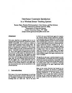
over agents. We believe that a distributed maximal CSP can provide a useful partial solution to an over-constrained distributed CSP, but in some application problems we may want to get completely different partial solutions. Thus, we are going to introduce another subclass of a distributed partial CSP, a distributed hierarchical CSP. In a distributed hierarchical CSP, we assume that each constraint is labeled a positive integer called importance value, which represents an importance of the constraint, and a constraint with a larger importance value is considered more important. We believe this assumption is quite reasonable because a constraint in the real world has some semantics that allows us to introduce such an importance of the constraint. Agents in a distributed hierarchical CSP try to find variable values that minimize the maximum importance value of violated constraints over agents. We believe this type of partial solution is useful because it would be a reasonable compromise when each agent tries to satisfy as many (its own) constraints with large importance values as possible. To put it formally, solving a distributed hierarchical CSP corresponds to finding an optimal solution to the distributed partial CSP specialized by the following. • For each agent i, P Si is made up of {Pi0 , Pi1 , Pi2, . . .}, where Piα is a CSP that is obtained from the original CSP Pi by removing every constraint with an importance value of α or less. • For each agent i, a distance di between Pi and Piα is defined as α. • A global distance is measured as maxi∈A di . Figure 1 shows a distributed 2-coloring problem to illustrate a distributed hierarchical CSP. A node represents a variable and an agent that has the variable. An edge represents constraints, which mean the two connected nodes must be painted in different colors (black or white)2 . An agent knows only the constraints that are relevant to its variable. For example, agent 2 knows only {a, b, e, f}. Assuming the importance value of each constraint given by the number in parentheses3 , a partial CSP of agent 2, for example, is: • P2 : a variable {2} and constraints {a, b, e, f}; • P S2 : a set of the following CSPs: – P20 : P2 , 2 An edge actually represents two constraints (nogoods), which prohibit (black, black) or (white, white) for those connected nodes, respectively. 3 Namely, in this example, we assume that two nogoods for an edge has the same importance value. That doesn’t mean we eliminate the possibility of defining different importance values for these two nogoods.

1

c(3)

4

d(1) h(2)

a(2) e(3)

5

2

b(3)

f(1) i(3)

3

g(3) 6

Figure 1. Distributed 2-coloring problem – P21 : a variable {2} and constraints {a, b, e}, – P22 : a variable {2} and constraints {b, e}, – P23 : a variable {2} and no constraint; • M2 (P2 , P2α ) = α, (α = 0, 1, 2, 3). This example doesn’t have a solution for a global distance of zero. It does, however, have a solution for a global distance of one since a solvable distributed CSP is obtained if agents remove the constraints d and f, which have one as their importance values. Thus, the optimal global distance of this example is one.

5. Algorithms We are going to develop new algorithms for solving a distributed hierarchical CSP by using our previous distributed constraint satisfaction algorithms. The basic idea is very simple. We divide a search process into two parts, i.e., the value space search and the problem space search. In the value space search, agents try to find a solution to some distributed CSP. We will use distributed constraint satisfaction algorithms for the value space search. On the other hand, in the problem space search, agents try to find a solvable distributed CSP from their distributed problem spaces. We will present some heuristic methods for the problem space search. Our new algorithms are based on possible combinations of the value space search and the problem space search.

5.1. Distributed Constraint Satisfaction Algorithm A simple way of realizing the value space search is to use one of our previous distributed constraint satisfaction algorithms, such as the asynchronous backtracking algorithm [12, 13], the asynchronous weak-commitment search algorithm [11, 13] or the distributed breakout algorithm [14]. 5.1.1 Asynchronous Backtracking Algorithm The asynchronous backtracking algorithm (ABT) is basically designed for a distributed CSP where each agent has

one variable. In this algorithm, a priority value is defined for each agent, and each agent changes its variable value asynchronously and concurrently while sending its local information via ok? messages and nogood messages. An agent sends ok? messages to announce its current variable value to other agents. When receiving an ok? message, an agent tries to find a value to its variable that is consistent with higher priority agents. If such a consistent value is found, the agent changes its variable value and sends the new value to neighbors (a set of agents who share constraints) via ok? messages. If such a consistent value is not found, the agent creates a nogood (a set of variable values of higher priority agents) and sends the nogood to the relevant agent via a nogood message. A nogood is a new constraint under which some agent cannot find a consistent variable value. When receiving a nogood message, an agent records the received nogood as a new constraint and tries to satisfy it hereafter. By recording all nogoods, ABT is guaranteed to be complete, i.e., it finds a solution if one exists or terminates if none exists. One drawback of ABT is that a high priority agent tends to have a strong commitment to its variable value. Therefore, if a high priority agent selects a wrong value to its variable, lower priority agents have to perform exhaustive search to revise that wrong value. 5.1.2 Asynchronous Weak-commitment Search Algorithm The asynchronous weak-commitment search algorithm (AWC) is an enhancement of ABT, where agents change their priority values dynamically so that high priority agents do not have strong commitments to wrong variable values. In AWC, an agent uses ok? and nogood messages and follows a similar procedure to that of ABT when receiving those messages. A major difference is that when receiving an ok? message, if an agent cannot find a value to its variable that is consistent with variable values of higher priority agents, the agent not only creates and sends a nogood, but also increases its priority value to make it maximum among neighbors. By increasing a priority value in this way, a wrong variable value of a high priority agent can be revised without performing exhaustive search by lower priority agents. AWC is efficient and guaranteed to be complete by recording all nogoods. However, it suffers from a nogood explosion, i.e., the number of nogoods grows rapidly and thus its checking cost can be very expensive. ABT clearly has the same drawback as well, but such an explosion can be more serious in AWC because an agent in AWC may create nogoods for all neighbors; an agent in ABT, on the other hand, only creates nogoods for higher priority agents. ABT and AWC cannot detect the fact that every agent

reaches the state where all constraints are satisfied. We thus need to incorporate some procedure for its detection into these algorithms. For that purpose, a simple snapshot algorithm like that in [1] should be invoked at certain intervals. 5.1.3 Distributed Breakout Algorithm The distributed breakout algorithm (DB) is a concurrent hill-climbing algorithm incorporated with the breakout method [8] for solving a distributed CSP where each agent has one variable. In DB, a weight is defined for each constraint, and for each value to a variable its evaluation is measured as the summation of the weights of violated constraints. An agent in DB uses ok? and improve messages. An ok? message is used to send a current variable value, and an improve message is used to send possible improvement in the evaluation of variable value. When receiving ok? messages from all neighbors, an agent calculates the evaluation of the current variable value and its possible maximal improvement and sends them to neighbors via improve messages. When receiving improve messages from all neighbors, an agent compares each of their possible maximal improvements with its own one. If one of their improvements is greater than its own one, the agent will skip taking an action and stay unchanged. If its own improvement is the greatest among them, the agent will take an action: changing its variable value if that can reduce its current evaluation or increasing weights of violated constraints if any change of variable value cannot reduce its current evaluation. Note that ties in improvement comparison are broken deterministically by comparing agent identifiers. According to our experimental evaluation, DB is very efficient especially for critically hard instances with solutions [14]. However, it is not a complete algorithm, that is, it may fail to find a solution even if one exists, and it never finds the fact that there is no solution.

5.2. Distributed Hierarchical Constraint Satisfaction Algorithm In a distributed hierarchical CSP, every agent’s problem space has a total order in terms of the degree of relaxation. In this paper, we are going to utilize the total order on a problem space and present two heuristic methods for the problem space search. Both are very simple. One is the method where an agent tries CSPs in its problem space from the most restricted one to the most relaxed one (the removing scheme), and the other is the method where an agent tries vice versa (the adding scheme). With those techniques for the value space search and the problem space search, we will combine those techniques as follows: • ABT from restricted to relaxed (ABT/rm)

• ABT from relaxed to restricted (ABT/ad)

5.2.4 DB/ad

• AWC from restricted to relaxed (AWC/rm)

DB/ad repeatedly applies DB from the maximal level to zero. However, unlike the other algorithms, DB/ad is not complete, that is, it may fail to find an optimal solution to a distributed hierarchical CSP because DB may fail to find a solution to a distributed CSP at a certain level. Note that DB/rm, DB from restricted to relaxed, is not feasible because DB is unable to identify an insoluble distributed CSP that could be used as a chance to relax the problem.

• AWC from relaxed to restricted (AWC/ad) • DB from relaxed to restricted (DB/ad) Before going into the details of these algorithms, we first define a distributed CSP at level α as a distributed CSP that consists of CSPs with distance α. Such a problem can be obtained by making each agent choose a CSP with a distance α (a CSP with every constraint with an importance value of α or less removed) from its problem space. 5.2.1 ABT/rm ABT/rm is the same as the constraint-relaxation method in [10]. As with this method, ABT/rm applies ABT to each level of a distributed CSP in the order from the level zero, an original distributed CSP, to the maximal level. More specifically, ABT/rm repeats the following: from level α = 0 to the maximal level, a) run ABT for a distributed CSP at level α; b.1) if there is no solution to the problem, move to level α + 1 (i.e., relaxing the problem); or b.2) if there is a solution, report the current distributed CSP and its consistent set of variable values as an optimal solution to the distributed hierarchical CSP, and then terminate. Since ABT/rm relaxes a problem by removing constraints, some nogoods created at the previous levels may become obsolete. To remove such an obsolete nogood, we must keep constraints that originate a created nogood and remove the nogood if one of the constraints is removed at the problem relaxation. 5.2.2 ABT/ad While ABT/rm searches a problem space from restricted one to relaxed one, ABT/ad takes the opposite strategy. It repeats: from level α = the maximal level to zero, a) run ABT for a distributed CSP at level α; b.1) if there is a solution, record it and move to level α − 1 (i.e., restricting the problem); or b.2) if there is no solution, report the solution of the previous level as an optimal solution to the distributed hierarchical CSP, and then terminate. Since ABT/ad gradually restricts a problem by adding constraints, nogoods created at the previous levels are all valid throughout the algorithm execution. Thus, we do not need to attach originating constraints to each nogood. 5.2.3 AWC/rm and AWC/ad AWC/rm and ABT/rm are essentially the same. A difference is that we use AWC instead of ABT in AWC/rm. The same is true for the relationship between ABT/ad and AWC/ad.

6. Evaluation We evaluated the performance of these algorithms through experiments on distributed 3-coloring problems. In these experiments, a distributed 3-coloring problem was obtained by generating a 3-coloring problem with m edges (3m constraints/nogoods) and n nodes (n variables) and distributing them so that each agent has one node and the edges that are connected to the node. The algorithms were implemented on a simulator of synchronous distributed system, a typical model of distributed system, on which every agent synchronously performs the following cycle. 1. Receive all the messages which were sent toward the agent at the previous cycle. 2. Perform local computation to change its internal state and determine the contents of messages, and send those messages to other agents. Note that at first cycle an agent does not receive any messages, but it does perform local computation and send messages to other agents. Using this simulator, we evaluated the performance of algorithms in terms of cycles.

6.1. Experiment on Small-sized Instances We first made an experiment on small-sized instances to measure cycles that complete algorithms (ABT/rm, ABT/ad, AWC/rm, AWC/ad) consume until they find an optimal solution. We used four classes of distributed 3coloring problems: problems with 348 edges and 30 nodes, 174 edges and 30 nodes, 87 edges and 30 nodes, and 65 edges and 30 nodes, and randomly generated 10 instances for each class. We chose these classes based on the result of our preliminary experiment to locate an optimal global distance. In generating an instance, we first built a spanning tree and randomly added edges to the tree to ensure graph connectivity, and a random integer with a uniform distribution of 1 to 10 was assigned to each edge as its importance

algorithm ABT/rm ABT/ad AWC/rm AWC/ad

348 edges 30 nodes % cycle 0 − 0 − 100 1646.7 100 462.8




Table 1. Average cycle to find an optimal solution.

• ABT/rm (the constraint-relaxation method in [10]) and ABT/ad perform very poorly for all instances. This is due to inefficiency of ABT as the value space search. • AWC/rm is more expensive than AWC/ad. This is because AWC generally works poorly in detecting an insoluble problem due to its poor ability in nogood handling. AWC/rm continues to deal with such insoluble problems until it finds an optimal solution, and thus its performance deteriorates. • For problems with 65 edges and 30 nodes, the difference between AWC/rm and AWC/ad is not so large in terms of average cycles. This is because for some instance with a low optimal global distance, AWC/rm can be better because it starts from the original distributed CSP toward the relaxed ones and thus finding an optimal solution with such a low optimal global distance very easily. Figure 2 shows typical anytime curves for AWC/ad for an instance of problems with 65 edges and 30 nodes. An anytime curve illustrates how a global distance of the best solution found so far is improved as time proceeds. A curve in figure 2 is averaged over 10 trials. Note that the removing 4 Three constraints/nogoods corresponding to one edge have the same importance value in this experiment.

AWC/ad 12 10 global distance

value4 . By this method, an optimal global distance lies on 8–9 for problems with 348 edges and 30 nodes, 6–8 for problems with 174 edges and 30 nodes, 2–5 for problems with 87 edges and 30 nodes, and 0–2 for problems with 65 edges and 30 nodes. For each instance, a complete algorithm made 10 trials with randomly generated different sets of initial variable values. We set the bound for cycles at 10000 and terminated a trial if an algorithm fails to find an optimal solution within the bound. Such a trial is counted as 10000 cycles. Table 1 shows for 100 trials (10 instances with 10 trials) of each class of problems, the cycles consumed until each algorithm finds an optimal solution (averaged over 100 trials) and the percentage of times each algorithm completed within the bound. These results indicate:

8 6 4 2 0 0

500

1000

1500 Cycle

2000

2500

3000

Figure 2. Anytime curve for an instance of problems with 65 edges and 30 nodes (averaged over 10 trials).

scheme algorithm, such as ABT/rm or AWC/rm, cannot obtain any solution until it finds an optimal solution because it starts from a tight and usually insoluble distributed CSP. However, the adding scheme algorithm proceeds while getting a series of non-optimal solutions and thus being able to produce a nearly-optimal solution while searching for an optimal solution.

6.2. Experiment on Large-sized Instances For large-sized instances, the performance of the above algorithms becomes very poor since each of these searches for an optimal solution. It seems reasonable to assume that we should aim at a nearly optimal solution in place of an optimal solution. Accordingly, the anytime characteristics may be important. As we showed in the experiment on small-sized instances, the removing scheme is not appropriate in terms of the anytime characteristics, and thus we used only the promising adding scheme, AWC/ad and DB/ad, to compare their performance. In this experiment, we didn’t use nogood recording in AWC/ad. Generally speaking, nogood recording can be computationally expensive especially for large-sized instances. Fortunately, without nogood recording, AWC has

algorithm

AWC/ad DB/ad

180 + 243 edges 90 nodes % cycle 100 121.5 100 235.6




Table 2. Average cycle to find a solution to the problem at the level 6. the way to break deadends, i.e., changing priorities among agents, and is able to find a solution to a solvable distributed CSP in many cases. This means that, without nogood recording, AWC/ad is feasible even if it loses its completeness. We made an experiment on distributed 3-coloring problems with m = 2n + 2.7n and m = 2.7n + 2.7n (m: the number of edges, n: the number of nodes). The former includes difficult instances for DB, and the latter does for AWC [14]. The values of n are 90 and 120 in this experiment. An instance was generated such that, for each n, 1. create 2n or 2.7n edges by the method described in [7] (that produces a solvable and connected graph), each of which is labeled by a random integer with a uniform distribution of 6 to 10. 2. add 2.7n edges randomly, each of which is labeled by a random integer with a uniform distribution of 1 to 5. This method ensures that every distributed CSP at more than the 5 level has consistent variable values, and thus an optimal distance is located at not more than the 5 level. It also ensures that there is a hard solvable distributed CSP between the levels 6 and 10. Thus, the adding scheme definitely confronts some hard instance on the way from the maximal level to the optimal level. We evaluated the performance of algorithms by how quickly they go through those hard and solvable levels. Table 2 shows the cycles consumed until each algorithm finds a solution to a distributed CSP at the level 6 after starting with the one at the level 10 (averaged over 100 trials (10 instances with 10 trials)). Each trial started with randomly chosen initial variable values and was terminated if it fails to find a solution to the problem at the level 6 within 50000 cycles. This table also shows the percentage of times the algorithm was successfully completed. From these results, we can see the following: • DB/ad is effective for problems with 324 + 324 edges and 120 nodes while AWC/ad is effective for other problems. We suppose that this is due to the properties of AWC and DB. DB is more efficient than AWC for solvable instances of m = 2.7n (especially when n is large); on the other hand, AWC is more efficient

than DB for those of m = 2n. Thus, DB/ad can move more quickly among these levels of distributed CSPs (the level 10 to 6) while it efficiently finds a solution at a certain level of problem for 324 + 324 edges and 120 nodes; on the other hand, AWC/ad can do for 180 + 243 edges and 90 nodes and 240 + 324 edges and 120 nodes. • In spite of no guarantee of finding a solution to the problem at the level 6, most instances are successfully completed by AWC/ad and DB/ad. On the other hand, ABT/ad (not in table 2) does have such guarantee, but more cycles are consumed than AWC/ad or DB/ad. Furthermore, both ABT/ad and AWC/ad combined with nogood recording are computationally expensive because they need to check all recorded nogoods.

7. Conclusion We showed a distributed hierarchical CSP to give another partial solution to an over-constrained distributed CSP and presented a series of new algorithms for solving a distributed hierarchical CSP. We believe this class of problem would be important since a real-life problem in MAS may be easily overconstrained when each of multiple users delegates an agent to satisfy his/her constraints. A partial solution provided by a distributed hierarchical CSP is one promising solution for the situation. Algorithms presented in this paper are combinations of our previous distributed constraint satisfaction algorithms and the simple problem space search methods. One may feel that these algorithms are so straightforward that they would need more sophisticated techniques especially for the problem space search. However, we believe the problem space search should be simple because the search cost in a problem space is very high. Finally, we point out the current limitation of our algorithms. All the algorithms in this paper are for an overconstrained distributed CSP where each agent has one variable because we use distributed constraint satisfaction algorithms designed for such a problem as the value space search. However, by using the algorithm presented in [15]

as the value space search, we can easily extend our algorithms to the problem where each agent has multiple local variables. Our future work will include evaluating the performance of those extended algorithms.

References [1] K. Chandy and L. Lamport. Distributed snapshots: Determining global states of distributed systems. ACM Transaction on Computer Systems, 3(1):63–75, 1985. [2] S. E. Conry, K. Kuwabara, V. R. Lesser, and R. A. Meyer. Multistage negotiation for distributed constraint satisfaction. IEEE Transactions on Systems, Man and Cybernetics, 21(6):1462–1477, 1991. [3] E. C. Freuder and R. J. Wallace. Partial constraint satisfaction. Artificial Intelligence, 58(1–3):21–70, 1992. [4] K. Hirayama and M. Yokoo. Distributed partial constraint satisfaction problem. In G. Smolka, editor, Principles and Practice of Constraint Programming –CP97, volume 1330 of Lecture Notes in Computer Science, pages 222–236. Springer-Verlag, 1997. [5] M. N. Huhns and D. M. Bridgeland. Multiagent truth maintenance. IEEE Transactions on Systems, Man and Cybernetics, 21(6):1437–1445, 1991. [6] V. R. Lesser and D. D. Corkill. The distributed vehicle monitoring testbed: A tool for investigating distributed problem solving networks. AI Magazine, 4(3):15–33, 1983. [7] S. Minton, M. D. Johnston, A. B. Philips, and P. Laird. Minimizing conflicts: a heuristic repair method for constraint satisfaction and scheduling problems. Artificial Intelligence, 58(1–3):161–205, 1992. [8] P. Morris. The breakout method for escaping from local minima. In Proceedings of the Eleventh National Conference on Artificial Intelligence, pages 40–45, 1993. [9] K. P. Sycara, S. Roth, N. Sadeh, and M. Fox. Distributed constrained heuristic search. IEEE Transactions on Systems, Man and Cybernetics, 21(6):1446–1461, 1991. [10] M. Yokoo. Constraint relaxation in distributed constraint satisfaction problem. In 5th International Conference on Tools with Artificial Intelligence, pages 56–63, 1993. [11] M. Yokoo. Asynchronous weak-commitment search for solving distributed constraint satisfaction problems. In Principles and Practice of Constraint Programming –CP95, volume 976 of Lecture Notes in Computer Science, pages 88– 102. Springer-Verlag, 1995. [12] M. Yokoo, E. H. Durfee, T. Ishida, and K. Kuwabara. Distributed constraint satisfaction for formalizing distributed problem solving. In Proceedings of the 12th IEEE International Conference on Distributed Computing Systems, pages 614–621, 1992. [13] M. Yokoo, E. H. Durfee, T. Ishida, and K. Kuwabara. The distributed constraint satisfaction problem: formalization and algorithms. IEEE Transactions on Knowledge and Data Engineering, 10(5):673–685, 1998. [14] M. Yokoo and K. Hirayama. Distributed breakout algorithm for solving distributed constraint satisfaction problems. In Proceedings of the Second International Conference on Multi-Agent Systems, pages 401–408, 1996.

[15] M. Yokoo and K. Hirayama. Distributed constraint satisfaction algorithm for complex local problems. In Proceedings of the Third International Conference on Multi-Agent Systems, pages 372–379, 1998.