Noname manuscript No. (will be inserted by the editor)
Distributed Genetic Programming on GPUs using CUDA
Simon Harding · Wolfgang Banzhaf
Received: date / Accepted: date
Abstract Using of a cluster of Graphics Processing Unit (GPU) equipped computers, it is possible to accelerate the evaluation of individuals in Genetic Programming. Program compilation, fitness case data and fitness execution are spread over the cluster of computers, allowing for the efficient processing of very large datasets. Here, the implementation is demonstrated on datasets containing over 10 million rows and several hundred megabytes in size. Populations of candidate individuals are compiled into NVidia CUDA programs and executed on a set of client computers - each with a different subset of the dataset. The paper discusses the implementation of the system and acts as a tutorial for other researchers experimenting with genetic programming and GPUs. Simon Harding Department of Computer Science, Memorial University Canada E-mail:
[email protected] Wolfgang Banzhaf Department of Computer Science, Memorial University Canada E-mail:
[email protected]
2
Keywords Genetic Programming · GPU · CUDA
1 Introduction
Graphics Processing Units (GPUs) are fast, highly parallel processor units. In addition to processing 3D graphics, modern GPUs can be programmed for more general purpose computation. The GPU consists of a large number of ‘shader processors’, and conceptually operates as a Single Instruction Multiple Data (SIMD) or Multiple Instruction Multiple Data (MIMD) stream processor. A modern GPU can have several hundred of these stream processors, which combined with their relatively low cost, makes them an attractive platform for scientific computing.
1
Implementations of Genetic Programming (GP) on Graphics Processing Units (GPUs) have largely fallen into two distinct evaluation methodologies: population parallel or fitness case parallel. Both methods exploit the highly parallel architecture of the GPU. In the fitness case parallel approach, all the fitness cases are executed in parallel with only one individual being evaluated at a time. This can be considered a SIMD approach. In the population parallel approach, multiple individuals are evaluated simultaneously. Both approaches have problems that impact performance. The fitness case parallel approach requires that a different program is uploaded to the GPU for each evaluation. This introduces a large overhead. The programs need to be compiled (CPU side) and then loaded into the graphics card before any evaluation can occur. Previous work has shown that for smaller numbers of fitness cases (typically less than 1000), this overhead is larger than the increase in computational speed [1, 4, 7]. In these use cases there is no benefit to executing the program on the GPU. For some 1
The web site www.gpgpu.org is a useful starting point for GPU programming information.
3
problems, there are fewer fitness cases than shader processors. In this scenario, some of the processors are idle. This problem will become worse as the number of shader processors increases with new GPU designs. Unfortunately, a large number of classic benchmark GP problems fit into this category. However, there are problems such as image processing that naturally provide large numbers of fitness cases (as each pixel can be considered as different fitness case) [3, 5].
GPUs are considered as SIMD processors (or MIMD when the processors can handle multiple copies of the same program running with different program counters [12]). When evaluating a population of programs in parallel, the common approach so far is to implement some form of interpreter on the GPU [12, 10, 15]. The interpreter is able to execute the evolved programs (typically machine code like programs represented as textures) in a pseudo-parallel manner. To see why this execution is pseduo-parallel, the implementation of the interpreter needs to be considered.
A population can be represented as a 2D array, with individuals represented in the columns and their instructions in the rows. The interpreter consists of a set of IF statements, where each condition corresponds to a given operator in the GP function set. The interpreter looks at the current instruction of each individual, and sees if it matches the current IF statement condition. If it does, that instruction is executed. This is happening for each individual in the population in parallel, and for some individuals the current instruction may not match the current IF statement. These individuals must wait until the interpreter is reaches their instruction type. Hence, for this approach some of the GPU processors are not doing useful computation. If there are 4 functions in the function set, we can expect that on average at least 3/4 of the shader processors are ‘idle’. If the function set is larger, then more shaders will be ‘idle’.
4
Despite this idling, population parallel approaches can still be considerably faster than CPU implementations.
The performance of population parallel implementations is therefore impacted by the size of the function set used. Conversely, the fitness case parallel approaches that are impacted by the number of fitness cases. Population parallel approaches are also largely unsuited for GPU implementation when small population sizes are required.
In this paper, we present a data parallel approach to GP where we attempt to mitigate the overhead of program compilation. Using multiple computers, we are able to execute complex, evolved programs and efficiently process very large datasets.
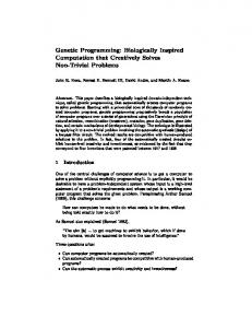
Fig. 1 Algorithm overview. The root computer administers the client computers. The root is responsible for maintaining the population and distributing sections of the dataset to the GPU equipped client computers. Client computers can be capable of executing programs (i.e. contain a compatible GPU) and/or be capable of compiling CUDA programs using NVCC. Different combinations of compiling and executing computers can be used, depending on the resources available.
5
2 Design Considerations
One of the purposes of this investigation was to determine if it is possible to utilize the spare processing capabilities of computers in a student laboratory. As the resources are shared, the number of available machines and available processing power is inconsistent. In this work, results are typically obtained using between 14 and 16 computers.
The computers used here contain very low end video cards: the NVidia GeForce 8200. Each 8200 GPU has 8 stream processors and access to 128Mb of RAM. As the processor is shared with the operating system, the free GPU memory on each machine is approximately 80Mb. According to Wiki [14], the expected speed of these cards is 19 giga floating point operations per second (Gigaflops). By comparison, a high end GPU like the GeForce GTX 295 has 480 stream processors providing 1,788 Gigaflops.
As the laboratory is not a dedicated cluster, other design requirements needed to be considered. These include ensuring the file server and network utilization were kept to a minimum.
Although currently the GPUs in this setup are low end, we are confident that the approach detailed here will also be applicable to high-end and future devices.
The root computer node used here is equipped with an Intel Q6700 quad-core, 4Gb of RAM and Windows XP. The client computers used Gentoo Linux, AMD 4850e processors and 2Gb of RAM. The software can work on any combination of Linux and Windows platforms.
6
3 Algorithm Overview
The algorithm devised here is an implementation of a parallel evolutionary algorithm, where there is a master controller (called the ‘root’) and a number of slave computers (or ‘clients’), as shown in figure 1. In summary the algorithm works in the following manner:
1. Process is loaded onto all computers in the cluster.
2. Root process is started on the master computer.
3. Each computer announces its presence using a series of short UDP broadcasts. The root listens to these broadcasts and compiles a list of available machines.
4. After announcing their presence, each of the client machines starts a server process to listen for commands from the root.
5. After 2 minutes, the root stops listening for broadcasts and connects to to each client machine.
6. Upon connecting to each machine, each client is asked what their capabilities are (in terms of CUDA compiler and device capability).
7. The root distributes sections of the fitness set to each CUDA capable computer.
7
8. The root initializes the first population.
9. Root begins the evolutionary loop.
(a) Convert population to CUDA C code.
(b) Parallel compile population.
(c) Collate compiled code and resend to all compiling clients.
(d) Perform execution of individuals on all GPU equipped clients.
(e) Collect (partial) fitness values for individuals from GPU equipped clients.
(f) Generate next population, return to step 9a.
The following sections describe the implementation details of each step.
4 Cartesian Genetic Programming
The genetic programming system used is a version of CGP[11], and is largely the same implemented as used in our previous GPU work [7, 4, 5]. CGP uses a genotype-phenotype mapping that does not require all of the nodes to be connected to each other, resulting in a bounded variable length phenotype. Each node in the directed graph represents a particular function and is encoded by a number
8
of genes. The first gene encodes the function the node is representing, and the remaining genes encode the location where the node takes its inputs from, plus one parameter that is used as a constant. Hence each node is specified by 4 genes. The genes that specify the connections do so in a relative form, where the gene specifies how many nodes back to connect [8]. Special function types are used to encode the available inputs. Details can be found in [6]. The graph is executed by recursion, starting from the output nodes down through the functions, to the input nodes. In this way, nodes that are unconnected are not processed and do not effect the behavior of the graph at that stage. For efficiency, nodes are only evaluated once with the result cached, even if they are connected to multiple times. The function set was limited to input, addition, subtraction, multiplication and division.
5 C], Mono and Communication
Mono is an open source implementation of Microsoft’s .net platform. Mono is available for many different operating systems. The platform is based around a virtual machine and a large number of libraries. Microsoft call the virtual machine a ‘common language runtime’ (CLR). Code from many languages can be compiled to the byte-code used on the CLR. Here, the C] language is used. The main reason for using C] is that much of our previous work has been developed using these tools, notably our other GPU work using Microsft Accelerator [7, 4].
9
In this implementation, we use a method of inter-process communication called Remoting. Remoting allows for objects to communicate to other objects running in other applications - including applications running on different machines. Using C] and the .Net framework, remoting can be a straightforward task. In essence, it allows for objects to be instantiated on a remote machine, and the methods executed on that remote object with the results visible locally. The process can be made virtually transparent, with the only additional code needed to provide an object server and code to attach to such a server. Almost any object can be used with the remoting framework.
Network communication performance was increased by using compression where applicable. When transferring data arrays, it was found that in memory GZip compression worked very well. For example, when transferring the compiled programs to each of the clients, the data compression was often 10:1 with a compression time of less than 0.05 seconds. This reduced the network traffic by the same ratio.
Remote objects are compatible across different platform types. Development was performed using Microsoft Visual Studio under Windows. Testing was done using Windows computers with the final deployment to Linux.
On the root computer, running Microsoft Windows, the Microsoft CLR was used. Mono’s (version 2.2) garbage collector contains several known bugs, and the program would crash when too much memory was allocated. Switching to the Microsoft CLR solved this problem. Mono was adequate on the client computers, as they did not perform so much memory intensive work (such as maintaining the population, handling results and code generation).
10
6 Interfacing C] to CUDA
CUDA is an extension to the C programming language, and programs written with CUDA are typically written as pure C programs. However, many libraries exist that expose the programming interface of the CUDA driver to other programming environments. In this work, the CUDA.net library from GASS is used [2]. This library allows any .net language to communicate with the CUDA driver. There are similar libraries available for other languages e.g. jacuzzi and jCUDA for Java. Accessing the CUDA driver allows applications to access the GPU memory, load code libraries (modules) and execute functions. The libraries themselves still need to be implemented in C and compiled using the CUDA nvcc compiler.
7 Compilation
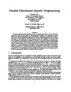
To mitigate the slow compilation step in the algorithm, a parallelized method was employed. Figure 2 shows how the compilation speed varies with the number of individuals in a population. The compilation time here includes rendering the genotypes to CUDA C code, saving the code and running the compiler. For a single machine, the compilation time increases linearly with the size of the population. For large populations, the compilation phase quickly becomes a significant bottleneck. Using distributed compilation, for typical population sizes, it is possible to maintain a rapid compilation phase.
11
Fig. 2 How compilation speed varies with the number of individuals in a population, comparing single machine complilation to that using 14 machines within the cluster.
7.1 CUDA’s module files
CUDA allows for library files called ‘modules’ to be loaded into the GPU. Modules are libraries of functions that can be loaded, executed on the GPU and then unloaded. As shown in figure 3, module load times increase linearly with the number of functions (or individuals) they contain. However, there is a constant overhead to this, unloading the module, transferring the module across the network and other file handling operations. Therefore it is preferable to minimize the number of module files that are created. To compile a module, the user first creates a source file containing only CUDA functions, these should be declared as in the following example:
extern "C" __global__ void Individual0(
12
Fig. 3 Module loading times for various sized populations (and hence number of functions in a .cubin library).
float* ffOutput, float* ffInput0, int width, int height) When compiled, each of those functions is exposed as a function in the compiled library. The compiler was executed with the command line: nvcc modulename.cu --cubin Modules have the file extension ‘.cubin’. Internally, the .cubin files are text files with a short header, followed by a set of code blocks representing the functions. The code blocks contain the binary code for the compiled function in addition to information about memory and register usage.
13
7.2 Parallel compilation of CUDA modules
It is possible to merge the contents of module files together by simply appending .cubin files together. This allows u to compile sections of a library independently of each other and then reduce these sections into a single module. However, only one header is permitted per .cubin file. In this implementation, the following process is used to convert the genotypes into executable code.
1. Convert the population to CUDA. This process is performed on the root machine. At this stage, the population is divided up into sections - equal to the number of machines available for compilation. Each section is then converted to CUDA using the code generator described in section 9. This stage is performed in parallel across the cores on the root computer, whereby a separate thread is launched for each section of the population’s code generator.
2. Send the uncompiled code to the distributed machines. In parallel, each section of uncompiled code is transmitted to a computer for compilation. The remote computer saves the code to the local disk, before compilation. The remote computer then loads the .cubin file from disc and returns it to the root computer.
3. The host computer merges the returned .cubin files together (in memory) and then sends the merged version back to all the computers in the grid for execution. Again, this happens in parallel with remote computers sending back their compiled files asynchronously.
14
Graph length Population Size 256
512
1024
2048
4096
32
3.87
3.95
3.63
4.84
5.71
64
4.33
4.75
3.66
4.67
4.31
128
4.64
5.04
5.64
6.09
5.18
256
5.95
5.32
5.05
6.59
4.47
512
5.56
6.54
5.52
4.68
7.36
1024
8.89
6.72
7.09
10.94
6.86
2048
13.99
12.55
14.61
12.75
12.88
4096
16.90
18.43
17.57
17.55
-
Table 1 Times (in seconds) to perform the entire compilation process using the parallel compilation method. Due to the memory allocation issues, some results are incomplete.
Figure 2 shows the performance benefit in this parallel compilation method. For typical population sizes, the parallel compilation means that each processor is only compiling a small number of functions - and for this type of size the compiler is acting at its most efficient ratio of compilation time to function count. However, it should be noted that the compilation time does not appear to scale linearly with the number of compiling clients. Tables 1 and 2 show the average times taken to compile various sized populations, with various sized program lengths. The results show a clear performance increase using the parallel compilation method. Note that for these results (and other related results reported here) there are missing values for the largest population/graph length. This is due to a limitation in the 32-bit version of .Net where very large objects (>1.5Gb) cannot be allocated. Table 3 shows the average time taken to send the compiled code to all the client computers. This also includes the time taken to load the CUDA module into memory.
15
Graph length Population Size 256
512
1024
2048
4096
32
1.22
1.22
1.22
1.22
1.30
64
1.55
1.55
1.54
1.54
1.54
128
2.20
2.20
2.21
2.18
2.20
256
3.54
3.73
3.60
3.55
3.61
512
6.43
6.44
6.43
6.45
6.47
1024
13.33
13.56
13.43
13.45
13.41
2048
36.16
36.26
36.06
36.01
36.16
4096
129.43
130.74
129.91
129.58
-
Table 2 Times (in seconds) to perform the entire compilation process using a single threaded compilation method. Due to the memory allocation issues, some results are incomplete.
Graph length Population Size 256
512
1024
2048
4096
32
2.40
3.28
2.17
3.16
4.26
64
4.66
5.33
2.91
3.53
3.90
128
2.70
3.67
4.00
3.53
2.73
256
1.81
2.40
1.65
2.13
1.59
512
2.02
1.56
1.78
1.46
2.05
1024
2.06
3.98
2.03
3.30
2.21
2048
3.15
3.20
3.38
3.50
2.88
4096
4.75
5.18
6.53
5.67
-
Table 3 Average times (in seconds) to distribute compiled populations to the clients in the cluster. Due to the memory allocation issues, some results are incomplete.
8 Code generation
Code generation is the process of converting the genotypes in the population to CUDA compatible code. During development, a number of issues were found that made this
16
process more complicated than expected. One issue was that the CUDA compiler does not like long expressions. In initial tests, the evolved programs were written as a single expression. However, when the length of the expression was increased the compilation time increased dramatically. This is presumably because they are difficult to optimize.
Another issue is that functions with many input variables will cause the compilation to fail, with the compiler complaining that it had been unable to allocated sufficient registers. In initial development, we had passed all the inputs in the training set to each individual - regardless of if the expression used them. This worked well for small numbers of inputs, however the training set that was used to test the system contains 41 columns. The solution to this problem was to pass the function only the inputs that it used. However, this requires each function to be executed with a different parameter configuration. Conveniently, the CUDA.Net interface does allow this, as the function call can be generated dynamically at run time. The other issue here is that all/many inputs may be needed to solve a problem. It is hoped that this is a compiler bug and that it will be resolved in future updates to CUDA.
The conversion process is also amenable to parallel processing, as different individuals can be processed in isolation from each other. The conversion time from individual to CUDA code is very fast (see table 4), so it did not seem necessary to use the remote clients for this stage. Instead, the process is started as a number of threads on a multi-core computer. With the number of individuals being processed by each thread equal to the total population size divided by the number of compilation clients.
17
Graph length Population Size 256
512
1024
2048
4096
32
0.002
0.068
0.008
0.004
0.005
64
0.104
0.005
0.025
0.004
0.035
128
0.004
0.050
0.008
0.034
0.024
256
0.031
0.013
0.034
0.039
0.067
512
0.017
0.042
0.074
0.030
0.077
1024
0.051
0.081
0.105
0.148
0.145
2048
0.117
0.141
0.213
0.128
0.162
4096
0.145
0.252
0.174
0.224
-
Table 4 Times (in seconds) to convert population to CUDA code. Due to the memory allocation issues, some results are incomplete.
9 CUDA C Code Generation
The code in figure 4 illustrates a typical generated individual. As noted before, long expressions failed to compile within a reasonable time. The workaround used here was to limit the number of nodes that made up a single statement, and then used temporary variables to combine these smaller statements together. It is unclear what the best length is for statements, but it is more likely to be a function of how many temporary variables (and hence registers) are used. The names for the temporary variables relate to the node index in the graph that the statement length limit was introduced. The final output of the individual is stored in a temporary variable (r). As this is a binary classification problem, it was convenient to add code here to threshold the actual output value to one of the two classes. During code generation it was also possible to remove redundant code. When parsing a CGP graph recursively, unconnected nodes are automatically ignored so do not
18
Fig. 4 Example of the CUDA code generated for an individual.
need to be processed. It is also possible to detect code which serves no purpose e.g. division where the numerator and denominator are the same, or multiplication by 0. This can be seen as another advantage of pre-compiling programs over simple interpreter based solutions. CGP programs have a fixed length genotype, which is kept constant throughout an experiment. The length of the phenotype program (in operations) is always less than the length of the genotype (in nodes). Table 5 shows the average, total number of operations in a generated module for each graph (genotype) size and population size. The number of operations is very low (typically between 1% and 0.1%) compared to the maximum possible number of operations (population size × genotype length).
19
Graph length Population Size 256
512
1024
2048
32
167
127
134
125
64
224
267
246
259
128
484
509
520
575
256
1002
1026
1070
1046
512
1867
2033
2130
2097
1024
3494
3628
3669
4507
2048
7010
7620
8447
11195
Table 5 Average operations in the generated module. Each module represents all the individuals in the current population.
10 Training Data
To test the implementation, a substantial data set set was required. The fitness set used here is the network intrusion classification data from the KDD Cup 1999 [9]. The data has of 4,898,431 fitness cases. Each case has 42 columns, including a classification type. During preprocessing, each of the descriptive, textual fields in the dataset was encoded numerically. On disc in text format, the entire dataset is approximately 725Mb. This would be too much data for a (typical) single GPU system to manage efficiently, as GPUs tend to have relatively small amounts of memory. It is considerably larger than the 128Mb (with 80Mb memory available) GPUs available on each of the client computers. The training set is split into a number of sets of data - one for each of the client computers. This is done dynamically during the start up phase of the algorithm. When split between 16 client machines, the GPU memory requirement of each subset of data is approximately 46Mb.
20
To improve network efficiency, the data is compressed in memory before sending to each of the clients. This reduced the time taken to transfer data from over 10 minutes to less than 3 minutes. Training data needs to be loaded into the GPU only once. Also, memory for storing the output of the evolved programs and other tasks only needs to be allocated once.
11 Distributing the computation
Each client performs part of the fitness calculation, allowing for very large datasets to be processed efficiently. After compilation, each client is sent a copy of the compiled library (.cubin). The CUDA driver allows for modules to be loaded in by a direct memory transfer - avoiding the use of the disc. As the cubin files are relatively small, the root process can send these to all clients simultaneously without stressing the network. Next, the root instructs the client machines to start executing the individuals on their section of the training set. When this is complete, the root collects fitness information from each individual. The root calculates the total fitness of an individual by summing each partial fitness fitness. For these stages, each client is controlled by an independent thread from the root. Clients may return their results asynchronously. The total compute time is determined by the slowest machine in the cluster. For this demonstration, the entire dataset is used to determine the fitness of an individual. An obvious extension here would be to divide the partial fitnesses into a training and validation set. In previous work on images, scores were collected to be used as both seen and unseen data fitness values [5]. As adding extra fitness cases does
21
not add too much overhead to the process (the compilation phases etc. are likely more time consuming) the approach is very convenient. Another improvement may be to implement a K-fold validation algorithm. Logically, K would be the number of client machines.
12 Fitness Function
For this prototype application, the task was for evolution to classify the network intrusion data set into either valid or invalid packets, with an invalid packet indicating a network intrusion. The fitness function here consisted of calculating the sum of the error between the expected output and the output of the evolved program. Here the output of the evolved program was automatically thresholded to 0 or 1. Hence, the fitness here is the total number of incorrectly classified packets. These calculations (truncation of the program output and summation of the error) were also performed on the GPU, with the partial results collated by the root. The root is responsible for then summing the partial results to provide an overall fitness for each individual.
13 Evaluation performance
Table 6 shows the overall total performance, in Giga GP Operations Per Second, for each of the genotype/population sizes. Peak performance (as shown in table 7) is considerably higher. The number of individuals processed per second varied from 5.8 for the smallest population size, to 86 per second for populations of 2048 individuals. See Figure 5. These numbers are disappointingly low, as each client has a theoretical
22
Graph length Population Size 256
512
1024
2048
32
0.19
0.14
0.16
0.14
64
0.23
0.29
0.29
0.29
128
0.50
0.50
0.54
0.51
256
0.92
0.94
0.99
0.95
512
1.47
1.63
1.66
1.64
1024
1.38
1.47
1.50
1.71
2048
1.59
1.68
1.82
2.25
Table 6 Average Giga GP Operations Per Second.
Graph length Population Size 256
512
1024
2048
32
0.34
0.38
0.33
0.33
64
0.53
0.59
0.53
0.58
128
0.94
0.85
0.93
0.99
256
1.56
1.51
1.58
1.82
512
2.29
2.69
2.36
2.50
1024
2.47
2.89
2.92
3.41
2048
2.41
2.62
2.31
3.44
Table 7 Maximum Giga GP Operations Per Second.
raw processing speed of approximately 19 GFlops. The figure here is much lower as it includes the compilation overhead, data transfer times and the overhead of the total error calculation of the fitness function itself. The GPU was also shared with the operating system, which again is expected to reduce the efficiency.
23
Fig. 5 Average number of individuals processed per second.
14 Image processing
In previous work, we have used MS Accelerator [13] as the GPU API when evolving image filters [5]. Using this approach, substantial speed increases over a CPU implementation were achieved. The fastest speed achieved on a single GPU was a peak of 324 million GP operations per second (MGPOp/s) .
With very little modification, it is also possible to do evolutionary image processing using the framework described in this paper. As with [5] the task was to find a program that would act as a filter, transforming one image into another. The evolved program takes 9 inputs (a pixel and its neighbourhood) and outputs a new value for the centre pixel.
24
The first stage requires the generation of the training data. Using a similar concept to [5], an image was converted into a dataset where each row contained a pixel, its neighbouring 8 pixels and the value of the corresponding target pixel. This allows the problem to be treated as a regression problem. The fitness is the sum of the error between the expected output and the output of the evolved program for all pixels. To test the system implemented here, a large image was used (3872 x 2592 pixels, which is the native resolution of a 10Mega pixel digital camera). The image was converted to gray scale, and then converted to the format described above. The desired output image was an “embossed” version of the input (created using Paint.Net). The dataset contains 10,023,300 rows and 10 columns, which is approximately 400Mb of data in memory. As each row is independent of each other, the image can be split across the client computers in the same way as before. A number of short evolutionary runs of 10 generations were performed for each population size/genotype length pair. From these, an indication of the performance of the system can be obtained.
Graph length Population Size 256
512
1024
2048
32
1.49
0.87
1.16
1.42
64
2.34
2.21
1.81
2.03
128
3.01
2.85
2.65
4.60
256
4.72
4.39
5.44
5.08
512
4.73
5.81
6.37
6.39
1024
5.57
6.10
4.71
6.56
2048
5.77
5.45
5.41
7.06
Table 8 Average Giga GP Operations Per Second when evolving the emboss image filter.
25
Graph length Population Size 256
512
1024
2048
32
2.94
1.89
2.62
1.83
64
4.92
4.21
3.31
3.98
128
5.48
4.23
6.05
7.61
256
5.91
6.86
10.70
10.96
512
6.69
10.42
11.22
11.47
1024
7.25
9.55
6.29
12.74
2048
7.72
8.49
7.61
10.56
Table 9 Peak Giga GP Operations Per Second when evolving the emboss image filter.
Tables 8 and 9 show the average and peak performance when using 16 client computers on this task. The peak results observed in [5], when evolving the same type of filter, the average performance was 129 MGPOp/s and a peak of 254 MGPOp/s. On average, this implementation achieved 4.21 GGPOp/s across all population and graph sizes. Comparing the best, average performance this implementation is approximately 55 times faster than the MS Accelerator implementation operating on a single GPU.
The speed up was likely a combination of both using CUDA (as compared to Accelerator), multiple computers and a larger input image size. On a single GPU, it was found that Accelerator was unable to cope with images larger than 2048 x 2048 pixels. By splitting up the image data, each of the client computers is only required to operate on a much smaller amount of data, which is likely to make the processing more efficient.
26
15 Conclusions and Future Work
We have developed a distributed, GPU based implementation of a GP system. Compared to previous work, this implementation allows for the use of very large datasets and complex programs. Although already a fairly sophisticated implementation, there are a number of additional components we wish to develop. In future we wish to investigate the behavior of this system on a cluster containing more capable GPUs. There does not seem to be any reason why the process described here should not scale to higher end GPUs. Another future experiment is to test the functionality of having a different number of compiling computers to executing computers. In the current configuration, the same computers are used for both compiling the CUDA programs and executing the programs. However, the implementation allows for a different number of compiling clients to ones that actually run the program. It should be possible to improve the compilation speed further by spreading it over other computers. This is particularly appealing, as machines used for compiling CUDA do not have to have CUDA compatible GPUs installed. Other modifications to the software will allow for the use of multiple GPUs in the same computer. Some common video cards, notably the GeForce 9800, have multiple GPUs that can be individually addressed. Presently, we assume only one GPU per client. A further issue we have yet to address is that of fault tolerance. As a shared resource, the computers in the lab are likely not only be used at the same time by
27
students - but may also be turned off during the experiment. Currently, there is no recovery mechanism implemented. As noted previously, the collection of results is limited by the slowest client in the cluster - which may slow down results on a heterogeneous cluster. The CUDA driver allows the controlling application to determine the properties of the hardware, including the available memory, clock speed and number of allowed threads. Using this information, it should be possible to better distribute the processing load across the clients. Machines with higher end GPUs would get more work to do - and therefore would not be idle, waiting for slower clients to finish.
Acknowledgements This work was supported by NSERC under discovery grant RGPIN 283304-07 to WB. The authors also wish to thank NVidia for hardware donations and GASS for technical support with the CUDA.Net toolkit. We also wish to thank WBL for his helpful feedback.
References 1. Chitty, D.M.: A data parallel approach to genetic programming using programmable graphics hardware. In: D. Thierens, H.G. Beyer, et al. (eds.) GECCO ’07: Proceedings of the 9th annual conference on Genetic and evolutionary computation, vol. 2, pp. 1566–1573. ACM Press, London (2007). URL http://doi.acm.org/10.1145/1276958.1277274 2. GASS Ltd.: Cuda.net. http://www.gass-ltd.co.il/en/products/cuda.net/ 3. Harding, S.: Evolution of image filters on graphics processor units using cartesian genetic programming. In: J. Wang (ed.) 2008 IEEE World Congress on Computational Intelligence. IEEE Computational Intelligence Society, IEEE Press, Hong Kong (2008) 4. Harding, S., Banzhaf, W.: Fast genetic programming on GPUs. In: M. Ebner, M. O’Neill, et al. (eds.) Proceedings of the 10th European Conference on Genetic Programming, Lecture Notes in Computer Science, vol. 4445, pp. 90–101. Springer, Valencia, Spain (2007). DOI doi:10.1007/978-3-540-71605-1 9
28 5. Harding, S., Banzhaf, W.: Genetic programming on GPUs for image processing. International Journal of High Performance Systems Architecture 1(4), 231 – 240 (2008). DOI {10.1504/IJHPSA.2008.024207} 6. Harding, S., Miller, J., Banzhaf, W.: Self modifying cartesian genetic programming: Fibonacci, squares, regression and summing.
In: L. Vanneschi, S. Gustafson, et al.
(eds.) Proceedings of the 12th European Conference on Genetic Programming, EuroGP 2009, Lecture Notes in Computer Science, vol. 5481, pp. 133–144. Springer, Tuebingen (2009). DOI doi:10.1007/978-3-642-01181-8 12. URL http://www.evolutioninmaterio. com/preprints/eurogp_smcgp_1.ps.pdf 7. Harding, S.L., Banzhaf, W.: Fast genetic programming and artificial developmental systems on GPUs. In: 21st International Symposium on High Performance Computing Systems and Applications (HPCS’07), p. 2. IEEE Computer Society, Canada (2007). DOI doi:10.1109/HPCS.2007.17. URL http://doi.ieeecomputersociety.org/10.1109/HPCS. 2007.17 8. Harding, S.L., Miller, J.F., Banzhaf, W.: Self-modifying cartesian genetic programming. In: D. Thierens, H.G. Beyer et al (eds.) GECCO ’07: Proceedings of the 9th annual conference on Genetic and evolutionary computation, vol. 1, pp. 1021–1028. ACM Press, London (2007) 9. KDD Cup 1999 Data: Third international knowledge discovery and data mining tools competition. http://kdd.ics.uci.edu/databases/kddcup99/kddcup99.html 10. Langdon, W.B., Banzhaf, W.: A SIMD interpreter for genetic programming on GPU graphics cards. In: M. O’Neill, L. Vanneschi, et al. (eds.) Proceedings of the 11th European Conference on Genetic Programming, EuroGP 2008, Lecture Notes in Computer Science, vol. 4971, pp. 73–85. Springer, Naples (2008). DOI doi:10.1007/978-3-540-78671-9 7 11. Miller, J.F., Thomson, P.: Cartesian genetic programming. In: R. Poli, W. Banzhaf, W.B. Langdon, J.F. Miller, P. Nordin, T.C. Fogarty (eds.) Genetic Programming, Proceedings of EuroGP’2000, Lecture Notes in Computer Science, vol. 1802, pp. 121–132. SpringerVerlag, Edinburgh (2000) 12. Robilliard, D., Marion-Poty, V., Fonlupt, C.: Population parallel GP on the G80 GPU. In: M. O’Neill, L. Vanneschi, et al. (eds.) Proceedings of the 11th European Conference on Genetic Programming, EuroGP 2008, vol. 4971. Springer, Naples (2008)
29 13. Tarditi, D., Puri, S., Oglesby, J.: Msr-tr-2005-184 accelerator: Using data parallelism to program GPUs for general-purpose uses. Tech. rep., Microsoft Research (2006) 14. Wikipedia: Geforce 8 series — wikipedia, the free encyclopedia (2009). URL \url{http: //en.wikipedia.org/w/index.php?title=GeForce_8_Series&oldid=284659133}. [Online; accessed 23-April-2009] 15. Wilson, G., Banzhaf, W.: Linear genetic programming GPGPU on microsoft’s xbox 360. In: J. Wang (ed.) 2008 IEEE World Congress on Computational Intelligence. IEEE Computational Intelligence Society, IEEE Press, Hong Kong (2008)