Genetic Programming on GPUs for Image ... - Semantic Scholar

Genetic Programming on GPUs for Image Processing Simon Harding and Wolfgang Banzhaf Department Of Computer Science Memorial University St John’s, Canada (simonh, banzhaf)@cs.mun.ca

Abstract—The evolution of image filters using Genetic Programming is a relatively unexplored task. This is most likely due to the high computational cost of evaluating the evolved programs. We use the parallel processors available on modern graphics cards to greatly increase the speed of evaluation. Previous papers in this area dealt with noise reduction and edge detection. Here we demonstrate that other more complicated processes can also be successfully evolved, and that we can “reverse engineer” the output from filters used in common graphics manipulation programs.

I. I NTRODUCTION In this paper we tackle the challenge of reverse engineering image filters. By reverse engineering, we mean that we find the mapping between an image and the output of a filter applied to it. The technique may not be the same as used by process, but produces similar results. The filters we investigate in this paper are from the open source image processing program GIMP [1]. To perform the reverse engineering, we use Cartesian Genetic Programming(CGP)[5] to evolve programs that act as filters. These programs take a pixel and its neighbourhood from an image, and then compute the next value of this central pixel. We then run this convolution kernel on each pixel in an image, to produce a new image. As this process is computationally expensive, we accelerate the evaluation of each kernel by executing it on a Graphics Processor Unit (GPU), i.e. the video card of a desktop computer. We find that we can successfully take an image and a processed version of that image, and find a program that replicates the filter process used by GIMP. We evolve a number of filters and combinations of filters, and show that this approach appears to generalise well. The task is interesting for genetic programming researchers for a number of reasons. First, we can produce results that are of practical use. We can also compare the evolved approaches to human designed solutions, which provides a useful measure of how well these programs work - and gives us the opportunity to demonstrate solutions that may be superiour. Lastly, image processing is computationally expensive, and this has traditionally added complications to the implementation of the evolutionary algorithms.

II. G ENETIC P ROGRAMMING

AND I MAGE

F ILTERS

Genetic programming has been frequently used for image processing tasks, such as object recognition and feature detection. However, there is relatively little work in the literature concerning the evolution of filters. Where filters are evolved, the task is frequently limited to noise reduction and edge detection. Typically in the evaluation stage of evolved filters, a single, low resolution (256 x 256 pixel) image is used. This approach can be expected to result in over-fitting to a particular image. A common approach of the papers listed below is to produce a hardware implementation. Execution of evolved programs on an image is a time consuming operation, and without the acceleration that can come from such an implementation, would be intractable. In contrast to the other approaches, we use a set of 16 images (256 x 256 pixels) split into training and validation sets. Without the use of the GPU hardware, such a task would not be practical. For this work, we use a function set of floating point operations as they are convenient for the GPU platform, however alternative approaches can be used. Previously, an implicit representation of CGP has been used for evolving Gaussian noise removal [9]. The function set was limited to four binary logical functions, as the authors planned to move the approach to hardware. A different Boolean function set was used by [13]. A mixture of integer and binary functions was employed in [8], again to evolve noise reduction filters. The evolution of image filters using specialized, parallel hardware, such as FPGAs has been demonstrated. For example, Vasicek and Sekanina used an FPGA based approach[13]. CGP represented the configuration for logic blocks inside the FPGA. This limited the functions to digital operations such as OR, AND, XOR and shifting. The entire algorithm was implemented on an FPGA and its associated PowerPC processor. The authors conclude that the FPGA evaluates individuals 22 times faster than a PC with a Celeron processor 2.4GHz. Similarly, Kumar et al. also evolved FPGA configurations [4] for noise removal in images, although in this case the exact performance, in terms of speed up, compared to a traditional CPU is unclear.

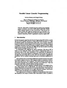
should be run. After iterating the program once, the new image is copied back and used as the source image, so that it can be operated on by subsequent iterations. An instruction in the function set allows the evolved program to know what iteration it is currently on, and potentially use this information to direct program flow. III. E XPERIMENT OVERVIEW The original input images (Figure 1) were combined together to form a larger image. A filter was applied using GIMP. We then used the evolutionary algorithm to find the mapping between the input image and the output images. The fitness function attempts to minimize the error between the desired output (the GIMP processed image) and the output from the evolved filters. The genetic programming technique is described fully in the following section. Section V describes the implementation of this algorithm and the fitness function on the GPU. The parameters and function set are given in Section VI. The choice of function set is determined by the functions available in the MS Accelerator API. Fig. 1. The training and validation image set. All images are presented simultaneously to the GPU. The first column of images is used to compute the validation fitness, the remaining twelve for the training fitness. Each image is 256 by 256 pixels, with the entire image containing 1024 by 1024 pixels.

Since FPGA based approaches are limited to binary operations, using a GPU we are able to work using floating point numbers - which makes direct comparison difficult. FPGA implementations also suffer from the need for specialist hardware and software skills. Evolved image filters have already been applied to a real world problem [7]. There programs were evolved to produce filters that could detect the changes between two images, for the detection of mud slides. The programs had to be insensitive to noise and other artifacts in the supplied images. Another use for genetic programming in image operations is for automatic feature extraction [12]. However, we consider these types of applications to be distinct from the one presented in this paper. A. Our Approach The approach we employ here is similar to the one in reference [2], where noise reduction filters were evolved. In this paper we expand that work, but into a more general purpose approach. In [2] we used 4 images for our training, and none for validation. Here we use 16 different images (Figure 1), that are largely taken from the USC-SIPI image repository. With 12 used for fitness evaluation, and 4 for validation. This allows us to be confident that evolved filters will generalise well. As we are employing the GPU for acceleration, we are able to test all the images at the same time (see section V) and obtain both the fitness score and the validation score at the same time. In this work, we allow the filters to be iterated. Evolution is allowed to determine how many times the evolved program

IV. C ARTESIAN G ENETIC P ROGRAMMING Cartesian Genetic Programming was originally developed by Miller and Thomson [5] for the purpose of evolving digital circuits and represents a program as a directed graph. One of the benefits of this type of representation is the implicit re-use of nodes in the directed graph. The technique is also similar to Parallel Distributed GP, which was independently developed by Poli [6], and also to Linear GP developed by Banzhaf[15]. Originally CGP used a program topology defined by a rectangular grid of nodes with a user defined number of rows and columns. However, later work on CGP always chose the number of rows to be one, thus giving a one-dimensional topology, as used in this paper. In CGP, the genotype is a fixed-length representation and consists of a list of integers which encode the function and connections of each node in the directed graph. CGP uses a genotype-phenotype mapping that does not require all of the nodes to be connected to each other, resulting in a bounded variable length phenotype. This allows areas of the genotype to be inactive and have no influence on the phenotype, leading to a neutral effect on genotype fitness called neutrality. This unique type of neutrality has been investigated in detail [5], [14], [16] and found to be extremely beneficial to the evolutionary process on the problems studied. Each node in the directed graph represents a particular function and is encoded by a number of genes. The first gene encodes the function the node is representing, and the remaining genes encode the location where the node takes its inputs from, plus one parameter that is used as a constant. Hence each node is specified by 4 genes. The genes that specify the connections do so in a relative form, where the gene specifies how many nodes back to connect[3]. If this address is negative, a node connects to an input. Modulo

arithmetic is used to handle conditions where the index goes beyond the number of inputs. The graph is executed by recursion, starting from the output nodes down through the functions, to the input nodes. In this way, nodes that are unconnected are not processed and do not effect the behavior of the graph at that stage. For efficiency, nodes are only evaluated once with the result cached, even if they are connected to multiple times. To clarify, figure 2 shows an example CGP program applied as a filter. The genotype for such a graph would be: ADD 2 6 4.35 MIN 1 7 2.3 MULT 3 8 3.2 ADD 1 2 -54 MAX 2 13 1.23 In addition, each individual in our population also stores an integer that specifies the number of times filter is applied. This iteration counter is bounded between 1 and 5. We chose to use CGP as in addition to having experience in using it, it provides some features such as bounded length programs and shared sub-trees that are useful on the constrained GPU platform. These can reduce the amount of memory (and processing) required to perform a given task. V. GPU I MPLEMENTATION A. General Requirements Graphics processors are specialized stream processors used to render graphics. Typically, the GPU is able to perform graphics manipulations much faster than a general purpose CPU, as the graphics processor is specifically designed to handle certain primitive operations. Internally, the GPU contains a number of small processors that are used to perform calculations on 3D vertex information and on textures. These processors operate in parallel with each other, and work on different parts of the problem. First the vertex processors calculate the 3D view, then the shader processors paint this model before it is displayed. Programming the GPU is typically done through a virtual machine interface such as OpenGL or DirectX which provide a common interface to the diverse GPUs available thus making development easy. However, DirectX and OpenGL are optimized for graphics processing, hence other Application Programming Interfaces (APIs) are required to emply the GPU as a general purpose device. Here we use the Microsoft Accelerator tool to provide a layer of abstraction between the evolutionary algorithm and the underlying API, drivers and hardware [11], [10]. B. Running Filters on a GPU Running the filters on the GPU will allow us to apply the kernel to every pixel (logically, but not physically) simultaneously. The parallel nature of the GPU will allow for multiple kernels to be calculated at the same time. This number will be dependent on the number of shader processors available. Using the Microsoft Accelerator architecture, it will appear to be completely parallel, although internally, the task will be broken down into chunks suitable for the GPU.

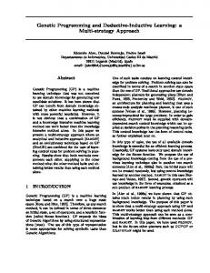
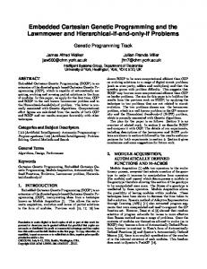
The image filter is made of an evolved program that takes a pixel and its neighbourhood (a total of 9 pixels) and computes the new value of that centre pixel. On a traditional processor, one would iterate over each pixel in turn and execute the evolved program each time. Using the parallelism of the GPU, many pixels (in effect all of them) can be operated on simultaneously. Hence, the evolved program is only evaluated once. Although the evolved program actually evaluates the entire image at once, we can break down the problem and consider what is required for each pixel. For each pixel, we need a program that takes it and it’s neighbourhood, and calculates a new pixel value. Therefore, the evolved program requires as many inputs as there are pixels in the neighbourhood and a single output. In the evolved program, each function has two inputs and one output. These inputs are floating point numbers that correspond to the grey level values of the pixels. Figure 2 illustrates a program that takes a 9 pixel sub image, and computes a new pixel value. Mapping the image filtering problem to the parallel architecture of the GPU is relatively straightforward. It is important to appreciate that the GPU typically takes 2 arrays and produces a 3rd by performing a parallel operation on them. The operation is element-wise, in the same way as matrix operations. To clarify, consider 2 arrays: a = [1, 2, 3] b = [4, 5, 6]. If we perform addition, we get c = [5, 6, 9]. With the SIMD architecture of the GPU, it is difficult to do an operation such as add the first element of one array to the second of another. To do such an operation, the second array would need to be shifted to move the element in the second position to the first. For the image filtering, we need to take a sub image from the main image as inputs for a program (our convolution kernel) - keeping in mind the matrix like operations of the GPU. To do this we take an image (e.g. the top left array in Figure 3) and shift the array one pixel in all 8 possible directions. This produces a total of 9 arrays (labeled (a) to (i) in Figure 3). Taking the same indexed element from each array will return the neighbourhood of a pixel. In the figure, the neighbourhood is shaded grey and a dotted line indicates how these elements are aligned. The GPU runs many copies of the evolved program in parallel, and essentially each program can only act on one array index. By shifting the arrays in this way, we have lined up the data so that although each program can only see a given array position, by looking at the set of arrays (or more specifically a single index in each of the arrays in the set) it can have access to the a given pixel and its neighbourhood becoming the inputs to our evolved program. For example, if we add array e to array i the new value of the centre pixel will be 6 - as the centre pixel in e has value 5 and the centre pixel in i has value 1. It is important to note that the evolutionary algorithm itself remains on the CPU, and only the fitness function is run on the GPU.

Fig. 2. In this example, the evolved program has 9 inputs - that correspond to a section of an image. The output of the program determines the new colour of the centre pixel. Note that one node has no connections to it’s output. This means the node is redundant, and will not be used during the computation.

Fig. 3. Converting the input image to a set of shifted images allows the element-wise operations of the GPU access a pixel and its neighbourhood. The evolved program treats each of these images as inputs. For example, should the evolved program want to sum the centre pixel and its top-left neighbour, it would add (e) to (i).

C. Fitness Function For the fitness function, we compute the average of the absolute difference between the target image and the image produced using CGP. The lower this error, the closer our evolved solution is to the desired output. Using the GPU, we can obtain both the training and validation fitness at the same time. This reduces some of the overhead of moving images and evolved programs to the GPU, and returning the fitness. We take the output from the evolved program, subtract it from our desired output and then its absolute value is calculated. This provides an array containing the difference of the two images. Next a mask is applied to remove the edges where the sub-images meet. This is done because when the images are shifted, we will be overlapping data from different images, and could introduce undesirable artifacts to the fitness computation. Edges are removed by multiplying the difference array by an array containing 0s and 1s. The 1s label where we wish to measure the difference. To calculate the training error, we multiply the difference

array by another mask. This mask contains 1s for each pixel in the training images, and 0 for pixels we do not wish to consider. We then sum the content of the array, and divide by the number of pixels to get the fitness value. A similar mask can then be used to find the validation fitness. VI. G ENETIC A LGORITHM AND PARAMETERS The algorithm used here is a simple evolutionary algorithm. We have a population of size 25. The mutation rate is set to be 5%, i.e. each gene in the genotype will be mutated with probablity 0.05. We do not use crossover. The iteration counter is also mutated with a 5% probability. The counter is mutated by adding a random number in the range -2 to 2. The counter is bounded between 1 and 5. Selection is done using a tournament selection of size 3. The 5 best individuals are promoted to the next generation without modification. The CGP graph is intialised to contain 100 nodes (it is important to note that not all nodes will be

Function ITERATION ADD SUB MULT DIV ADD CONST MULT CONST SUB CONST DIV CONST SQRT POW COS SIN NOP CONST ABS MIN MAX CEILING FLOOR FRAC LOG2 RECIPRICAL RSQRT

Description Returns the current iteration index Add the two inputs Subtract the second input from the first Multiply the two inputs Divide the first input by the second Adds a constant (the node’s parameter) to the first input Multiplies the first input by a constant (the node’s parameter) Subtracts a constant (the node’s parameter) to the first input Divides the first input by a constant (the node’s parameter) Returns the square root of the first input Raises the first input to the power of the second input Returns the cosine of the first input Returns the sin of the first input No operation - returns the first input Returns a constant (the node’s parameter) Returns the absolute value of the first input Returns the smaller of the two inputs Returns the larger of the two inputs Rounds up the first input Rounds down the first input Returns the fractional part of number, x - floor(x) Log (base 2) of the first input Returns 1/f √irstinput Returns 1/ f irstinput TABLE I CGP F UNCTION SET

used in the generated program). Evolution was allowed to run for 50,000 evaluations. Table I shows the available functions. The functions operate upon floating point numbers. VII. R ESULTS The results for evolving each filter are summarised in Table II. In the following sections, the best validation result is shown, alongside the output of the target filter from GIMP. We include examples of the evolved programs to illustrate the type of operations that evolution found to replicate the target filters. Due to space constraints, we are unable to include such analysis for every filter type. For implementation of the original filters, there is extensive coverage in the literature and also in the source code for GIMP. A. Dilatation and Erosion Figure 4 shows the result of evolving the ’Dilate’ filter. In ’Dilate2’ (figure 5), the filter is applied twice. Figure 6 shows the result of evolving the ’Erode’ filter. In ’Erode2’ (figure 7), the filter is applied twice. We can analyse the evolved program to determine how the filter works. For erosion, the best evolved program contains 8 operations and requires 5 iterations to run. The evolved expression is: Output = Max ( Log2 (I8 ) , Min ( I8 + (Min(I3 ,I7 )-Max(I7 ,I8 )), Floor(I1 )) ) Where I1 to I9 are the input pixels, as shown in figure 3. The best dilation program contains 4 instructions, and again requires 5 iterations. The evolved program is : Output = Max(Max(I9, Max(I1 ,I5 )),Max(I3 ,I7 ))

In contrast, the best evolved program for applying both erosion and dilation twice, both contain 17 instructions (and again require 5 iterations). It is unclear why these programs should need to be so much more complicated. B. Emboss, Sobel and Neon The Emboss, Sobel and Neon filters are different types of edge detectors. We chose to evolve these different types as the outputs are very different. Emboss is a directional filter, where as Sobel and Neon are not. We found that all three types of filters could be accurately evolved. Figure 8 shows the result of evolving the emboss filter. We find when that visually compared the evolved emboss filter is very similar to that used by GIMP (for this and the other sample images here, the most representative and visually useful sub image is used). The evolved program to evolve this filter contains 20 nodes: Output = ABS( MIN(-0.3857, POW(SQRT(I2 /((I8 +RSQRT(I5 ))-0.863)),I8)) + CEIL(MIN(((I3-I9 )+(I1 -I7 )) -129.65,FRAC(I5)))) Figure 9 shows the result of evolving the neon filter. GIMP has two versions of the Sobel filter. Figure 10 shows the result of evolving a normalized ’Sobel’ filter. In ’Sobel2’ (Figure 11), the target was the standard Sobel filter. The standard Sobel filter receives poor error rates, however the visual comparison is very good. It would appear that the evolved output is scaled differently, and hence the pixel intensities are different. If both images are normalized, the error is reduced. However, our fitness function does not normalize automatically, and leaves this task to evolution. The evolved Sobel filter is quite complicated:

Filter Dilate Dilate2 Emboss Erode Erode2 Motion Neon Sobel Sobel2 Unsharp

Best error 0.57 5.84 3.86 0.56 5.70 2.08 1.32 8.41 1.70 5.85

Avg Validation Error 0.71 6.51 8.33 0.78 6.72 2.32 2.69 22.26 3.82 5.91

Avg Validation Evals 2422 11361 15517 3892 26747 29464 15836 26385 19979 301

Avg Train Error 0.67 6.10 7.41 0.73 6.64 2.24 2.41 20.12 3.55 5.61

Avg Train Evals 3919 39603 34878 4066 40559 43722 35146 45744 39155 37102

TABLE II R ESULTS PER EVOLVED FILTER . ‘B EST ERROR ’ IS THE LOWEST ERROR SEEN WHEN TESTING AGAINST THE VALIDATION IMAGES . ’ AVG VALIDATION E RROR ’ IS THE AVERAGE OF THE BEST VALIDATION ERROR . ’AVG VALIDATION E VALS ’ IS THE AVERAGE NUMBER OF EVALUATIONS REQUIRED TO FIND THE BEST VALIDATION ERROR . ’AVG T RAIN E RROR ’ IS THE AVERAGE OF THE LOWEST ERROR FOUND ON THE TRAINING IMAGES . ’AVG T RAIN E VALS ’ IS THE AVERAGE NUMBER OF EVALUATIONS REQUIRED TO FIND THE BEST TRAINING FITNESS . E ACH EXPERIMENT WAS REPEATED FOR 20 TRIALS .

A = I7 - I3 B = I9 - MAX(I1 ,LOG2 (A)) OUTPUT = 2.0 * (MIN(MAX(ABS(B)+FRAC(1)+ABS(2.0 * A), MAX(FLOOR(LOG2 (A)),2.0 * B)), (CEIL(FRAC(I5 )) * -0.760)+127.24)) The best evolved program for Sobel2 was considerably shorter: Output = Max (ABS((I9 - I1 ) * 0.590), POW(I3 - I7,SQRT(0.774)) / -2.245) Again, both programs required 5 iterations. This suggests there is some bias in the algorithm to increase the number of iterations to the maximum allowed. C. Motion blur Figure 12 shows the result of evolving the motion filter. The output of the evolved filter did not match the desired target very accurately. Although there is a degree of blurring, it is not as pronounced as in the target image. Motion blur is a relatively subtle effect, and as the target and input images are quite similar, it is likely that evolution will become trapped in a local minima. D. Unsharp Figure 13 shows the result of evolving the ’Unsharpen’ filter. Unsharpen was the most difficult filter to evolve. We suspect this is due to the Gaussian blur that needs to be applied as part of the procedure. It is difficult to see how, with the current function set, such an operation can evolve. We will need to rectify this in future work. VIII. GPU P ERFORMANCE Using the Graphics Processor greatly decreases the evaluation time per individual. On our test system (NVidia 8800 GTX, AMD Athlon 3500+, Microsoft Accelerator API), we obtained approximately 145 million Genetic Programming Operations Per Second (GPOps), and a peak performance of 324 Million GPOps. The processing rate is dependent on the length of the evolved programs. Some filters benefit more from the GPU implementation than others.

At present, it is unclear of the relationship of this figure to Floating Point Operations Per Second. Executing the evolved programs using the CPU bound reference driver, we obtain only 1.2 million GPOps, i.e. a factor of 100 times slower than the GPU. However, using the reference driver incurs significant overhead and may not be an accurate reflection of the true speed of the CPU. The high processing rate suggests that this technique may also be suitable for real time image processing, and the possibility of continual adaptation. We hope to explore this problem in a future paper. We also investigated the performance of applying a small number of images, i.e. 4 instead of 16. We found that the processing time was the same, suggesting that there is a large overhead of moving images to the GPU. IX. C ONCLUSIONS In this paper we have demonstrated that it is possible to use genetic programming to reverse engineer image processing algorithms. We have also demonstrated that such techniques are well suited for implementation on GPUs. Using the GPU greatly speeds up evaluation, and allows for a more robust fitness test - as multiple images, with different properties, can be used. The increased evolutionary power also allowed us the opportunity to investigate the evolution of some more unconventional filters that have yet to be used as problems in the genetic programming community. We expect that our technique could be used to reverse engineer proprietary image processing algorithms. Assuming that a user has access to the unprocessed version of the image, it should be possible to discover an algorithm that replicates the original processing technique. Such a system could be practical in providing open source versions of closed source products. Another possible use is to optimise existing hand design processes. By first designing a procedure by hand, the system could then be used to find an equivalent filter. It should be possible to evolve filters that require fewer operations, as the GP would automatically be able to reduce multiple conventional convolutions into a single program.

Filter Dilate Dilate2 Emboss Erode Erode2 Motion Neon Sobel Sobel2 Unsharp

Peak GPOps 116 281 254 230 307 280 266 292 280 324

Avg GPOps 62 133 129 79 195 177 185 194 166 139

TABLE III M AXIMUM AND AVERAGE G ENETIC P ROGRAMMING O PERATIONS P ER S ECOND (GPO PS ) OBSERVED FOR EACH FILTER TYPE .

R EFERENCES [1] GNU. Gnu image manipulation program (GIMP). www.gimp.org, 2008. [Online; accessed 21-January-2008]. [2] S. Harding. Evolution of image filters on graphics processor units using cartesian genetic programming. In IEEE World Congress on Computational Intelligence, WCCI 2008, Hong Kong, China, June 16, 2008, volume 5050 of Lecture Notes in Computer Science, pages 1921–1928. Springer, 2008. [3] S. Harding, J. F. Miller, and W. Banzhaf. Self-modifying cartesian genetic programming. In H. Lipson, editor, GECCO, pages 1021–1028. ACM, 2007. [4] P. N. Kumar, S. Suresh, and J. R. P. Perinbam. Digital image filter design using evolvable hardware. In ICIS ’05: Proceedings of the Fourth Annual ACIS International Conference on Computer and Information Science (ICIS’05), pages 483–488, Washington, DC, USA, 2005. IEEE Computer Society. [5] J. F. Miller and P. Thomson. Cartesian genetic programming. In R. Poli and W. B. et al., editors, Proc. of EuroGP 2000, volume 1802 of LNCS, pages 121–132. Springer-Verlag, 2000. [6] R. Poli. Parallel distributed genetic programming. In D. Corne, M. Dorigo, and F. Glover, editors, New Ideas in Optimization. McGrawHill, 1999. [7] P. Rosin and J. Hervas. Image thresholding for landslide detection by genetic programming. Analysis of multi-temporal remote sensing images, pages 65–72, 2002. [8] K. Slan and L. Sekanina. Fitness landscape analysis and image filter evolution using functional-level cgp. Lecture Notes in Computer Science, 2007(4445):311–320, 2007. [9] S. L. Smith, S. Leggett, and A. M. Tyrrell. An implicit context representation for evolving image processing filters. In F. Rothlauf, J. Branke, S. Cagnoni, D. W. Corne, R. Drechsler, Y. Jin, P. Machado, E. Marchiori, J. Romero, G. D. Smith, and G. Squillero, editors, Applications of Evolutionary Computing, EvoWorkshops2005: EvoBIO, EvoCOMNET, EvoHOT, EvoIASP, EvoMUSART, EvoSTOC, volume 3449 of LNCS, pages 407–416, Lausanne, Switzerland, 30 Mar.-1 Apr. 2005. Springer Verlag. [10] D. Tarditi, S. Puri, and J. Oglesby. Accelerator: using data parallelism to program GPUs for general-purpose uses. In ASPLOS-XII: Proceedings of the 12th international conference on Architectural support for programming languages and operating systems, pages 325–335, New York, NY, USA, 2006. ACM. [11] D. Tarditi, S. Puri, and J. Oglesby. Msr-tr-2005-184 accelerator: Using data parallelism to program GPUs for general-purpose uses. Technical report, Microsoft Research, 2006. [12] L. Trujillo and G. Olague. Synthesis of interest point detectors through genetic programming. In GECCO ’06: Proceedings of the 8th annual conference on Genetic and evolutionary computation, pages 887–894, New York, NY, USA, 2006. ACM. [13] Z. Vacek and L. Sekanina. Evaluation of a new platform for image filter evolution. In Proc. of the 2007 NASA/ESA Conference on Adaptive Hardware and Systems, pages 577–584. IEEE Computer Society, 2007. [14] V. K. Vassilev and J. F. Miller. The advantages of landscape neutrality in digital circuit evolution. In Proc. of ICES, volume 1801, pages 252–263. Springer-Verlag, 2000. [15] G. Wilson and W. Banzhaf. A comparison of cartesian genetic programming and linear genetic programming. In Proceedings of the 11th

European Conference on Genetic Programming (EuroGP 2008), volume 4971, pages 182–193. Springer Berlin, 2008. [16] T. Yu and J. Miller. Neutrality and the evolvability of boolean function landscape. In J. F. Miller and M. T. et al., editors, Proc. of EuroGP 2001, volume 2038 of LNCS, pages 204–217. Springer-Verlag, 2001.

Fig. 4.

Fig. 5.

Dilate: Evolved filter and GIMP filter

Dilate twice: Evolved filter and GIMP filter

Fig. 6.

Erode: Evolved filter and GIMP filter

Fig. 10.

Sobel: Evolved filter and GIMP filter

Fig. 7.

Erode2: Evolved filter and GIMP filter

Fig. 11.

Sobel2: Evolved filter and GIMP filter

Fig. 8.

Emboss: Evolved filter and GIMP filter

Fig. 12.

Motion blur: Evolved filter and GIMP filter

Neon blur: Evolved filter and GIMP filter

Fig. 13.

Unsharp blur: Evolved filter and GIMP filter

Fig. 9.