ABSTRACT. We study the distributed Kalman filter in sensor networks where multiple sensors collaborate to achieve a common objective. Our motivation is to ...
DISTRIBUTED KALMAN FILTERS IN SENSOR NETWORKS: BIPARTITE FUSION GRAPHS Usman A. Khan and Jos´e M. F. Moura Carnegie Mellon University Department of Electrical and Computer Engineering Pittsburgh, PA 15213 {ukhan, moura}@ece.cmu.edu ABSTRACT We study the distributed Kalman filter in sensor networks where multiple sensors collaborate to achieve a common objective. Our motivation is to distribute the global model that comes from the statespace representation of a sparse and localized large-scale system into reduced coupled sensor-based models. We implement local Kalman filters on these reduced models, by approximating the Gaussian error process of the Kalman filter to be Gauss-Markov, ensuring that each sensor is involved only in reduced-order computations and local communication. We propose a generalized distributed Jacobi algorithm to compute global matrix inversion, locally, in an iterative fashion. We employ bipartite fusion graphs in order to fuse the shared observations and shared estimates across the local models. Index Terms— Large-scale systems, Sparse matrices, Distributed algorithms, Matrix inversion, Kalman filtering 1. INTRODUCTION Recent technological advances in solid-state electronics and wireless communication have made it possible to monitor very largescale dynamical systems, e.g., power grid, weather forecast systems, and earthquake tracking systems, using sensor networks. These geographically distributed sensors take measurements of the variables pertinent to the system. These measurements, in addition to be employed in other tasks, are used for state estimation. State estimation is essential to these dynamical systems for control, tracking and navigational purposes. We develop a distributed Kalman filter for the multisensor large-scale dynamical systems with localized and sparse structure. With sensor networks the observations of the field of interest are distributed across different sensors. All these observations are to be incorporated in the implementation of the Kalman filter to ensure optimal performance. Collecting these observations at a single location (fusion center) implements a centralized Kalman filter. The fusion center then communicates the estimates back to the sensors. In large-scale dynamical systems, the centralized Kalman filter is impractical because it requires: (i) long-distance communication since the sensors span a large geographical area; and (ii) high computation because the state-space models coming from such large-scale systems have high-dimensional state vectors. Furthermore, a centralized scheme has the disadvantages of large latency and a single point of failure. This work was partially supported by the DARPA DSO Advanced Computing and Mathematics Program Integrated Sensing and Processing (ISP) Initiative under ARO grant # DAAD 19-02-1-0180, by NSF under grants # ECS-0225449 and # CNS-0428404, and by an IBM Faculty Award.
1-4244-1198-X/07/$25.00 ©2007 IEEE
700
To reduce the inordinate communication requirements, Kalman filters have been implemented by replicating the global model at each sensor. This is still computationally expensive involving nth order matrices and vectors (where n is the dimension of the large-scale system). Much of the existing research addresses this problem of reducing the communication burden, but, by replicating the nth order global dynamics at each sensor, which, in general, requires O(n3 ) computations. In this paper, we present a solution that reduces the communication as well as the computation requirements. In our approach, we distribute the global dynamics into reduced-order local dynamics. This reduces the computational burden at each sensor, since the computations are of the order of the local reduced-order models, nl , where nl � n. We devise local Kalman filters that are efficient for large-scale systems and avoid at each sensor the drawbacks, extensive computation and inordinate communication, of the centralized implementation. Decentralizing Kalman filter dates back to [2, 3, 4], requiring all-to-all communication networks and nth order replicated models. A decentralized Kalman filter where the observations are fused using local communication and iterative consensus filters is provided in [5]. Distributing the communication requirements in the presence of uncertain communication links and packet losses is addressed in [6], where the problem of target tracking is considered, see also [7]. The problem of target tracking requires a few state variables, e.g., velocity and acceleration, and has an inherent structure of decoupled dynamics in the case of multiple targets. All these decentralized schemes reduce the communication burden but replicate the nth order Kalman filter at each sensor with O(n3 ) computational requirements, a practically infeasibility when n is large. Kalman filters with reduced models were addressed in [8]. This work was further extended in [9]. In their work, the reduced models at each sensor are decoupled, forcing the model matrix to be block diagonal. Furthermore, the network topology is either fully connected, [8], or is close to fully connected, [9], requiring long distance links that are expensive. Willsky et. al. [10], have also addressed the problem of combining estimates from the subsystems of a global system, but in their implementation the local sub-systems are decoupled, making the sub-systems independent Markov processes. This solution does not address the problem we consider here of coupled large-scale dynamical systems. We present a fully distributed Kalman filter, implemented on sensor-based reduced models and distributed observations. In order to achieve this, we distribute the state-space models coming from the large-scale dynamical systems, into reduced coupled sensor-based models at each sensor1 . These reduced models exploit the localized 1 We assume that the state-space model cannot be decoupled under any model preserving transformation of the state vector.
SSP 2007
and sparse structure of the system dynamics2 . Local Kalman filters are then implemented on the reduced models. Each local Kalman filter computes local variables, a subset of the global variables (state, observations, error covariances) required in its centralized counterpart. Hence the computations required at the sensors are significantly reduced. Coupling between the reduced models is preserved and global performance is achieved by exchanging messages across different sensors using only local communication. We distribute the Information filter form of the Kalman filter3 . In the process, we assume information matrices in the Information filter to be L-banded (we refer to a matrix as an L-banded matrix (L ≥ 0), if the elements outside the band defined by the Lth upper and Lth lower diagonal are zero.) This assumption is equivalent to forcing the Gaussian error processes to be Gauss-Markovian and is optimal in Kullback-Leibler or maximum entropy sense [12]. This assumption helps us in making the computations and communications to be local. It will be shown that without this assumption a distributed implementation is not possible, requiring either global communication or computing global variables. Simulations in [13] show that the centralized Information filter with L-banded approximations is virtually indistinguishable from the exact centralized Information filter. We provide the global model and centralized Information filter in sections 2 and 3, respectively. We will discuss the sensor-based reduced models in section 4. The local Information filters are divided in section 5 and section 6, with results and conclusions in section 7.
where we have
2 6 yk = 6 4
(1)
yk .. . (N ) yk
3 7 7 5,
2 6 H=4
H1 .. . HN
2 6 wk = 4
3 7 5,
(4)
H E[uk uH j ] = Qδij and E[wk wj ] = Rδij .
3. CENTRALIZED INFORMATION FILTER The estimator and the predictor in the Information filter domain are
bzk|k = Zk|k xbk|k , and bzk|k−1 = Zk|k−1 xbk|k−1 , respectively, where
the Information matrices, Zk|k , and Zk|k−1 , are the inverses of the estimation error covariance matrix, Sk|k , and prediction error covariance matrix, Πk|k−1 , respectively. Let the nth-dimensional global observation variables be ik = HT R−1 yk and Ik = HT R−1 H and (l) the nth-dimensional local observation variables be il,k = HTl R−1 l yk −1 T and Il,k = Hl Rl Hl . It can be shown that [9]
2. GLOBAL MODEL
Ik
(1)
where k is the discrete time index, xk ∈ Rn is the state vector, F ∈ Rn×n is a sparse localized model matrix, uk ∈ Rm is the state noise vector and G ∈ Rn×m is the state noise matrix, and x0 are the initial conditions such that x0 ∼ N (x0 , Σ0 ). We assume that the random field (1), is monitored by N sensors. Observations at sensor l are, (l)
(l)
yk = Hl xk + wk ,
(5)
We also note that R = blockdiag[R1 , . . . , RN ].
=
N X
(l)
HTl R−1 l yk =
l=1
xk+1 = Fxk + Guk ,
3 75 .
We adopt the standard assumptions on the statistical characteristics of the white noise sequences, {uk }k≥0 , and {wk }k≥0 , with
ik
We assume that the dynamical system follows an n-dimensional state equation
(1)
wk .. . (N ) w
=
N X
N X
il,k
(6)
Il,k
(7)
l=1
HTl R−1 l Hl =
N X
l=1
l=1
The centralized Information filter equations for the global model (1) and (3) contain initial conditions, a filter step, and a prediction step. z0|−1 = Z0|−1 x0 . The The initial conditions are Z0|−1 = Σ−1 0 and b filter step of the centralized Information filter is given by Zk|k
=
N X
Zk|k−1 +
Il,k ,
(8a)
il,k .
(8b)
l=1
bzk|k
(2)
bzk|k−1 +
=
N X l=1
where Hl ∈ Rpl ×n is the local observation matrix, and w(l) ∈ Rpl is the local observation noise with the covariance matrix, Rl . We can get the global observation model by stacking the observations at each sensor in a global observation vector, yk ∈ Rp×n given by
The prediction step of the centralized Information filter is given by
yk = Hxk + wk ,
4. SENSOR-BASED REDUCED MODELS
(3)
2 Sparse dynamical systems span a large variety of interesting applications, e.g., image reconstruction problem where the pixel values depend on the neighboring pixels, random fields obtained by discretizing PDEs, power grids. Localized structure on the global dynamics refers to systems where the correlations among the states farther apart in the state vector decay rapidly. A broad range of sparse systems, not exhibiting the localized structure, can be converted into sparse banded systems with highly localized structures, using parallelized iterative solvers, e.g., Reverse Cuthill Mckee (RCM) reordering, [11]. 3 Information filters [9], are algebraically equivalent to the Kalman filter [1]. In Information filters the information matrices (inverse of the error covariance matrices) are iterated at each time step.
701
Zk|k−1
=
−1 T T −1 Π−1 , (9a) k|k−1 = (FZk−1|k−1 F +GQG )
bzk|k−1
=
zk−1|k−1 . Zk|k−1 FZ−1 k−1|k−1 b
�
�
(9b)
In this section, we present the model distribution in order to obtain reduced sensor-based models at each sensor. At the lth sensor, we choose an nl × n selection matrix, Tl , see also [9], such that it (l) chooses the nl local states in the local state vector, xk , from the global state vector, xk , (l)
xk = Tl xk .
(10)
The choice of the selection matrix, Tl , is such that, if a sensor l observes a linear combination of states through the local observation (l) matrix, Hl , all these states are included in the local state vector, xk .
For example, if we have a 5-dimensional system with sensor l having the local observation matrix,
� Hl =
h11 0
h12 h22
0 h23
0 0
0 0
x1
x2
x3
x4
s1
s2
s3
x5
� ,
(11)
the selection matrix is,
2
1 Tl = 4 0 0
0 1 0
0 0 1
3
0 0 0
0 0 5. 0
(12)
A detailed model distribution procedure for obtaining reduced order sensor-based models using a graph theoretic approach is provided in (l) [14]. The reduced model at sensor l involves xk as a local state vector. Putting (10) in (1) and defining Fl = Tl F and Gl = Tl G, we have (l)
xk+1 = Fl xk + Gl uk
(13)
We partition Fl into a reduced model matrix, F(l) , which corre(l) sponds to the reduced state vector, xk , and an input matrix, D(l) , which corresponds to the rest of the states not included in the re(l) duced state vector, xk (these states that are not included will be the inputs to the reduced model so that we can preserve the coupling and in turn the global model). Notice that, since the model matrix, F, is sparse and localized, most of the columns in D(l) will be zero and we retain only its non zero columns, with their corresponding states (l) in an input vector, dk . We also retain only the state noise sources relevant to the reduced model. Now the reduced model at sensor l becomes (l)
xk+1 (l) yk
= =
(l)
(l)
(l)
F(l) xk + D(l) dk + G(l) uk H
(l)
(l) xk
+
(l) wk
Fig. 1. Bipartite fusion graph for a 5-dimensional system with the global and local observation matrices of equation (17).
(14) (15)
Note that the reduced local observation matrix, H(l) ∈ Rpl ×nl is different from the local observation matrix, Hl ∈ Rpl ×n . The term (l) D(l) dk in (14), arises because the local model at sensor l is coupled to the local models at those neighboring sensor (recall F is sparse (l) and localized), which model the states, in dk , in their local model. If we ignore this term, we reduce our model to decoupled local subsystems as in [10, 9]. We do not ignore this coupling and require it (l) to be communicated from the neighboring sensors. Because dk is (l) b as inputs, which is communicated from not available, we use d k|k the neighboring sensors that are modeling the states in the vector dk , in their reduced models. The local Information filters are now based on (14) and (15). The local Information filters contain a local filter step and local prediction step, divided in the next sections. The local filter step (section 5) requires observation fusion and estimate fusion because reduced models across different sensors may have overlapping states. The fusion is carried out with the help of bipartite fusion graphs, section 5.1. The local prediction step (section 6) requires a global variable because the reduced models are coupled; we avoid computing this global variable by using iterative generalized distributed Jacobi algorithms. 5. LOCAL FILTER STEP (l)
Define nl th-dimensional reduced local observation variables ik = (l) (l) −1 (l) (l) T (H(l) )T R−1 l yk and Ik = (H ) Rl H . Then the local filter
702
step is given by (l)
Zk|k (l) zk|k
b
(l)
(l)
=
Zk|k−1 +If,k ,
(16a)
=
(l) (l) zk|k−1 +if,k ,
(16b)
b
(l)
(l)
where the fused observation variables If,k and If,k are discussed in section 5.1.1.We go from the estimates in the Information filter do(l) b(l) main, b zk|k to the estimates in the Kalman filter domain, x k|k , by bk|k = b zk|k , which resolving a linear system of equations Zk|k x quires long distance communication and extensive computations for arbitrary estimation information matrices, Zk|k . If we approximate Zk|k to be an L-banded matrix ∀k, a solution with only local communication and computations with local variables is possible, using an iterative distributed Jacobi algorithm for vectors (DJV), see also [15]. 5.1. Bipartite Fusion Graphs After the model distribution step introduced in section 4, several sensors may share states in their reduced models (14). This is equiva(l) lent to saying that the local state vectors, xk , for all the sensors may overlap and hence the sensor-based reduced models share the overlapped states. Recall that the choice of the selection matrix, Tl , is based on the local observation matrices, Hl . So the sensors having shared states have different observations of the shared states. The observations corresponding to the shared states need to be fused in order to guarantee global performance. Since each sensor implements a separate local Information filter, the estimates corresponding to the shared states also need to be fused across the sensors containing those states. We implement the fusion procedure with the help of bipartite fusion graphs, introduced below. We present a simple example illustrating the bipartite fusion graphs. We can easily extend this illustration for the case of higher order state-vectors and a large number of sensors. Consider a 5dimensional system observed by N = 3 sensors, where the global observation matrix, H, composed by local observation matrices Hl , see equation (4), is given by
2
3
2
h11 H1 H = 4 H2 5 = 4 0 H3 0
h12 h22 0
0 h23 h23
0 h24 h24
3
0 0 5. h25
(17)
A bipartite fusion graph, B = [X ∪ S, E], where X = {xi }i=1,...,n is the state-set and S = {sj }j=1,...,N is the sensor-set, consists of
the partitioned vertex set, X ∪ S, and an interconnection matrix, E. The structure of the interconnection matrix, E, is imposed by the global observation matrix, H, in the following way. The sensor, si , is connected to the state variable, xj , if si observes the state variable, xj . In other words, we have an edge between the sensor, si , and the state variable, xj , if the local observation matrix, Hi , at sensor si , contains a non-zero in its jth column. The bipartite fusion graph, B, for the global observation matrix, H in (17), is shown in figure 1. The bipartite fusion graphs provides a natural way of selecting the sensors required in the fusion corresponding to each state. For example, figure 1 suggests that: for state x1 , no observation fusion or estimate fusion is required since it is observed and hence modeled only at sensor s1 ; for state x2 , observation fusion and estimate fusion is required on the sensors s1 and s2 ; and so on. In this way, we distribute the global observation into local observation fusion for each state, where only the information from neighboring sensors is required. We provide some notation for the next subsections. Let G be the sensor communication graph; this entails the sensor communication pattern. For each state, xj , let Gj be the induced subgraph of G, such that the vertices of Gj are all the sensors connected to the state, xj , in the bipartite fusion graph, B. It is obvious that, to properly carry out the fusion procedure, we require G and Gj ∀j to be connected. We present observation fusion in subsection 5.1.1 and estimate fusion in subsection 5.1.2.
5.1.2. Estimate Fusion (s)
For each state xj , each sensor s ∈ Gj has an estimate, x bj,k|k . If Gj contains more than one sensor, there are multiple correlated estimates of the same state, which should be fused in order to obtain an estimate with smaller variance, for vector extensions, see e.g., [10]. (s) At each sensor s ∈ Gj , let πj be the variance of the jth state esti(s)
(s)
error covariance matrix, Sk|k , at sensor s. We fuse the estimates using the parallel fusion of estimates formula, which can be derived by using Lagrange multipliers,
1−1 0 1 0 X � (s) �−1 X � (s) �−1 (s) A @ πj πj x bj,k|k A . (21) x bj,k|k = @ s∈Gj
6. LOCAL PREDICTION STEP We address the computation of the local prediction information ma(l) trix, Zk|k−1 , first. Following (9a), it can be shown that the local (l)
prediction error covariance matrix, Πk|k−1 , is given by (l)
With the help of the above discussion and (6), we establish the fusion of the local observation variables. Let the entries of the nl × 1 (l) reduced observation vector, ik , at sensor l, be subscripted by the nl state variables modeled at sensor l. In the context of our example system in (17) and figure 1, we have (1)
ik =
(1)
ik,x1 (1) ik,x2
#
2 (2) 3 2 (3) 3 ik,x2 i 3 7 , i(3) = 6 ik,x 7. 6 (2) , ik = 4 i(2) 4 (3) k k,x3 5 k,x4 5 (2)
(3)
ik,x4
ik,x5
(18)
For each state xj , the observation fusion is carried out on the sensors attached to this state in the bipartite fusion graph, B. The fused (2) observation vector, for instance at sensor 2 denoted by if,k , is given by 3 2 (2) (1) ik,x2 + ik,x2 7. 6 (2) (3) if,k = 4 i(2) (19) k,x3 + ik,x3 5 (2) (3) ik,x4 + ik,x4 (l)
Generalizing to the arbitrary sensor l, we may write the entry, if,k,xj , corresponding to xj in the fused observation vector, (l)
if,k,xj =
s∈Gj
Both sums in (21) can be carried out using the weighted averaging algorithm [16].
5.1.1. Observation Fusion
"
(s)
mate, x bj,k|k , where πj is a diagonal element in the local estimation
X
s∈Gj
(s)
ik,xj ,
(l) if,k ,
as (20)
(s)
where ik,xj is the entry corresponding to xj in the reduced observa(s)
tion vector at sensor s, ik . Since the communication network on Gj will not be, in general, all-to-all, an iterative weighted averaging algorithm [16] can be used to compute the fusion in (20) over arbitrarily connected communication networks with only local communication. A similar procedure on the pairs of state variables and their associated subgraphs, Gjm , (l) can be implemented to fuse the reduced observation matrices, Ik .
703
T (l) (l) (l)T . Πk|k−1 = Fl Z−1 k−1|k−1 Fl + G Q G
(22)
(l)
We need to go from a local matrix, Zk−1|k−1 , resulting from the local filter step (16), to a global matrix, Z−1 k−1|k−1 , in order to com(l)
pute Πk|k−1 from (22). This problem cannot be solved for arbitrary symmetric matrices, Zk−1|k−1 , since it will require long distance communication and an n × n matrix inverse, infeasible to implement at sensors. To achieve this, we use a generalized distributed Jacobi (GDJ) algorithm for banded matrix inversion presented elsewhere, which iterates on local matrices and requires local communication. A distributed Jacobi algorithm to solve a single linear system of equations with similar banded structure is presented in [15]. The GDJ we propose here solves matrix inversion (n coupled linear systems of equations), with only local computation and local communication using L-banded theorems from [13]. (l) (l) We need to go from Πk|k−1 (a submatrix in Πk|k−1 ) to Zk|k−1 (a submatrix in Zk|k−1 ), where Πk|k−1 = Z−1 k|k−1 . A solution with only local communication and computations with local matrices is possible, if we approximate the prediction information matrix, Zk|k−1 , to be an L-banded matrix ∀k, using the L-banded inversion theorem in [12]. The second part is to calculate the local transformed predicted (l) estimate, b zk|k−1 . Following (9b) and the transformations in section 3, it can be shown that (l) bk−1|k−1 , bzk|k−1 zk|k−1 = Tl Zk|k−1 Fx = Tl b
(23)
where the product Tl Zk|k−1 contains the nl rows of the prediction information matrix, Zk|k−1 , corresponding to the locally modeled states at sensor l. Here we recall that Zk|k−1 is an L-banded matrix, which helps us in computing (23) locally. Notice that if we do not use this assumption than the computation in (23) will require a linear bk−1|k−1 , which will recombination of arbitrary estimated states in x quire long distance communication. Depending on the value of L,
8. REFERENCES
10 8 6 4 2 0
−2 0
20
40 60 Information filter iterations
80
100
Fig. 2. Simulation Results: We show the original state variables (solid/blue) and their estimates using the the proposed scheme (dashdot/black), which are virtually indistinguishable from the optimal estimates using the centralized Information filter (dashed/red).
Tl Zk|k−1 will pick a linear combination of the entries in the vector bk−1|k−1 . Since the model matrix, F, has a localized/spare strucFx ture, the communication required will always be local. The communication might be multi-hop and will depend on the value of L. 7. RESULTS AND COCLUSIONS We simulate a 5 dimensional system monitored by 3 sensors. We implement the proposed scheme, with L = 1-banded approximation, and compare its performance with the centralized Information filter estimates, figure 2. The original state variables are shown as solid lines (blue). The optimal estimates, computed from the centralized Information filter, are shown as dashed lines (red). The estimates using the proposed scheme are shown as dash-dot lines (black), which are virtually indistinguishable from the centralized estimates (red/dashed). It can also be shown that the local L-banded Information filters and the centralized L-banded Information filters have the same performance. To conclude, we comment on the complexity of the distributed Kalman filter presented in the paper. The computational complexity of the centralized Information filter is O(n3 k) and for the Information filter with distributed observations in [5] is O((n3 + f (n)tc )k), where tc is the number of iterations required for the consensus algorithm [5] (with complexity, say O(f (n))) to converge. The computational complexity for the proposed scheme is O((n3l + n3l tJ1 + n2l tJ2 + n2l tw )k), where tJ1 , tJ2 and tw are the iterations required for DJV, GDJ, and weighted averaging algorithm to converge, respectively. Even for the toy-example simulated here, where n = 5 and n1 = 3, n2 = 3 and n3 = 2, the computational advantage at the sensors is evident. In this example, typical values for tJ1 , tJ2 and tw (we used local degree weights for observation fusion in [16] with a sensor communication network 1 ↔ 2 ↔ 3, other techniques e.g., semi-definite programming [16] can be used to decrease tw significantly) are 6, 7 and 9 respectively. The convergence rate of the iterative algorithms can be increased by optimizing the communication network topology [17].
704
[1] B. D. O. Anderson and J. B. Moore, Optimal Filtering, Prentice Hall, Englewoods Cliff, NJ, 1979. [2] J. L. Speyer, “Computation and Transmission requirements for a decentralized linear-quadratic-gaussian control problem,” IEEE Transactions on Automatic Control, vol. 24, no. 2, pp. 266–269, Feb 1979. [3] H. R. Hashemipour, S. Roy, and A. J. Laub, “Decentralized structures for parallel Kalman filtering,” IEEE Transactions on Automatic Control, vol. 33, no. 1, pp. 88–94, Jan. 1988. [4] B.S. Rao and H. Durrant-Whyte, “Fully decentralized algorithm for multisensor Kalman filtering,” in IEEE ProceedingsControl Theory and Applications, Sep. 1991, vol. 138, pp. 413– 420. [5] R. Olfati-Saber, “Distributed Kalman filters with embedded consensus filters,” in 44th IEEE Conference on Decision and Control, Dec. 2005, pp. 8179 – 8184. [6] M. Alanyali and V. Saligrama, “Distributed Tracking in Multi- Hop Networks with Communication Delays and Packet Losses,” in IEEE Workshop on Statistical Signal Processing, 2005, pp. 1190–1195. [7] T. H. Chung, V. Gupta, J. W. Burdick, and R. M. Murray, “On a Decentralized Active Sensing Strategy using Mobile Sensor Platforms in a Network,” in Proc. of the IEEE Conf. on Decision and Control, Paradise Island, Bahamas, Dec 2004. [8] T. Berg and H. Durrant-Whyte, “Model distribution in decentralized multi-sensor data fusion,” Tech. Rep., University of Oxford, 1990. [9] A. G. O. Mutambara, Decentralized Estimation and Control for multisensor systems, CRC Press, Boca Raton, FL, 1998. [10] A. Willsky, M. G. Bello, D. A. Castanon, B. C. Levy, and G. C. Verghese, “Combining and Updating of Local Estimates and Regional Maps Along Sets of One Dimensional Tracks,” IEEE Transactions on Automatic Control, vol. 24, no. 4, pp. 799– 813, 1982. [11] A. George and J. Liu, Computer Solution of Large Sparse Positive Definite Systems, Prentice Hall, 1981. [12] A. Kavcic and J. Moura, “Matrices with Banded Inverses: Inversion Algorithms and Factorization of Gauss-Markov Processes,” IEEE Transactions on Information Theory, vol. 46, no. 4, pp. 1495–1509, Jul. 2000. [13] A. Asif and J. Moura, “Inversion of Block matrices with LBlock Banded Inverse,” IEEE Transactions on Signal Processing, vol. 53, no. 2, pp. 630–642, Feb. 2005. [14] Usman A. Khan and Jos´e M. F. Moura, “Model Distribution for Distributed Kalman Filters: A Graph Theoretic Approach,” Submitted, 5 pages, Jun. 2007. [15] V. Delouille, R. Neelamani, and R. Baraniuk, “Robust Distributed Estimation using the Embedded Subgraphs Algorithm,” IEEE Transactions on Signal Processing, vol. 54, no. 8, pp. 2998–3010, Aug 2006. [16] L. Xiao and S. Boyd, “Fast linear iterations for distributed averaging,” in Systems and Controls Letters, 2004, pp. 65–78. [17] S. Aldosari and J. Moura, “Distributed Detection in Sensor Networks: Connectivity Graph and Small World Networks,” in The 39 th Asilomar Conference on Signals, Systems, and Computers, Oct. 2005.