with the maximum a posteriori estimator (MAP). In addition, a pri- ... from [4] our distributed MAP and LMMSE estimators account for communication noise, while ...
DISTRIBUTED MAP AND LMMSE ESTIMATION OF RANDOM SIGNALS USING AD HOC WIRELESS SENSOR NETWORKS WITH NOISY LINKS Ioannis D. Schizas, Georgios B. Giannakis and Alejandro Ribeiro Dept. of ECE, University of Minnesota, USA ABSTRACT Distributed estimation of random parameter vector is dealt with using ad hoc wireless sensor networks (WSNs). The decentralized estimation problem is cast as the solution of multiple convex optimization subproblems and the alternating direction method of multipliers is employed to derive algorithms which can be decomposed into a set of simpler tasks suitable for distributed implementation. Different from existing alternatives, the novel approach does not require knowing the desired estimator in closed-form as is generally the case with the maximum a posteriori estimator (MAP). In addition, a priori information is accounted for and sensor observations are allowed to be correlated. The resulting algorithms converge to the centralized estimators under ideal channel links, while they exhibit noise robustness provably established for the distributed linear minimum mean-square error estimator (LMMSE). 1. INTRODUCTION A popular application of WSNs is decentralized estimation of deterministic parameters or random signals using observation data collected across sensors. The estimation task can be performed iteratively in a distributed fashion based on successive refinements of local estimates maintained at individual sensors. Each iteration of the estimation algorithm comprises a communication step where the sensors interchange information with their neighbors, and an update step where each sensor uses this information to update its local estimate. In this context, estimation of deterministic parameters in linear Gaussian models was considered in [9] using the notion of consensus averaging. Decentralized estimation of Gaussian random parameters in a scalar linear model was also reported in [3]. Distributed estimation of Markov random fields was pursued in [4], where each sensor estimates locally a random parameter. However, consensus averaging schemes are challenged by the presence of noise (non-ideal sensor links), exhibiting a statistical behavior similar to that of a random walk, and eventually diverging [9]. Furthermore, [3, 4] do not account for communication noise. Here we focus on decentralized estimation of random signals in general (possibly nonlinear and/or non-Gaussian) data models. Novelties of our approach include: i) formulation of the desired estimator as the solution of judiciously designed convex minimization subproblems that have a separable structure and are thus amenable to distributed processing; ii) decentralized MAP algorithms even when the desired estimator is not available in closed form, a case where [1] Prepared through collaborative participation in the Communications and Networks Consortium sponsored by the U. S. Army Research Laboratory under the Collaborative Technology Alliance Program, Cooperative Agreement DAAD19-01-2-0011. The U. S. Government is authorized to reproduce and distribute reprints for Government purposes notwithstanding any copyright notation thereon.
1-4244-0955-1/07/$25.00 © 2007 IEEE.
and [9] do not apply; iii) provable robustness under communication noise, and iv) ability to incorporate a priori information and account for correlated sensor data (not available with [1, 6, 9]). Different from [4] our distributed MAP and LMMSE estimators account for communication noise, while LMMSE also allows for arbitrary sensor data correlations. Specifically, we view MAP estimation as the optimal solution of a separable constrained convex minimization problem in Section 3, and utilize the alternating direction method of multipliers to construct the corresponding distributed algorithm. In Section 4 we consider distributed LMMSE estimation, for which we develop noiserobust distributed algorithms. Numerical results in Section 5 corroborate our theoretical findings. 2. PROBLEM FORMULATION AND PRELIMINARIES Consider an ad hoc WSN comprising J sensors, where only singlehop communications are allowed; i.e., the j-th sensor communicates solely with nodes j 0 in its neighborhood Nj ⊆ [1, J]. Communication links are symmetric and the WSN is modelled as an undirected graph whose vertices are the sensors and its edges represent the available links; see Fig. 1. The connectivity information is summarized in the so called adjacency matrix E ∈ RJ×J with entries Ejj 0 = Ej 0 j = 1 if j 0 ∈ Nj , while Ejj 0 = Ej 0 j = 0 if j 0 ∈ / Nj . The WSN is deployed to estimate a p×1 random parameter vector s based on distributed random observations {xj ∈ RLj ×1 }Jj=1 . Without loss of generality both s and xj for j = 1, . . . , J are assumed zero mean. Depending on the available a priori statistical information that the sensors have about s we consider two estimation scenarios. In the first one, the a priori information about s is summarized in the probability density function (pdf) p(s), which is assumed known to all sensors. Conditioned on s, {xj }Jj=1 are assumed independent across sensors, and the associated pdfs p(xj |s) are known ∀j = 1, . . . , J. Under these assumptions, the MAP estimator can be written as ˆsmap := arg min − s∈Rp×1
J X (ln[pj (xj |s)] + J −1 ln[p(s)]).
(1)
j=1
The second scenario arises when only the first and second order statistics associated with s and xj are known across the network; i.e., when sensors know only the (cross-) covariance matrices Cxx := E[xxT ], Csx := E[sxT ] and Css := E[ssT ], where x := [xT1 . . . PL xTJ ]T contains all the L := j=1 Lj sensor observations. Unlike [1, 6, 9] where the sensor data are assumed to be uncorrelated, Cxx here allows for arbitrary correlation among sensor data. Specifically, sensor j has available Cxj := [Cxj x1 . . . Cxj xJ ] and Csxj . These matrices can be acquired either from the physics of the problem, or, during a training phase. Notwithstanding, each sensor does not have to know the entire matrices Cxx and Csx but only part of
where B ⊆ [1, J] is a subset of “bridge” sensors maintaining local vectors ¯sb that are utilized to impose consensus among local variables sj across all sensors. If e.g., B = [1, J], then (a1) and the constraint sj = ¯sb , b ∈ B, j ∈ Nb will render sj = si ∀ i, j. In such a case (1) and (4) are equivalent in the sense that ˆsj = ˆsmap ∀ j = 1, . . . , J. Interestingly, a milder requirement on B is sufficient to ensure equivalence of (1) and (4), as described next: Definition 1 Set B is a subset of bridge sensors if and only if (a) ∀ j ∈ [1, J] there exists at least one b ∈ B so that b ∈ Nj ; and
Fig. 1. An ad-hoc wireless sensor network. them containing 1/J of the total covariance information. A pertinent approach in this setup is to form the LMMSE, see e.g., [5] ˆslmmse := Csx C−1 xx x.
(2)
We will develop iterative algorithms based on communication with one-hop neighbors that generate (local) time iterates sj (k) so that: (s1) If the j-th sensor knows only pj (xj |s) and p(s) , the local iterates converge, i.e., limk→∞ sj (k) = ˆsmap . (s2) If only Cxj and Csxj are known at the j-th sensor and the covariance matrix Cxx is full rank, then limk→∞ sj (k) = ˆslmmse . The decentralized MAP estimator in (s1) is of particular importance for estimation in nonlinear data models since it is optimal in the sense of minimizing the ‘hit-or-miss’ Bayes risk (see e.g., [5, pg. 372]). The LMMSE estimator is MSE optimal when considered within the class of linear estimators; however, it remains applicable even when only {Csxj }Jj=1 and {Cxj xj }Ji,j=1 are known. Clearly, if {xj }Jj=1 and s are jointly Gaussian, then ˆsmap ≡ ˆslmmse . The local iterates sj (k) will turn out to exhibit robustness to 0 communication noise. Specifically, if tjj (k) ∈ Rp×1 represents 1 a vector transmitted from the j-th to the j 0 -th sensor at time slot k, the corresponding vector rjj 0 (k) ∈ Rp×1 received by the j 0 -th sensor is 0
rjj 0 (k) = tjj (k) + η jj 0 (k) η jj 0 (k) 0
(3)
p×1
where ∈ R denotes zero-mean additive white noise at j sensor j . Vector η j 0 (k) is assumed uncorrelated across sensors and time with covariance matrix Cηj 0 ηj 0 . Additionally, we assume that: (a1) The communication graph is connected. (a2) The pdfs {p(xj |s)}Jj=1 and p(s) are log-concave in s. Similar to [1, 9], (a1) ensures utilization of all observation vectors by the decentralized scheme, while (a2) is to guarantee uniqueness even for the centralized MAP estimator and is satisfied by a number of unimodal pdfs encountered in practice; see e.g., [8].
(b) ∀ b1 ∈ B there exists a sensor b2 ∈ B such that the shortest path between b1 and b2 has at most two edges. For the WSN in Fig. 1 a possible selection of sensors to form a bridge sensor subset B is represented by the black nodes. Henceforth, the set of bridge neighbors of the j-th sensor will be denoted as Bj := Nj ∩ B, and its cardinality by |Bj | for j = 1, . . . , J. In words, condition (a) in Definition 1 ensures that every node has at least one bridge sensor neighbor; while condition (b) ensures that all the bridge variables {¯sb }b∈B are equal. Together, they provide a necessary and sufficient condition for the equivalence between (1) and (4) as asserted by the following proposition [7]. Proposition 1 The optimal solutions of (1) and (4) coincide; i.e., ˆsmap = ˆsj , ∀ j = 1, . . . , J,
(5)
if and only if B is a subset of bridge sensors. 3.1. Alternating Direction Method of Multipliers Here we solve (1) using the alternating direction method of multipliers, through which we obtain a distributed algorithm for computing ˆsmap . The method of multipliers exploits the decomposable structure of the augmented Lagrangian (see e.g., [2, pg. 253]). To this end, let vjb denote the Lagrange multiplier associated with the constraint sj = ¯sb , where the multipliers {vjb }b∈Bj are kept at the j-th sensor. The augmented Lagrangian for (4) is J X La [s, ¯s, v] = − (ln[pj (xj |sj )] + J −1 ln[p(sj )]) (6) j=1
+
X X
(vjb )T (sj − ¯sb ) +
b∈B j∈Nb
X X cj ksj − ¯sb k22 2 j∈N b∈B
b
b∈B
3. DISTRIBUTED MAP In this section we consider distributed computation of ˆsmap in (s1), under (a1) and (a2). Since summands in (1) are coupled through s, it is not straightforward to decompose the unconstrained optimization problem in (1). We overcome this coupling by introducing the auxiliary variable sj to represent the local estimate of s at sensor j and consider the constrained optimization problem {ˆsj }Jj=1 := arg min − sj
J X
(ln[pj (xj |sj )] + J −1 ln[p(sj )]) (4)
j=1
s. to sj = ¯sb , b ∈ B, j ∈ Nb 1 Subscripts specify the sensor at which variables are computed at, while superscripts denote the sensor at which the variable is communicated to.
j where s := {sj }Jj=1 , ¯s := {¯sb }b∈B , v := {vjb }j∈[1,J] and the J constants {cj > 0}j=1 are penalty coefficients corresponding to the constraints sj = ¯sb , ∀ b ∈ Bj . Combining the method of multipliers with a block coordinate descent iteration [2, Chpt.3], we have established the following result [7].
Proposition 2 For a time index k, let iterates vjb (k), sj (k) and ¯sb (k) be defined by the recursions vjb (k) = vjb (k − 1) + cj [sj (k) − ¯sb (k)] , b ∈ Bj sj (k + 1) = arg min[− ln[pj (xj |sj )] − J sj
−1
(7)
ln[p(sj )]
X cj X b + ksj − ¯sb (k)k22 + (vj (k))T [sj − ¯sb (k)] (8) 2 b∈Bj b∈Bj h i X 1 P ¯sb (k + 1) = vjb (k) + cj sj (k + 1) , b ∈ B (9) β∈Nb cβ j∈N b
∀ j = 1, . . . , J; and let the initial values of the Lagrange multipliers {vjb (−1)}b∈Bj , the local estimates {sj (0)}Jj=1 and the consensus variables {¯sb (0)}b∈B be arbitrary. Under (a1), (a2) and ideal communication links, the iterates sj (k) converge to the centralized ˆsmap as k → ∞ and the WSN reaches consensus; i.e.,
Proposition 3 For each sensor j ∈ [1, J], and iteration k let iterates vjb (k), wjb (k), sy,j (k) and ¯sy,b (k) be defined by the recursions [vjb (k)T , wjb (k)T ] = [(vjb (k − 1))T , (wjb (k − 1))T ] T
(12) T
¯ b (k)) ], b ∈ Bj + [cj (sj (k) − ¯sb (k)) , dj (yj (k) − y sy,j (k + 1) := [(sj (k + 1))T , (yj (k + 1))T ]T
lim sj (k) = lim ¯sb (k) = ˆsmap , ∀j ∈ [1, J], b ∈ B.
k→∞
k→∞
(10)
Local recursions (7)-(9) form the distributed (D-) MAP algorithm whereby all sensors j ∈ [1, J] keep track of the local estimate sj (k) along with the Lagrange multipliers {vjb (k)}b∈Bj . The sensors belonging to B also update the consensus-enforcing variables ¯sb (k). During iteration k, the j-th sensor receives the consensus variables ¯sb (k) from all its bridge neighbors in b ∈ Bj . Based on these consensus variables, it updates the Lagrange multipliers {vjb (k)}b∈Bj using (7), which are then utilized to compute sj (k + 1) via (8). Then sensor j transmits to each of its neighbors b ∈ Bj the vector vjb (k)+cj sj (k+1). Each sensor b ∈ B receives vjb (k)+cj sj (k+1) from all its neighbors j ∈ Nb , and proceeds to compute ¯sb (k + 1) using (9). This completes the k-th iteration, after which all sensors in B transmit ¯sb (k +1) to all their neighbors j ∈ Nb , which can proceed to the (k+1)-st iteration. Notice, that the optimization problem (8) is strictly convex, implying that the optimal solution sj (k + 1) is unique and can be obtained using e.g., Newton’s method. In the presence of communication errors, ¯sb (k) and sj (k) in (7)(9) are corrupted as described in (3). Then, these recursions can be thought of as a stochastic gradient algorithm; see e.g., [2, Sec. 7.8]. This implies that noise causes sj (k) to fluctuate around ˆsmap with the magnitude of fluctuations being proportional to the noise variance. However, sj (k) is guaranteed to remain within a ball around ˆsmap with high probability [7]. This should be contrasted with the consensus averaging scheme in [9] which suffers from catastrophic noise propagation. 4. NOISE-ROBUST DISTRIBUTED LMMSE In this section we consider distributed computation of ˆslmmse in (s2) under (a1), following an approach similar to the one in Section 3. To this end, we have shown in [7] that ˆslmmse can be obtained as the optimal solution of P ˆ j }Jj=1 := arg min Jj=1 ksj − JCsxj yjj k22 (11) {ˆsj , y ¯ b , b ∈ B, j ∈ Nb s. to sj = ¯sb , yj = y Cxj yj = xj , j = 1, . . . , J 1 T J T T ˆ j = C−1 where ˆsj = ˆslmmse and y xx x, while yj := [(yj ) . . . (yj ) ] i Li ×1 with yj ∈ R for i = 1, . . . , J. Note that the optimization formulation in (11) involves the additional local variables yj at sensor ¯ b located at the b-th bridge j, as well as their consensus counterpart y sensor. Intuitively, the role of {yj }Jj=1 is to encapsulate the covariance information embedded in C−1 xx x, which is vital for computing ˆslmmse in (2). Introducing also the Lagrange multiplier wjb associated ¯ b that is maintained at the j-th sensor with with the constraint yj = y b ∈ Bj , and letting dj denote the corresponding penalty coefficient, we can form the augmented Lagrangian function for (11) as in (6). Utilizing once more, the alternating direction method of multipliers, we have proved the following result [7].
ˆ j − F−1 =x j (IL+p − Gj )ζ j (k)
(13)
T
(14)
T T
¯sy,b (k + 1) := [(¯sb (k + 1)) , (¯ yb (k + 1)) ] X P P −1 = diag(( β∈Nb cβ ) Ip , ( β∈Nb dβ )−1 IL ) j∈Nb
„h ×
(vjb (k))T , (wjb (k))T
iT
« + diag(cj Ip , dj IL )sy,j (k + 1)
where diag(·) denotes a diagonal matrix and – » ¯ Tsx (1 + 0.5cj |Bj |)Ip −J C j ¯ Tsx + 0.5dj |Bj |IL ¯ sx ¯ sx C −J C J 2C j j j X b X T b ¯ b (k))T ]T (wj (k) − dj y ζ j (k) := [ (vj (k) − cj ¯sb (k)) Fj := 2
b∈Bj
ˆ j := x
b∈Bj
−1 ¯ T −1 ¯T ¯ F−1 xj j Cxj (Cxj Fj Cxj )
¯ Tx (C ¯ x F−1 ¯ T −1 C ¯ x F−1 Gj := C j Cxj ) j j j j ¯ sx := [0p×L1 . . . Csx . . . 0p×L ]T and C ¯ x := [0L ×p with C j j j j J J Cxj ], while {cj , dj > 0}j=1 . Assuming ideal links and the validity of (a1), the iterates sj (k) converge to the LMMSE as k → ∞; i.e., for all j ∈ [1, J] and b ∈ B ¯ b (k)T ]T lim [sj (k)T , yj (k)T ]T =lim [¯sb (k)T y
k→∞
k→∞
T T = [ˆsTlmmse (C−1 xx x) ]
Following steps analogous to those described for D-MAP, the algorithm described by the local recursions (12)-(14) performs distributed (D-) LMMSE estimation. Indeed, recursions (12)-(14) exhibit similar structure with those in (7)-(9). Thus, the message exchanging protocol that takes place among neighboring sensors during iteration k of the D-MAP, can also be applied here after replacing sj (k) with sy,j (k), ¯sb (k) with ¯sy,b (k), and (vjb (k))T with [(vjb (k)T , (wjb (j))T ]T . Relative to [3], the D-LMMSE algorithm is more general since it neither requires linearity nor Gaussianity in the data model. Furthermore, [3] requires each sensor, say the j-th, to communicate with all these sensors whose observation data are correlated with xj . For arbitrary Css and Cxx this may require multi-hop communication. However, D-LMMSE guarantees convergence to ˆslmmse across all sensors through single-hop communication. Notice also that DLMMSE incorporates distributed inversion of Cxx , through the local variables yj (k) which is essential since every sensor has only a portion of Cxx . A fair comparison between [3] and the present D-LMMSE algorithm does not appear possible, since the former utilizes information from the inverse covariance matrices which facilitates estimation but leaves open the question of how and how costly acquiring this information is. 4.1. Noise-Resilient D-LMMSE Starting from the D-LMMSE algorithm in Proposition 3, we will derive a provably noise resilient distributed algorithm that is amenable
to convergence analysis. Toward this end, let us initialize the recurb∈Bj sions (12)-(14) with {vjb (−1) = 0, wjb (−1) = 0}j∈[1,J] , {¯sy,b (−1) ˆ j }Jj=1 . Upon substituting (12) in (13) = 0}b∈B and {sy,j (0) = x and (14), we find that the D-LMMSE local recursions can be rewritten in a simpler form as follows:
¯ b (k) and ϕj (k − 1), ϕ ¯ b (k − 1) separately [7]. exchanging ϕj (k), ϕ In the presence of noise, (17) and (19) become ` 1´ ˆ j + IL+p − F−1 ϕj (k + 1) = x j (IL+p − Gj )Dj ϕj (k) X 2 ¯ (k) + F−1 ψ j (IL+p − Gj )Dj b b∈Bj
1 sy,j (k + 1) = [IL+p − F−1 (15) j (IL+p − Gj )Dj ]sy,j (k) X −1 2 + Fj (IL+p − Gj )Dj [2¯sy,b (k) − ¯sy,b (k − 1)], j ∈ [1, J]
¯sy,b (k + 1) =
P
b∈Bj
2 j∈Nb Dj Db sy,j (k
D1j
+ 1), b ∈ B
(16)
+
where := diag(cj |Bj |Ip , dj |Bj |IL ), := diag(cj Ip , dj IL ) P P and Db := diag(( β∈Nb cβ )−1 Ip , ( β∈Nb dβ )−1 IL ). Observe that (15)-(16) are simpler than (12)-(14) in the sense that they avoid the multipliers vjb (k) and wjb (k). Recursions (15) and (16) constitute an intermediate step based on which we build next a distributed noise-robust algorithm for DLMMSE. The idea is to introduce an auxiliary local variable ϕj (k) which replaces sy,j (k), and is kept at the j-th sensor. We will show that the mean of successive differences of ϕj (k) converge to the LMMSE; i.e., limk→∞ E[ϕj (k + 1) − ϕj (k)] = [ˆsTlmmse T T (C−1 xx x) ] , while the covariance matrix of this difference remains bounded. Intuitively, noise terms that propagate from ϕj (k) to ϕj (k +1) cancel when considering the difference ϕj (k + 1) − ϕj (k), thus achieving the desired robustness to noise. This is akin to the principle for noise suppression utilized in the approach of coupled oscillators in [1], where a continuous-time differential (state) equation is involved per sensor, and the information is encoded in the derivative of the state. The desired discrete-time recursion for ϕj (k) is introduced in the following lemma [7]. ˆ j and ϕj (−1) = ϕj (−2) = 0, the secondLemma 1 If ϕj (0) = x order recursions ` 1´ ˆ j + IL+p − F−1 ϕj (k + 1) = x j (IL+p − Gj )Dj ϕj (k) 2P ¯ b (k) − ϕ ¯ b (k − 1)] (17) + F−1 j (IL+p − Gj )Dj b∈Bj [2ϕ X 2 ¯ b (k + 1) = ϕ Dj Db ϕj (k + 1), b ∈ B, k ≥ −1 (18)
X
D2j Db ψ j (k + 1), b ∈ B.
(19)
j∈Nb
Notice, that (17)-(18), and the pair (17) and (19) produce the same sequence of ϕj (k)’s. Actually, when sensors communicate to their ¯ (k) the communication noise neighbors the vectors ψ j (k+1) and ψ b incorporated in the recursions on a per step basis is lower than when
η bj (k)
(20)
j∈Nb ,j6=b
The steps involved in implementing locally (17) and (19) are: ¯ (k) + η b (k) from b ∈ Bj to (i) all sensors j receive the vectors ψ j b form a (noisy) iterate ϕj (k + 1); and (ii) bridge sensors receive the ¯ jb (k + 1) from j ∈ Nb to form the (noisy) vector ψ j (k + 1) + η ¯ (k + 1). The distributed algorithm resulting from the loiterate ψ b cal recursions (20)-(21) is abbreviated as resilient distributed (RD) LMMSE. Pertinent to the ensuing RD-LMMSE convergence analysis is the global RD-LMMSE recursion formed by stacking φj (k + 1) for j = 1, . . . , J. For future use, define also the matrices A1 := FG diag(D11 . . . D1J ) − 2FG WE , A2 := FG WE with FG := −1 diag(F−1 1 (IL+p − G1 ) . . . FJ (IL+p − GJ )) and WE as follows X WE = D 2 (IJ ⊗ Db )(eb ⊗ IL+p )(eb ⊗ IL+p )T D2 (22) b∈B
where eb denotes the b-th column of the adjacency matrix E, D2 := diag(D21 , . . . , D2J ), and ⊗ is the Kronecker product. Upon substituting (21) in (20), and stacking the local variables ϕj (k) for j = 1, . . . , J in the vector ϕ(k) := [(ϕ1 (k))T . . . (ϕJ (k))T ]T the RD-LMMSE global recursion is written as [7] ˆ + ϕ(k) − A1 ϕ(k) − A2 ϕ(k − 1) + η ¯ (k) + η ¯ b (k) ϕ(k + 1) = x (23) ¯ (k) := [¯ ˆ := [ˆ ˆ TJ ]T , and the noise vectors η η T1 (k) where x xT1 , . . . , x ¯ TJ (k)]T and η ¯ b (k) := [¯ ¯ Tb,J (k)]T have entries ...η η Tb,1 (k) . . . η X b X 0 ˜j ˜j ¯ j (k) = F ¯ jb (k) ¯ b,j (k) := F η η j (k), η D2j 0 Db η b∈Bj \{j}
We already know from Proposition 3 that under (a1) and ideal links T T limk→∞ sy,j (k) = [ˆsTlmmse , (C−1 xx x) ] ; thus, using Lemma 1 ¯ b (k) we deduce that as k → ∞ the differences δϕj (k) and δ ϕ T −1 T T converge to the vector [ˆslmmse , (Cxx x) ] , i.e., limk→∞ δϕj (k) T T ¯ b (k) = [ˆsTlmmse , (C−1 = limk→∞ ϕ xx x) ] . Next, we deal with noisy communication links. Define the quan¯ (k) := 2ϕ ¯ b (k) − ϕ ¯ b (k − 1) and ψ j (k + 1) := 2ϕj (k + tities ψ b ¯ (k) is equal to the b-th term inside the sum 1) − ϕj (k). Note that ψ b of (17), and recursion (18) can be replaced by
X
X 2 X ¯ (k + 1) = ¯ jb (k + 1). (21) ψ Dj Db ψ j (k + 1) + D2j Db η b
j∈Nb
¯ b (k) whose differences δϕj (k) := ϕj (k)− yield iterates ϕj (k) and ϕ ¯ b (k) := ϕ ¯ b (k) − ϕ ¯ b (k − 1) equal the iterates ϕj (k − 1) and δ ϕ sy,j (k) and ¯sy,b (k) in (15) and (16), respectively.
−
Gj )D2j
b∈Bj \{j}
j∈Nb
D2j
¯ (k + 1) = ψ b
F−1 j (IL+p
b∈Bj , j 0 ∈Nb ,j 0 6=b
˜ j := F−1 (I − Gj )D2j . where F j Note that (23) is a recursion with memory 2. Stacking ϕ(k + 1) and ϕ(k), we obtain a first-order recursion that has a 2J(p + L) × 2J(p + L) transition matrix A formed by the J(L + p) × J(L + p) submatrices [A]11 = IJp − A1 , [A]12 = −A2 , [A]21 = IJp and [A]22 = 0Jp . This recursion as well as the associated transition matrix A are particularly important for the convergence analysis of RD-LMMSE. Due to space limitations, we omit the details and provide directly the main result establishing the noise-resilience of RD-LMMSE. Let λA,i , uA,i and vA,i denote the ith largest in magnitude eigenvalue of A and the corresponding right and left eigenvectors, respectively. Define also Cη¯η¯b = diag(Cη¯η¯ , Cη¯b η¯b ) and ¯ η¯η¯ = diag(Cη¯η¯ + Cη¯η¯ , 0J(L+p) ), whose entries have finite C b b ¯ magnitude (since {Cηj ηj }Jj=1 are finite). Moreover, let δ ϕ(k) := [(δϕ(k))T (δϕ(k−1))T ]T with δϕ(k) := ϕ(k)−ϕ(k−1). Based on these definitions, we have shown that [7]: Proposition 4 The RD-LMMSE algorithm summarized in (23) reaches consensus in the mean i.e., T T lim E[δϕj (k)] := [ˆsTlmmse (C−1 xx x) ] , j = 1, . . . , J.
k→∞
Furthermore, the entries of Cη (k) are bounded. Proposition 4 guarantees convergence of the RD-LMMSE in the mean sense, while the noise covariance Cη (k) remains bounded and converges to a fixed matrix as k → ∞. Existing schemes, e.g. consensus averaging, are not able to provide distributed computation of the LMMSE without assuming knowledge of C−1 xx . But even in that case consensus averaging suffers from catastrophic noise propagation [9]. RD-LMMSE on the other hand, offers a distributed matrix inversion procedure, through the updating of yj (k), while guaranteing bounded noise variance. Finally, notice that Proposition 4 holds universally for general data models, allowing for arbitrary correlation patterns among sensor data. 5. NUMERICAL EXAMPLES Here we test the convergence of D-LMMSE and RD-LMMSE, along with their noise resilience properties in the presence of communication errors. We consider a WSN with J = 30 sensors. Nodes in the WSN are randomly placed in the unit square [0, 1] × [0, 1] with uniform distribution. Sensor j acquires Lj = 5 observations, and s has dimensionality p = 2 while Css = diag(0.2, 0.3). We consider a linear model xj = Hj s + nj , where the entries of Hj are random uniformly distributed over [−0.5, 0.5] and {nj }Jj=1 are zeromean AWGN with Cnj nj = 0.5ILj ×Lj . We further let Cηj ηj = σ 2 I(L+p) , where σ 2 is adjusted so that the SNR := 10 log10 [ˆslmmse / (pσ 2 )] assumes specific values. Fig. 2 depicts the total normalized P error enorm (k) = Jj=1 ksj (k) − ˆslmmse k2 /kˆslmmse k2 versus iteration index k for different SNR values. The penalty coefficients of both D-LMMSE and RD-LMMSE, namely dj , cj , are set equal to 4. Notice that under ideal channel links both D-LMMSE and RD-LMMSE iterates coincide as suggested by Lemma 1, and enorm (k) → 0 as k → ∞ corroborating Proposition 3. In the presence of reception noise, we average enorm (k) over 50 independent DLMMSE and RD-LMMSE estimates. As expected from Proposition 4, enorm (k) obtained from RD-LMMSE exhibits an error floor confirming that the noise covariance converges to a matrix with bounded entries. Note that the D-LMMSE exhibits also noise resilience at the expense of higher steady-state variance than RD-LMMSE. 6. CONCLUSIONS We developed distributed algorithms for estimation of random signals using ad hoc WSNs based on successive refinement of local estimates. The essence of our approach is to express the desired estimator, either MAP or LMMSE, as the solution of pertinent convex optimization problems. We then used the alternating direction multipliers method to enable decentralized implementation. Our framework does not require knowledge of the estimator in closed form, and allows for distributed computation, even of nonlinear estimators. Furthermore, our schemes exhibit resilience to communication errors. When it comes to decentralized computation of linear estimators, namely the LMMSE, we constructed noise-resilient algorithms
2
10
D−LMMSE 1
Normalized Error enorm(k)
T ¯ ¯ ¯ ¯ Matrix Cη (k) := E[(δ ϕ(k) − E[δ ϕ(k)])(δ ϕ(k) − E[δ ϕ(k)]) ] converges to 2J(L+p) 2J(L+p) X X uA,i uTA,i0 T ¯ η¯η¯ + lim Cη (k) = C vA,i b k→∞ 1 − λA,i λA,i0 i=L+p+1 i0 =L+p+1 » – » T – A1 A1 A1 −I · Cη¯η¯b vA,i0 . (24) −I −I AT1 −I
10
0
10
RD−LMMSE D−LMMSE, SNR=15dB RD−LMMSE, SNR=15 dB D−LMMSE, SNR=22 dB RD−LMMSE, SNR=22 dB RD−LMMSE, SNR= ∞ dB
−1
10
−2
10
0
200
400
600 800 Iteration index k
1000
1200
Fig. 2. Normalized error vs. k for D-LMMSE and RD-LMMSE. that offer distributed estimation even when the observations across sensors are correlated.2 7. REFERENCES [1] S. Barbarossa and G. Scutari, “Decentralized Maximum Likelihood Estimation for Sensor Networks Composed of Nonlinearly Coupled Dynamical Systems,” IEEE-TSP, 2007. [2] D. P. Bertsekas and J. N. Tsitsiklis, Parallel and Distributed Computation: Numerical Methods, 1999. [3] V. Delouille, R. Neelamani, and R. Baraniuk, “Robust Distributed Estimation in Sensor Networks Using the Embedded Polygons Algorithm,” IEEE-TSP, pp. 2998–3010, Aug. 2006. [4] A. Dogandˇzi`c and B. Zhang, “Distributed Estimation and Detection for Sensor Networks Using Hidden Markov Random Field Models,” IEEE-TSP, pp. 3200–3215, Aug. 2006. [5] S. M. Kay, Fundamentals of Statistical Signal Processing: Estimation Theory, Prentice Hall, 1993. [6] I. D. Schizas, A. Ribeiro, and G. B. Giannakis, “Consensus Based Distributed Parameter Estimation Using Ad Hoc Wireless Sensor Networks with Noisy Links,” in Proc. of ICASSP, Honolulu, HA, 2007. [7] I. D. Schizas, G. B. Giannakis, S. I. Roumeliotis, and A. Ribeiro, “Consensus in Ad Hoc Wsns with Noisy Links - Part II: Distributed Estimation and Smoothing of Random Signals,” IEEETSP, submitted January 2007, http:// spincom.ece.umn.edu/. [8] S. F. Shah, A. Ribeiro, and G. B. Giannakis, “BandwidthConstrained MAP Estimation for Wireless Sensor Networks,” in Proc. of 39th Asilomar Cof. On Signals, Systems and Computers, Monterey, CA, Oct. 2005, pp. 215–219. [9] L. Xiao, S. Boyd, and S.-J. Kim, “Distributed Average Consensus with Least-Mean-Square Deviation,” Journal of Parallel and Distributed Computing, vol. 67, pp. 33–46, Jan. 2007.
2 The views and conclusions contained in this document are those of the authors and should not be interpreted as representing the official policies of the Army Research Laboratory or the U. S. Government.