Distributed Spanner Construction in Doubling Metric Spaces Mirela Damian
Saurav Pandit
∗
Sriram Pemmaraju
Abstract This paper presents a distributed algorithm that runs on an n-node unit ball graph (UBG) G residing in a metric space of constant doubling dimension, and constructs, for any ε > 0, a (1 + ε)-spanner H of G with maximum degree bounded above by a constant. In addition, we show that H is “lightweight”, in the following sense. Let ∆ denote the aspect ratio of G, that is, the ratio of the length of a longest edge in G to the length of a shortest edge in G. The total weight of H is bounded above by O(log ∆) · wt(M ST ), where M ST denotes a minimum spanning tree of the metric space. We also show that H satisfies the so called leapfrog property, an immediate implication being that, for the special case of Euclidean metric spaces with fixed dimension, the weight of H is bounded above by O(wt(M ST )). Finally, we show that the result of this paper extends to quasi unit ball graphs (QUBG).
1
Introduction
A unit ball graph (UBG) is a graph whose vertices reside in some metric space and whose edges connect pairs of vertices at distance at most 1. A quasi unit ball graph with parameter 0 < β ≤ 1 (β-QUBG) is a subgraph of a UBG whose edges connect any two vertices at distance at most β, and may or may not connect pairs of vertices at distance in the interval (β, 1]; the existence of such edges is unspecified. Thus a UBG is a 1-QUBG. The doubling dimension of a metric space is the smallest ρ such that any ball in this metric space can be covered by 2ρ balls of half the radius. It is easy to verify that the d-dimensional Euclidean space, equipped with any of the Lp norms, has doubling dimension Θ(d). If ρ is a fixed constant (independent of the size of the UBG), then we call the UBG a doubling UBG. A t-spanner of a graph G is a spanning subgraph H of G such that, for all pairs of vertices u, v ∈ V , the length of a shortest uv-path in H is at most t times the length of a shortest uv-path in G. In this paper we present a distributed algorithm for constructing a low-weight (1 + ε)-spanner of bounded degree for doubling UBGs. Precisely stated, our result is this: for any fixed ε > 0, our algorithm runs in O(log∗ n) communication rounds on an n-node UBG G that resides in a doubling metric space, to construct a (1 + ε)-spanner H of G with maximum degree bounded above by a constant. This constant depends on ε and ρ, the doubling dimension of the metric space in which G resides. Recall that log∗ n = min{t | log(t) n ≤ 2}, where log(0) n = n and log(i) n = log(log(i−1) n) for any positive integer i. In addition, we show that H is “lightweight,” in the following sense. Let ∆ denote the aspect ratio of G, that is, the ratio of the length of a longest edge in G to the length of a shortest edge in G. We show that the total weight of H is bounded above by O(log ∆) · wt(M ST ), where M ST denotes a minimum spanning tree of G (Section 2). Thus we obtain a spanner that provides an O(log ∆)-approximation to a spanner of G of minimum weight. We also show that H satisfies the so called leapfrog property [8] (Section 3), which informally says that any uv-path in H (not ∗
The first author is at the Department of Computer Science, Villanova University, Villanova, PA 19085. E-mail:
[email protected]. The other two authors are at the Department of Computer Science, The University of Iowa, Iowa City, IA 52242-1419. E-mail: [spandit, sriram]@cs.uiowa.edu.
1
including {u, v}) must have length greater than {u, v} by a constant factor. An immediate implication of this property is that, for the special case of Euclidean metric spaces with fixed dimension, the weight of H is bounded above by O(wt(M ST )) [7]. Thus, our current result subsumes the results in [6] that apply to Euclidean metric spaces, and extends these results to metric spaces with constant doubling dimension. Finally, we show that the result of this paper extends to the more general QUBG network model.
1.1
Topology Control
Our result is motivated by the topology control problem in wireless ad-hoc networks. For an overview of topology control, see the survey by Rajaraman [16]. Since an ad-hoc network does not come with fixed infrastructure, there is no topology to start with and informally speaking, the topology control problem is one of selecting neighbors for each node so that the resulting topology has a number of useful properties such as sparseness, small weight, or maximum vertex degree bounded above by a constant. Most topology control protocols that provide worst case guarantees on the quality of the topology assume that the network is modeled by a unit disk graph (UDG) (see [14] for a recent example). The results in this paper apply to the more general model of doubling unit ball graphs (UBG). Doubling metric spaces have received a great deal of attention recently [4, 11, 12, 13, 17], partly because they are thought to capture real-world phenomena such as latencies in peer-to-peer networks and in the Internet. Also, doubling metrics are robust in the sense that the doubling dimension is roughly preserved under distortion (see Proposition 3 in [17]). Thus distorted versions of low dimensional Euclidean space also have small doubling dimension. Consequently, doubling UBGs can model wireless networks in which nodes have non-uniform transmission ranges or have erroneous perception of distances to other nodes. Finally, doubling metrics imply the following “bounded growth” phenomenon that seems to be characteristic of large scale wireless ad-hoc and sensor networks: the number of nodes that are far away from each other and yet are all in the vicinity of a particular node, is small. In other words, no node can have an arbitrarily large independent set in its neighborhood.
1.2
Net Trees
Let (V, d) be a metric space with |V | = n and doubling dimension ρ. In a recent paper, Chan, Gupta, Maggs, and Zhou [2] show how to construct, via a sequential, polynomial-time algorithm, ¡ ¢O(ρ) . We will refer to this a (1 + ε)-spanner of (V, d) with maximum degree bounded above by 1ε algorithm as the CGMZ algorithm. The problem of constructing a spanner for a metric space can be thought of as a special case of our problem, in which the given UBG is a complete graph. Underlying the result in [2] is the notion of net trees, independently proposed by Har-Peled and Mendel [10]. Let B(u, r) denote the ball of radius r centered at point u. A subset U ⊆ V is an r-net of V if it satisfies two properties: r-packing: r-covering:
For every u and v in U , d(u, v) > r. The union ∪u∈U B(u, r) covers V .
Such nets always exist for any r > 0, and can be easily computed using a greedy algorithm. Assume without loss of generality that the largest pairwise distance in V is exactly 1 (this can be achieved by appropriate scaling). Pick constant α such that √ √ 3 1+ε≤α< 1+ε (1) These constraints on α are necessary ¡to ensure ¢ that our spanner satisfies various properties and 2α 4α will become clear later. Let γ = α−1 1 + ε . Let h be the smallest positive integer such every 2
pairwise distance is greater than α1h . Let r0 = α1h and let ri = α · ri−1 , for i > 0. A net tree is a sequence of subsets hV0 , V1 , V2 , . . . , Vh i, such that V0 = V and Vi is an ri -net of Vi−1 , for i > 0. Note that every Vi , including V0 , is an ri -packing. Also note that Vh , which is a 1-net of Vh−1 , is a singleton, since the maximum separation between any pair of points is 1. To view the sequence hV0 , V1 , V2 , . . . , Vh i as a tree, let i(v) = max{i | v ∈ Vi } for each v ∈ V . Then, for each v ∈ V , i(v) + 1 copies of v appear as nodes in the tree. These are denoted (0, v), (1, v), . . . , (i(v), v), where (i, v) represents the occurrence of v in Vi . For each 0 ≤ i < i(v), the parent of node (i, v) is (i+1, v). Node (i(v), v) has no parent and is the root of the net tree, if i(v) = h; otherwise, vertex v 6∈ Vi(v)+1 and there is some vertex u ∈ Vi(v)+1 such that B(u, ri(v)+1 ) contains v. Arbitrarily pick one such u and let (i(v) + 1, u) be the parent of (i(v), v). Informally speaking, higher levels in the net tree
V5 V4 V3 V2 V1 V0 Figure 1: A net tree with six levels. (leaves are at level 0) represent the structure of V at lower resolution. Figure 1 shows an example of a net tree with 6 levels. Below we present the CGMZ algorithm [2]. For any two points u, v ∈ V , we use d(u, v) to denote the distance between u and v in the underlying metric space. The CGMZ Algorithm. 1. Build a net tree hV0 , V1 , . . . , Vh i of V . ¡ ¢ 2α 1 + 4α 2. Let γ = α−1 ε . Construct the edge sets E0 = {{u, v} ∈ V0 × V0 | d(u, v) ≤ γ · r0 }, and Ei = {{u, v} ∈ Vi × Vi | γ · ri−1 < d(u, v) ≤ γ · ri }, b = ∪i Ei . for each i = 1, . . . , h and let E b by other edges to obtain a new edge set E. e 3. Replace some edges in E Chan and coauthors [2] work with the version of the algorithm for α = 2. They show that the graph b obtained after Step (2) is a (1 + ε)-spanner of the metric space and has linear number H = (V, E) of edges, but may not satisfy the bounded degree requirement. Short paths in H can be obtained from the net tree in a natural manner. A uv-path in H whose length is at most (1 + ε) · d(u, v) can be obtained by traveling up the net tree from the leaf u and from the leaf v until some level i is reached, such that the ancestors of u and v at level i are connected by an edge in H. In Step (3), a b is considered and each edge in this subset is replaced by at most one new subset of the edges in E edge. This step, which will be described in detail in Section 2.2, redistributes the edges so that all vertex-degrees are bounded above by a constant. The techniques used by Chan and coauthors 3
for bounding vertex degrees play a critical role in this paper as well. In [6] we also describe an algorithm for constructing a bounded-degree (1 + ε)-spanner for Euclidean UBGs, but our results rely on purely geometric arguments to bound the vertex degree of the constructed spanner. Chan and coauthors [2] obtain the following theorem. Theorem 1 [Chan, Gupta, Maggs, Zhou] Let (V, d) be a finite metric with doubling dimension bounded by ρ. For any ε > 0, there is a (1 + ε)-spanner for (V, d), with maximum degree bounded ¡ ¢O(ρ) above by 1ε . Our algorithm is a modification of the CGMZ algorithm [2] that takes into account the fact that pairs of points separated by a distance greater than 1 are not connected by an edge and therefore such edges cannot be used in the spanner. A high level view of our algorithm is that it uses a slightly modified version of the CGMZ algorithm and constructs a graph H that may contain some virtual edges, that is, edges of length more than 1. H has all the desired properties with respect to the input UBG G. Subsequently, we show how to replace each virtual edge in H by at most one real edge, that is, an edge of length at most 1. The resulting graph is a (1 + ε)-spanner of G with degree bounded above by a constant. To obtain a distributed implementation of the above idea in O(log∗ n) rounds, we use an algorithm due to Kuhn, Moscibroda, and Wattenhofer [13]. For a given n-node UBG G in a doubling metric space, the algorithm in [13] deterministically computes a (1, O(1))-network decomposition, that is, a partition of G into clusters such that each cluster has diameter 1 and the resulting cluster graph has chromatic number O(1). We use the same algorithm to compute a net tree. After computing the net tree, we require a constant number of additional rounds to construct the spanner.
2
Spanners for Doubling UBGs
Let (V, d) be a metric space with doubling dimension ρ. Let G = (V, E) be the UBG induced by this metric space. Thus, for all u, v ∈ V , u 6= v, {u, v} ∈ E if and only if d(u, v) ≤ 1. For a fixed ε > 0, let the quantities h, ri , α and γ be defined as in Section 1.2. Run Steps (1) and b Let H = (V, E). b Note that Vh may (2) of the CGMZ Algorithm to construct a set of edges E. not be a singleton since V may contain points whose pairwise distance is more than 1. So the sequence hV0 , V1 , . . . , Vh i should be viewed as a forest of net trees, rooted at points in Vh . Recall b = ∪h Ei and further recall that for i > 0, Ei consists of edges connecting all pairs of points that E i=0 u, v ∈ V such that d(u, v) ∈ (γ · ri−1 , γ · ri ]. Note that there are values of i for which the right endpoint of the interval (γ · ri−1 , γ · ri ] may be greater than 1 and for such values of i, Ei may contain edges that are not in E. Thus H is not necessarily a subgraph of G. Let δ = dlogα γe. It is easy to verify that for 0 ≤ i ≤ h − δ, Ei ⊆ E; for i = h − δ + 1, the edge-set Ei may contain some edges in E and some edges not in E; and for i > h − δ + 1, all edges in Ei are outside E. We call edges in H that also belong to E, real edges. Any edge in H that is not real is a virtual edge. Clearly, a spanner for G may not contain virtual edges, however virtual edges in H do carry important proximity information that will provide clues on how to replace them with real edges.
2.1
Properties of H
We will now prove some important properties of H. Let dH be the distance metric induced by shortest paths in H. Specifically, we will show that H satisfies the following three properties: 1. Spanner Property. For every {u, v} ∈ E, dH (u, v) ≤ (1 + ε) · d(u, v) (Lemma 6). 2. Degree Property. Edges of H can be oriented in such a way that the out-degree of H is ¡ ¢O(ρ) bounded by 1ε (Lemma 7). 4
3. Weight Property. The weight of H is wt(H) = O(log ∆) ·
¡ 1 ¢O(ρ) ε
· wt(M ST ) (Lemma 8).
Property 1 implies that H is connected, since G is assumed to be connected. Property 2 implies that H has a linear number of edges, though it does not imply that H has bounded maximum degree. In Section 2.2 we describe a method to alter H so as to bound the in-degree of H as well, while maintaining all the properties listed above. The proofs of these properties are based on some intermediate results, that we now establish. Proofs of Lemma 6 and Lemma 7 are similar to those in [3]. The next observation follows immediately from the definition of the doubling dimension of a metric space. Proposition 2 If (X, d) is a metric with doubling dimension ρ and Y ⊆ X is a subset of points with aspect ratio ∆, then |Y | ≤ 2ρ·dlog2 ∆e . For any point u ∈ Vi , let Ni (u) = {v ∈ Vi | {u, v} ∈ Ei } denote the set of points connected to u by edges in Ei . We now show an upper bound on the size of Ni (u). ¡ ¢O(ρ) Lemma 3 For each u ∈ Vi , |Ni (u)| ≤ 1ε . Proof: That the aspect ratio of Ni (u) is bounded by 2γ follows from two observations: (1) any two points in Ni (u) are more than distance ri apart, and (2) any point in Ni (u) is at distance at most γ · ri from u and therefore, by using the triangle inequality, any two points in Ni (u) are at most 2γ · ri apart. Then Proposition 2 implies the lemma. b for some j ≤ i. Lemma 4 Suppose u, v ∈ Vi and d(u, v) ≤ γ · ri . Then {u, v} ∈ Ej ⊂ E,
...
...
Proof: If i > 0 and γ · ri−1 < d(u, v) ≤ γ · ri , then by definition of Ei , {u, v} ∈ Ei . Otherwise, (a) d(u, v) ≤ γ · r0 or (b) for some j < i, γ · rj−1 < d(u, v) ≤ γ · rj . Since Vi ⊆ Vj for all 0 ≤ j ≤ i, in case (a), {u, v} ∈ E0 and in case (b), {u, v} ∈ Ej .
... c ...
V3 V2 V1 V0
... b
c
b
c
... a ...
Vs
...
b
y
u
v
... ...
u a
x
c
(a)
(b)
α α Figure 2: (a) Proof of Lemma 5: in V0 , dH (u, u) = 0 < α−1 · r0 ; in V1 , dH (u, a) ≤ r1 < α−1 · r1 ; in α α V2 , dH (u, b) ≤ dH (u, a) + dH (a, b) ≤ α−1 · r2 ; and in V3 , dH (u, c) ≤ dH (u, b) + dH (b, c) ≤ α−1 · r3 (b) Proof of Lemma 6: The uv-path via x and y.
Lemma 5 For each u ∈ V and for each i, there exists v ∈ Vi such that dH (u, v) ≤
α α−1
· ri .
α Proof: The proof is by induction on i. For i = 0, u ∈ V0 = V and dH (u, u) = 0 < α−1 · r0 , proving this case true. For i > 0, apply the inductive hypothesis to infer that there exists w ∈ Vi−1 such α that dH (u, w) ≤ α−1 · ri−1 . Furthermore, since Vi is an ri -net of Vi−1 , there exists v ∈ Vi ⊆ Vi−1
5
b and therefore such that d(w, v) ≤ ri ≤ γ · ri−1 . This along with Lemma 4 shows that {w, v} ∈ E dH (w, v) = d(w, v) ≤ ri . By the triangle inequality we have that dH (u, v) ≤ dH (u, w) + dH (w, v) ≤ α α α−1 · ri−1 + ri = α−1 · ri . See Figure 2a for an example. In addition to proving the existence of a vertex v at each level i, Lemma 5 implies a certain path from vertex u to v ∈ Vi . Start from node (0, u) in the tree (that is, the copy of u corresponding to a leaf) and follow the path through a sequence of parents, until a level-i node (i, v) is reached. α Lemma 5 shows that the distance in H along this path is at most α−1 · ri . Lemma 6 [Spanner Property] For each edge {u, v} ∈ E, dH (u, v) ≤ (1 + ε) · d(u, v). α Proof: For ease of presentation, let λ = α−1 . Let q be the smallest integer such that α4λq ≤ ε < α8λq . 4λ Thus q = dlogα ε e. Let k be such that rk ≤ d(u, , and assume first that k ≤ q − 1. Then ¡ v)4α< ¢ rk+1 8λ 8λ q d(u, v) < α · r0 ≤ ε · r0 ≤ γr0 , since γ = 2λ 1 + ε > ε . Also since both u and v belong to V0 , b This implies that dH (u, v) = d(u, v), proving the lemma by Lemma 4, we have that {u, v} ∈ E. true for this case. Assume now that k ≥ q and let s = k − q ≥ 0. Note that rk = αq · rs . By Lemma 5, there exist x, y ∈ Vs such that dH (u, x) ≤ λ · rs and dH (v, y) ≤ λ · rs . By the triangle inequality,
d(x, y)
≤ ≤ < = ≤ =
d(x, u) + d(u, v) + d(v, y) λ · rs + d(u, v) + λ · rs (d(x, u) ≤ dH (x, u), d(v, y) ≤ dH (v, y)) λ · rs + α · rk + λ · rs (since d(u, v) < rk+1 ) rs (2λ + α · αq ) (since rk = αq · rs ) 8λ rs (2λ + α ε ) γ · rs
b and therefore dH (x, y) = d(x, y). Using the triangle inequality Hence, by Lemma 4, {x, y} ∈ E again, we get dH (u, v) ≤ ≤ ≤ ≤ ≤
dH (u, x) + dH (x, y) + dH (y, v) 2λ · rs + d(x, y) 4λ · rs + d(u, v) (from the upper bound derivation of d(x, y)) 4λ (since ri = αq · rs ≤ d(u, v)) (1 + αq ) · d(u, v) (1 + ε) · d(u, v)
This completes the proof. Lemma 6 also identifies a uv-path in H of length at most (1 + ε) · d(u, v). Simply follow the sequence of parents, starting at the node (0, u) in the tree and similarly, starting at the node (0, v). At a certain level (denoted s in the proof), the ancestor x of u and the ancestor y of v at that level are connected by an edge in H (see Figure 2b. We now prove that H has degree bounded above by a constant. Recall the notation: for each b direct {u, v} from u to v, if i(u) < i(v). point u, i(v) = max{i | v ∈ Vi }. For each edge {u, v} ∈ E, If i(u) = i(v), pick an arbitrary orientation. This edge orientation is identical to the one used in − → [2]. Call the resulting digraph H . − → Lemma 7 [Degree Property] The out-degree of H is bounded above by ( 1ε )O(ρ) . b be an arbitrary edge directed from u to v, and let i be such that {u, v} ∈ Ei . Proof: Let {u, v} ∈ E Then d(u, v) ≤ γ · ri . Now note that ri+δ = αδ · ri ≥ γ · ri (recall that δ = dlogα γe). This, along with the fact that Vi+δ is an ri+δ -net, implies that it is not possible for both u and v to exist in Vi+δ . Since i(u) ≤ i(v) (by our assumption), it follows that i(u) ≤ i + δ. On the other hand, u ∈ Vi and so i(u) ≥ i. 6
Summarizing, we have that i(u) − δ ≤ i ≤ i(u). This tells us that there are at most δ + 1 = O(logα γ) values of i for which Ei may contain an edge outgoing from u. For each such i, by ¡ ¢O(ρ) Lemma 3 there are at most |Ni (u)| ≤ 1ε edges in Ei outgoing from u. It follows that the total ¡ 1 ¢O(ρ) ¡ ¢O(ρ) b outgoing from u is number of edges in E · O(logα γ) = 1 . ε
ε
We now show that H has bounded weight. ¡ ¢O(ρ) · wt(M ST ), Lemma 8 [Weight Property] The total weight of H is wt(H) = O(log ∆) · 1ε where M ST is a minimum spanning tree of V , and ∆ is the aspect ratio of G. ¡ ¢O(ρ) Proof: We show that, for each i, wt(Ei ) = 1ε · wt(M ST ). This along with the fact that there 1 are h + 1 = logα r0 + 1 = O(logα ∆) levels i, proves the claim of the lemma. Let Ui ⊆ Vi be the points in Vi incident to edges in Ei , and let t = |Ui |. Recall that any edge {u, v} ∈ Ei satisfies ri < d(u, v) ≤ γ · ri . Thus, any spanning tree of a set of points containing Ui has weight at least (t − 1) · ri , implying that wt(M ST ) ≥ (t − 1) · ri . Also note that the weight of ¡ ¢O(ρ) Ei is bounded by Σu∈Ui |Ni (u)| · γ · ri ≤ 1ε · t · γ · ri , using the upper bound on |Ni (u)| given by Lemma 3. Using the lower bound on wt(M ST ), we see that the weight of Ei is bounded above by ¡ 1 ¢O(ρ) · γ · (wt(M ST ) + ri ). Summing this expression over all Ei , yields the upper bound claimed ε in the lemma.
...
... ... u1
u2 r0
u3 r0
u4
r1
...
V2 u1
u5
...
u5
...
r0
r0
...
V3 u1
r0
r1
r1
r2
V1 u1
...
V0 u1
r2 (a)
u3 u2
u3
u5 u4
u5
u7 u6
u7
u8
...
(b)
Figure 3: (a) Graph H with total weight wt(H) = Ω(log ∆) · wt(M ST ) (b) Net tree for the vertex set V of H; V0 = V1 = V , and Vk = {u1+i·2k , i = 0, 1, 2, . . .}, for k ≥ 2. The graph example from Figure 3 shows that the bound of Lemma 8 is tight. Vertices of the graph are placed at equal distance slightly larger than r0 along a line segment (recall that the Euclidean space is a doubling metric space). The value of α in this example is 2, and satisfies the lower bound from inequality (1); the upper bound from (1) is only used in Theorem 17, which applies to an altered version of H and needs not hold for our example. Since d(ui , ui+1 ) ≈ r0 < γr0 , all edges {ui , ui+1 }, for i = 1, 2, . . ., are in H (cf. Lemma 4). Note that these are precisely the edges that constitute a MST. Consider now all pairs of points in Vk , for some k ≥ 2, at distance ≈ rk . Since rk < γrk , edges connecting such pairs of points are all in H (cf. Lemma 4). For a fixed k, these edges span the entire line segment (see Figure 3b), therefore the total weight of these edges is equal to the length of the segment, which is precisely wt(M ST ). Since there are Ω(log ∆) levels k, we have that wt(H) = Ω(log ∆) · wt(M ST ), proving the bound of Lemma 8 tight.
2.2
Altering H for Bounded Degree
In this section we show how to modify H so as to bound the degree of each vertex by a constant. − → Lemma 7 shows that an oriented version of H, namely H , has bounded out-degree. Next we describe − → a method that carefully replaces some directed edges in H by others so as to guarantee constant 7
bound on the in-degree as well, without increasing the out-degree. The replacement procedure is similar to the one used in [2], slightly adjusted to work with UBGs. Assume without loss of generality that ε ≤ 12 ; otherwise, if ε > 12 , we proceed with ε = 12 . We use the fact that ε ≤ 12 in the 1 ≤ ε. Thus ` = O(logα 1ε ). proof of Lemma 11. Let ` be the smallest positive integer such that α`−1 Edge Replacement Procedure. Let u be an arbitrary point in V and let M (u, i) be the set of − → all vertices v ∈ Vi such that {v, u} is an edge in Ei directed from v to u in H . Let I(u) = hi1 , i2 , . . .i be the increasing sequence of all indices ik for which M (u, ik ) is nonempty. For 1 ≤ k ≤ `, we do not disturb any of the edges from points in M (u, ik ) to u. For each k > ` such that ik ≤ h − δ − 3, real edges {v, u} connecting v ∈ M (u, ik ) to u are replaced by other edges. Specifically, an edge {v, u}, with v ∈ M (u, ik ), is replaced by an edge {v, w}, where w is an arbitrary vertex in M (u, ik−` ). → − The replacement can be equivalently viewed as happening in either H or its oriented version H . → − In H , we replace the directed edge (v, u) by the directed edge (v, w). In the next two lemmas, our − → arguments will use H or H, as convenient. e be the resulting set of edges. By our construction, |E| e ≤ |E|. b An important observation Let E here is that the replacement procedure above is carried out only for real edges in Ei , with i ≤ h−δ−3 (that is, only edges of length no greater than 1/α3 ). This is to ensure that only real edges get replaced and no virtual edges get added, a guarantee that is shown in the following lemma. e\E b contains no virtual edges. Lemma 9 E Proof: Let {v, u} be an edge that gets replaced by {v, w}, with v ∈ M (u, ik ) and w ∈ M (u, ik−` ). Recall that k > ` and ik ≤ h − δ − 3. Using the definitions of Eik and Eik−` and the fact that 1 ≤ ε, it follows that d(w, u) ≤ ε·d(v, u). By the triangle inequality, d(v, w) ≤ d(v, u)+d(w, u) ≤ α`−1 (1 + ε)d(v, u). Now note that d(v, u) ≤ 1/α3 . This is because edges in Eik have length no greater than γ · rik ≤ 1/α3 , for any ik ≤ h − δ − 3. Therefore d(v, w) ≤ (1 + ε)/α3 ≤ 1, for any α3 ≥ (1 + ε). e First we show that J indeed has bounded degree (Lemma 10). Second we show that Let J = (V, E). the metric distance dJ induced by shortest paths in J is a good approximation of dH (Lemma 11). A consequence of this is that J remains connected, and maintains spanner paths between endpoints of real edges. e has degree bounded by ( 1 )O(ρ) . Lemma 10 Every vertex in J = (V, E) ε − → Proof: Let A be the maximum out-degree of a vertex of H . By Lemma 7, A ≤ ( 1ε )O(ρ) . Let B be the largest of |Ni (u)|, for all i and all u. By Lemma 3, B ≤ ( 1ε )O(ρ) . The edge-replacement procedure replaces a directed edge (v, u) by a directed edge (v, w). So the out-degrees of vertices remain unchanged by the edge-replacement procedure, and continue to be bounded above by ( 1ε )O(ρ) . Thus, we can simply focus on the in-degrees of vertices. We bound these by accounting for the e ∩ E) b and with respect to new in-degree of an arbitrary vertex x with respect to old edges (in E e b edges (in E \ E); we show that both in-degrees are bounded above by ( 1ε )O(ρ) . → e ∩ E. b Out of the edges in − In-degree of x with respect to E H that come into x, at most B(` + δ + 3) e remain in E. More specifically, at most B edges at each of the first ` levels i1 , i2 , . . . , i` in I(x), e Any other real plus at most B edges in each of Ei , i = h − δ − 2, h − δ − 1, . . . , h, remain in E. edge directed into x gets replaced by an edge not incident to x. We end this case by noting that B(` + δ + 3) = ( 1ε )O(ρ) . e \ E. b Vertex x has a new in-coming edge whenever it plays the role In-degree of x with respect to E of w in the edge-replacement procedure. Recall that in the edge-replacement procedure, w and v 8
are both in-neighbors of u. For each edge (w, u), there are at most B edges (v, u) directed into u that may get replaced by (v, w). Furthermore, there are A edges (w, u) outgoing from w. This gives an upper bound of AB = ( 1ε )O(ρ) on the in-degree of x. It remains to show that dJ is a good approximation of dH . Intuition for this is provided by the proof of Lemma 9. In that proof, it is shown that when {v, w} replaces {v, u}, d(w, u) ≤ ε · d(v, u) e this path would have length and d(v, w) ≤ (1 + ε) · d(v, u). Thus, if the path hv, w, ui existed in E, e since it may itself have been at most (1 + 2ε) · d(v, u). However, edge {w, u} may not exist in E, e replaced. Thus a shortest path from w to u in E may be longer than d(w, u). However, since d(w, u) ≤ ε · d(v, u), the extra cost of replacing {w, u} is marginal and the eventual sum of all of these lengths is still bounded above by (1 + 2ε) · d(v, u). Thus we have the following lemma: Lemma 11 dJ ≤ (1 + 2ε)dH . b that gets replaced, dJ (v, u) ≤ (1 + 2ε) · Proof: It suffices to show that, for each edge {v, u} ∈ E dH (v, u). Assume without loss of generality that edge {v, u} directs into u, and let k be such that v ∈ M (u, ik ). Then it must be that k > ` and ik ≤ h − δ − 3, otherwise {v, u} would not get replaced. Let w0 = v, and assume that {w0 , u} gets replaced by {w0 , w1 }. By construction, w1 ∈ M (u, ik−` ). We now show that d(w1 , u) ≤ ε · d(w0 , u) and d(w0 , w1 ) ≤ (1 + ε) · d(w0 , u). This claim follows from the following observations: 1. ik−` ≤ ik − ` (since increasing indices in I(u) are not necessarily incremental). This implies that rik−` ≤ rik −` , which in turn implies that d(w1 , u) ≤ γ · rik −` = γ · rik /α` . 2. d(w0 , u) ≥ γ · rik −1 = γ · rik /α (by definition). This along with the first observation implies that d(w1 , u) ≤ d(w0 , u)/α`−1 = ε · d(w0 , u). 3. By the triangle inequality, d(w0 , w1 ) ≤ d(w1 , u) + d(w0 , u) ≤ (1 + ε) · d(w0 , u). e then the claim of the lemma follows immediately from the observations above and So if {w1 , u} ∈ E, the triangle inequality: dJ (w0 , u) ≤ dJ (w0 , w1 )+dJ (w1 , u) = d(w0 , w1 )+d(w1 , u) ≤ (1+2ε)·d(w0 , u). b in turn gets replaced by {w1 , w2 } ∈ E, e and the process repeats itself. Let Otherwise, {w1 , u} ∈ E e ∩ E. b The replacement prow0 , w1 , . . . , wr be a shortest path in J that leads to an edge {wr , u} ∈ E cedure ensures that such a path always exists. This means that {w0 , w1 }, {w1 , w2 }, . . . , {wr−1 , wr } e ∩ E. b The three observations above translated to lower levels yield, for each are all new edges in E j = 1, 2, . . . , r, the following two inequalities: (i) d(wj , u) ≤ ε · d(wj−1 , u), and (ii) d(wj−1 , wj ) ≤ (1 + ε) · d(wj−1 , u). Repeated application of the first inequality yields d(wj , u) ≤ εj · d(w0 , u). Finally, we have: r X dJ (v, u) ≤ d(wj−1 , wj ) + d(wr , u) j=1
r X
εj−1 d(w0 , u) + εr d(w0 , u)
≤
(1 + ε)
≤ ≤
d(w0 , u) · (1 + ε)/(1 − ε) (1 + 2ε) · d(v, u)
j=1
This latter inequality follows from the fact that, for 0 < ε < 1/2, (1 + ε)(1 − ε) ≤ 1 + 2ε.
9
2.3
Eliminating Virtual Edges
e serve as a spanner for the input UBG G is the presence The only impediment in having J = (V, E) of virtual edges in J. Recall that these are edges of length greater than 1 and clearly do not exist in G. In this section we show that there exist real edges that can take over the role of virtual edges in J, without violating the properties J is expected to have. Let {u, v} ∈ E be an arbitrary (real) edge and let k be such that rk ≤ d(u, v) < rk+1 . Let q be α α as in the proof of Lemma 6: the smallest integer such that α−1 · α4q ≤ ε < α−1 · α8q . As mentioned in Section 2.1, the proof of Lemma 6 implies a certain uv-path of length at most (1 + ε) · d(u, v) b If k ≤ q − 1, this path is just the edge {u, v}, because {u, v} is guaranteed to exist in H = (V, E). b in E (see proof of Lemma 6). The Edge Replacement Procedure (Section 2.2) ensures that only real edges are replaced, and each real edge is replaced by a path consisting only of real edges. This e there is a uv-path of length at most (1 + 2ε) · d(u, v), along with Lemma 11 ensures that even in E consisting of real edges only. If k ≥ q, the uv-path in H implied by Lemma 6 may have more than one edge. Let s = k − q and (s, u∗ ) (respectively, (s, v ∗ )) be the level-s ancestor of the leaf (0, u) (respectively, the leaf (0, v)) in the net tree hV0 , V1 , . . . , Vh i. Then the edge {u∗ , v ∗ } is guaranteed b and the uv-path implied by Lemma 6 starts at (0, u), goes up the net tree via to be present in E ∗ parents to (s, u ), then to (s, v ∗ ), and then follows the unique path down the tree from (s, v ∗ ) to (0, v). It is easy to check that of all the edges in this path, only {u∗ , v ∗ } may be virtual – specifically, when the edge {u, v} is long enough to guarantee that k ≥ h − δ + 1 + q, then s = k − q ≥ h − δ + 1 and the edge {u∗ , v ∗ } may belong to Es . Recall that for i ≥ h − δ + 1, edges in Ei may not be real and in particular {u∗ , v ∗ } may be a virtual edge. Since the uv-path implied by Lemma 6 passes through edge {u∗ , v ∗ }, one has to be careful in replacing {u∗ , v ∗ } by a real edge. Our virtual edge replacement procedure is given below. For any node (i, v) in the net tree, let T (i, v) denote the set of all vertices u ∈ V , such that the subtree of the net tree rooted at (i, v) contains a copy of u. In other words, T (i, v) = {u ∈ V | (i, v) is an ancestor of (j, u) for some j ≤ i}. Virtual Edge Replacement Procedure. For a virtual edge {u, v} ∈ Ei , if there is a real edge {x, y} already in the spanner H, with x ∈ T (i, u) and y ∈ T (i, v), then simply delete {u, v}. Similarly, if there is no such real edge {x, y} in the input graph G with x ∈ T (i, u) and y ∈ T (i, v) then simply delete {u, v}. Otherwise, find a real edge {x, y} ∈ E, x ∈ T (i, u) and y ∈ T (i, v), and replace {u, v} by {x, y}. virtual edge
u
v
real edge
x
y b
a T(i, v)
T(i, u)
Figure 4: A short ab-path passes through virtual edge {u, v}. After replacing virtual edge {u, v} by real edge {x, y}, there is a short ab-path through {x, y}. The reason why this replacement procedure works can be intuitively explained as follows. A virtual edge {u, v} ∈ Ei is important for pairs of vertices {a, b}, with a ∈ T (i, u) and b ∈ T (i, v), for which all ab-paths of length at most (1 + ε) · d(a, b) pass through {u, v}. Replacing {u, v} by 10
{x, y} provides the following alternate ab-path that is short enough: starting at the leaf a, go up the tree rooted at (i, u) via parents until an ancestor common to a and x is reached, then come down to x, take edge {x, y}, go up the tree rooted at (i, v) until an ancestor common to b and y is reached, and finally go down to b. Figure 4 illustrates this alternate path. Note that this entire path consists only of real edges. We finally state our main result. Let G0 be the graph obtained from J by replacing virtual edges using the Virtual Edge Replacement Procedure. Theorem 12 G0 = (V, E 0 ) is a (1 + ε)-spanner of G with degree bounded above by ( 1ε )O(ρ) and weight bounded above by O(log ∆) · ( 1ε )O(ρ) · wt(M ST ). A proof similar to that of Lemma 6 can be used to show the spanner property of G0 . The fact that G0 is lightweight simply follows from the fact that a virtual edge of length greater than 1 in J, either gets eliminated, or gets replaced by at most one real edge of length at most 1 in G0 . The constant degree bound follows from the observation that, for a vertex x to acquire a new incident edge, there is an ancestor of x in the net tree at level h − δ + 1 or higher, that loses an incident edge at that level. There are a constant number of such ancestors and from Lemma 3, we know that any vertex has a constant number of incident edges at any particular level. We conclude this section with a summary of our algorithm. Algorithm Spanner((V, d), ε) ¡ ¢ 2α Let 1 + ε < α < 1 + ε be a constant, γ = α−1 1 + 4α ε , and δ = dlogα γe. Let h be the smallest such that α1h is smaller than the minimum inter-point distance. Let r0 = α1h and let ri = α · ri−1 , for all i > 0. √ 3
√
b Constructing a linear size (1 + ε)-spanner H = (V, E). 1. Construct the net tree hV0 , V1 , . . . , Vh i. [Let i(u) = max{i | u ∈ Vi }.] 2. Construct the sets E0 = {{u, v} ∈ V0 × V0 | d(u, v) ≤ γ · r0 }, Ei = {{u, v} ∈ Vi × Vi | γ · ri−1 < d(u, v) ≤ γ · ri }, for 1 ≤ i ≤ h. b = ∪i Ei and H = (V, E).] b [Let E Replacing edges to obtain a constant degree bound. b from u to v if i(u) ≤ i(v), breaking ties arbitrarily. 3. Orient each edge {u, v} ∈ E b [Let M (u, i) denote the set of vertices v ∈ Vi , with {v, u} ∈ E. 4. For each u ∈ V , construct the increasing sequence I(u) = hi1 , i2 , . . . , i of all ik 1 with M (u, ik ) 6= ∅. [Let ` be the smallest integer with α`−1 ≤ ε.] 5. For each u ∈ V and each ik ∈ I(u), with k > ` and ik ≤ h − δ − 3, do 6. Replace directed edge (v, u), v ∈ M (u, ik ) by edge (v, w), for arbitrary w ∈ M (u, ik−` ). e be the resulting graph, with distance metric dJ .] [Let J = (V, E) Replacing virtual edges by real ones. [Let T (i, v) = {x ∈ V | (i, v) is an ancestor of (j, x) for some j ≤ i}.] 7. For each i ≥ h − δ + 1 and each virtual edge {u, v} ∈ Ei do e x ∈ T (i, u) and y ∈ T (i, v), then do nothing. 8. If there is a real edge {x, y} ∈ E, 9. Otherwise, if there is a real edge {x, y} ∈ E, with x ∈ T (i, u) and y ∈ T (i, v), replace {u, v} by {x, y}. [Let E 0 be the set of resulting edges. Output is G0 = (V, E 0 ).]
11
3
Leapfrog Property
¡ ¢ b has total weight bounded above by O(log ∆) · 1 O(ρ) · In Lemma 8, we showed that H = (V, E) ε wt(M ST ), where ∆ is the aspect ratio of G. Thus, for fixed ε and constant doubling dimension ρ, the upper bound is within O(log ∆) times the optimal value. In an attempt to show a bound that is within O(1) times the optimal value, we use a tool that is widely used in the computational geometry literature [8, 5, 9]. In the context of building lightweight (1 + ε)-spanners for Euclidean spaces, Das and Narasimhan [8] have shown that, if the set of edges in the spanner satisfy a property known as the leapfrog property, then the total weight of the spanner is bounded above by O(wt(M ST )). Below we state the leapfrog property precisely. Leapfrog Property. For any t ≥ t0 > 1, a set F of edges has the (t0 , t)-leapfrog property if, for every subset S = {{u1 , v1 }, {u2 , v2 }, . . . , {um , vm }} of F , m ³ m−1 ´ X X t0 · d(u1 , v1 ) < d(ui , vi ) + t · d(vi , ui+1 ) + d(vm , u1 ) . (2) i=2
i=1
Informally, this definition says that, if there exists an edge between u1 and v1 , then any u1 v1 -path not including {u1 , v1 } must have length greater than t0 · d(u1 , v1 ). See Figure 5 for an illustration of this definition. Das and Narasimhan [8] show the following connection between the leapfrog v1
v2 u2 u3
u1 v3
Figure 5: Definition of the t-leapfrog property with S = {{u1 , v1 }, {u2 , v2 }, {u3 , v3 }}. property and the weight of the spanner. Lemma 13 Let t ≥ t0 > 1. If the line segments F in d-dimensional space satisfy the (t0 , t)-leapfrog property, then wt(F ) = O(wt(M ST )), where M ST is a minimum spanning tree connecting the endpoints of line segments in F . The constant in the asymptotic notation depends on t, t0 and d. It is well known that, if a spanner is built “greedily”, then the set of edges in the spanner satisfies the leapfrog property [8, 5, 9]. In [6] we showed that even a “relaxed” version of the greedy algorithm would ensure that the spanner edges have the leapfrog property. This was critical to showing that the spanner constructed in a distributed manner for UBGs in Euclidean spaces [6] had total weight bounded above by O(wt(M ST )). Here we ask if it is possible to do the same for UBGs in metric spaces with constant doubling dimension. In an attempt to answer this question we show that, using a variant of the Spanner algorithm (outlined at the end of Section 2), we can build, for a given UBG G in a doubling metric space, a (1 + ε)-spanner with degree bounded above by a constant and with the (t, t0 )-leapfrog property, for some constants t ≥ t0 > 1. Note that this does not give us the desired O(wt(M ST )) bound on the weight of the constructed spanner because we do not know if the equivalent of Lemma 13 holds for non-Euclidean metric spaces. The proof of Lemma 13 in [8] is quite geometric and does not suggest an approach to its generalization to metric spaces of constant doubling dimension. To guarantee that the output spanner satisfies the (t0 , t)-leapfrog property, we need to make two modifications to the Spanner algorithm as follows. First, in step 2 of the algorithm, we add an edge 12
{u, v} to Ei only if the partial spanner Hi−1 contains no uv-path of length at most (1 + ε) · d(u, v). Second, we eliminate from H (the graph induced by E0 ∪ E1 ∪ . . . ∪ Eh ) edges that are “redundant”. For each i, call two edges {u1 , v1 } and {u2 , v2 } in Ei mutually redundant if both of the following conditions hold: (a) dH (v1 , u2 ) + d(u2 , v2 ) + dH (v2 , u1 ) ≤ (1 + ε) · d(u1 , v1 ) (b) dH (v2 , u1 ) + d(u2 , v2 ) + dH (v1 , u2 ) ≤ (1 + ε) · d(u2 , v2 ) These two conditions imply that (i) H \ {u1 , v1 } contains a u1 v1 -path of length at most (1 + ε) · d(u1 , v1 ), and (ii) H \ {u2 , v2 } contains a u2 v2 -path of length at most (1 + ε) · d(u2 , v2 ). Thus, one of the edges {u1 , v1 } and {u2 , v2 } can potentially be eliminated from H, without compromising the (1 + ε)-spanner property of H. In fact, it is necessary to eliminate such pairs of edges in order to ensure the leapfrog property for H (and ultimately for the output spanner). To this end, we construct a redundancy graph Γ such that nodes in Γ correspond to edges in H, and edges in Γ correspond to mutually redundant edges in H. Note that Γ contains at least h connected components, one for each i (since mutually redundant edges belong to a same set Ei by definition). We determine a Maximal Independent Set (MIS) I of Γ and eliminate from H all edges associated with nodes in Γ that are not in I. The modified algorithm, called Leapfrog-Spanner, is outlined below. Algorithm Leapfrog-Spanner((V, d), ε) Let α, γ, h and ri be defined as in the Spanner algorithm. b Constructing a linear size (1 + ε)-spanner H = (V, E). 1. Construct the net tree hV0 , V1 , . . . , Vh i. 2. Construct the sets E0 = {{u, v} ∈ V0 × V0 | d(u, v) ≤ γ · r0 } and H0 = (V, E0 ). Ei = {{u, v} ∈ Vi × Vi | γ · ri−1 < d(u, v) ≤ γ · ri , and there is no uv-path of length at most (1 + ε) · d(u, v) in Hi−1 }, and Hi = (V, Ei ) for 1 ≤ i ≤ h. [Let H = (V, EH ) be the resulted graph.] 3. Eliminate Redundant Edges: 3.1 Construct the redundancy graph Γ of H. 3.2 Determine a Maximal Independent Set I of Γ (over all connected components of Γ). 3.3 Eliminate from EH all edges associates with nodes not in I. b be the resulted graph.] [Let H = (V, E) Replacing edges to obtain a constant degree bound. As in the Spanner algorithm. Replacing virtual edges by real ones. As in the Spanner algorithm. [Let E ` be the set of resulting edges.] Output is G` = (V, E ` ).]
In the rest of this section we show that output of the Leapfrog-Spanner algorithm is indeed a b be the graph obtained after Step 3 of spanner that satisfies the leapfrog property. Let H = (V, E) the Leapfrog-Spanner algorithm, in which all redundant edges have been removed. 13
Lemma 14 Let u, v ∈ Vi such that d(u, v) ≤ γ · ri . Then dHi (u, v) ≤ (1 + ε) · d(u, v) and dH (u, v) ≤ (1 + ε) · d(u, v). Proof: This is the analogous of Lemma 4. We first show that the lemma is true for i = 0. Since {u, v} is added to E0 in Step 2 of the Leapfrog-Spanner algorithm, we have that dH0 (u, v) = d(u, v). If {u, v} is not eliminated from Γ in Step 3 of the algorithm, then dH (u, v) = d(u, v). Otherwise, there exists in Γ an edge {x, y} mutually redundant with respect to {u, v}; such an edge would correspond to a node in I (determined in Step 3.2 of the algorithm). The redundancy condition ensures that H contains a uv-path passing through {x, y} of length dH (u, v) ≤ (1 + ε) · d(u, v). Assume now that i > 0 and let j ≤ i be such that γ · rj−1 < d(u, v) ≤ γ · rj . Since Vi ⊆ Vj , we have that u, v ∈ Vj and therefore {u, v} is added to Ej in Step 2 of the algorithm, unless Hj−1 already contains a uv-path of length no greater than (1 + ε) · d(u, v). Arguments similar to the ones used for the case i = 0 proves the lemma true for this case as well. Lemma 15 [Spanner Property] For each edge {u, v} ∈ E, dH (u, v) ≤ (1 + 3ε) · d(u, v). α Proof: This is the analogous of Lemma 6. Let λ, k, q and s be as in the proof of Lemma 6: λ = α−1 ; 4λ q = dlogα ε e; k is such that rk ≤ d(u, v) < rk+1 ; and s = min(0, k − q). As shown in that proof, there exist x, y ∈ Vs such that d(x, y) ≤ γ ·rs . By Lemma 14 we have that dH (x, y) ≤ (1+ε)·d(x, y). Following the same proof idea as in Lemma 6, we get
dH (u, v) ≤ ≤ ≤ ≤
0 and let u, v be such that d(u, v) ≤ γ · ri−1 . Then dHi (u, v) ≤ (1 + 3ε) · d(u, v). α Proof: Let λ, q, and k be as in the proof of Lemma 6: : λ = α−1 ; q = dlogα 4λ ε e; and k is such that rk ≤ d(u, v) < rk+1 . Since we restrict our attention to Hi only, we choose s = min(i, k − q). We show that there exist x, y ∈ Vs such that dHi (x, y) ≤ (1 + ε) · d(x, y). This enables us to use the proof of Lemma 15 to show that dHi (u, v) ≤ (1 + 3ε) · d(u, v). We discuss two cases, depending on the value of s.
1. s = k −q ≤ i. Then rk = αq ·rs , and we can use the proof of Lemma 6 to show that there exist x, y ∈ Vs such that d(x, y) ≤ γ · rs . Cf. Lemma 16 we have that dHs (x, y) ≤ (1 + ε) · d(x, y) and since Hs is a subgraph of Hi , it follows that dHi (x, y) ≤ (1 + ε) · d(x, y). 2. s = i > k − q. In this case rk > αq · rs and therefore we cannot use the proof of Lemma 6 to show a similar result. Note however that, cf. Lemma 5, there exist x, y ∈ Vi such that dHi (u, x) ≤ λ · ri and dHi (v, y) ≤ λ · ri . Using the triangle inequality,
14
d(x, y)
≤ ≤ ≤ = ≤
d(x, u) + d(u, v) + d(v, y) λ · ri + d(u, v) + λ · ri 2λ · ri + γri−1 (2λ + αγ ) · ri γri
since d(x, u) ≤ dHi (x, u), d(v, y) ≤ dHi (v, y)) (since d(u, v) ≤ γri−1 ) (since ri = α · ri−1 ) √ √ for any α ≥ 3 1 + ε > 1+ 21+ε
Thus we can apply the result of Lemma 14 to show that dHi (x, y) ≤ (1 + ε) · d(x, y). This completes the proof. b constructed in Step 2 of the LeapfrogTheorem 17 [Leapfrog Property] The edge set E √ 0 , t)-leapfrog property, for any 1 < t0 < t and any 3 1 + ε < Spanner algorithm satisfies the (t 2 α √ α < 1 + 3ε. Here t = 1 + 3ε. b To prove inequalProof: Consider an arbitrary subset S = {{u1 , v1 }, {u2 , v2 }, . . . , {um , vm }} of E. ity (2) for S, it suffices to consider the case when {u1 , v1 } is a longest edge in S. First observe that, if either d(vm , u1 ) > d(u1 , v1 ) or d(vk , uk+1 ) > d(u1 , v1 ) for any k, 1 ≤ k < s, then inequality (2) holds. Thus it suffices to discuss the case when d(vm , u1 ) ≤ d(u1 , v1 ) and d(vk , uk+1 ) ≤ d(u1 , v1 ) for each k, 1 ≤ k < s. Let i be such that {u1 , v1 } ∈ Ei . Consider first the case in which at least one of the edges in the set S 0 = {{vm , u1 }} ∪ {{vk , uk+1 } | 1 ≤ k < s} has length greater than γri−2 . Then the right hand side of the inequality (2) is at least t · γ · ri−2 . We also have that t0 · d(u1 , v1 ) ≤ t0 · γ · ri = t0 · γ · α2 · ri−2 · γ · ri−2 for any 1 < t0 < t/α2 , and so the leapfrog property holds for this case, √ < t√ for any α < t = 1 + 3ε. Consider now the case in which each edge in the set S 0 has length no greater than γri−2 . Cf. Lemma 14, the partial spanner Hi−1 induced by the edge set E0 ∪ E1 ∪ . . . ∪ Ei−1 contains spanner paths between the endpoints of each edge in S 0 . More precisely, for each edge {v, u} ∈ S 0 , dHi−1 (v, u) ≤ (1 + 3ε) · d(v, u) = t · d(v, u). For 1 ≤ k < s, let Pk be a shortest vk uk+1 -path in Hi−1 , and let Pm be a shortest vm u1 -path. From the discussion above it follows that wt(Pk ) ≤ t · d(vk , uk+1 ) and wt(Pm ) ≤ t · d(vm , u1 ). We discuss three cases, depending on the number of edges in Ei that belong to S. Case 1: |S ∩ Ei | = 1. In other words, S ∩ Ei = {u1 , v1 }. In this case P = P1 ⊕ {u2 , v2 } ⊕ P2 ⊕ {u3 , v3 } ⊕ . . . ⊕ Pm is a path from u1 to v1 in Hi−1 , and wt(P ) is no greater than the right hand side of the leapfrog inequality (2). Furthermore, wt(P ) > t · d(u1 , v1 ) > t0 · d(u1 , v1 ), otherwise the edge {u1 , v1 } would not have been added to Ei in Step 2.1 of the Leapfrog-Spanner algorithm. This shows that the leapfrog property holds for this case. Case 2: |S ∩ Ei | > 2. We use the fact that d(u, v) > d(u1α,v1 ) for each edge {u, v} ∈ |S ∩ Ei |, to show that the right hand side of the leapfrog inequality (2) is greater than 2·d(uα1 ,v1 ) . Thus the leapfrog property holds for any t0 < α2 . Case 3: |S ∩ Ei | = 2. Let k > 1 be such that {uk , vk } ∈ Ei ∩ S. Thus S ∩ Ei = {{u1 , v1 }, {uk , vk }}. Our proof that the leapfrog inequality holds for this case is by contradiction. Assume to the contrary that the leapfrog inequality (2) does not hold: 0
t · d(u1 , v1 ) ≥
m X
d(ui , vi ) + t ·
³ m−1 X
i=2
´ d(vi , ui+1 ) + d(vm , u1 ) .
(3)
i=1
This along with the fact that Hi−1 contains t-spanner paths P1 , P2 , . . . , Pm , yields t · d(u1 , v1 ) ≥ t0 · d(u1 , v1 ) ≥ dHi−1 (v1 , uk ) + d(uk , vk ) + dHi−1 (vk , u1 ). 15
(4)
Next we consider the path from uk to vk induced by edges in P ∪ {u1 , v1 }. Suppose first that t · d(uk , vk ) ≥
k−1 X
d(ui , vi ) +
i=1
m X
d(ui , vi ) + t ·
³ m−1 X
´ d(vi , ui+1 ) + d(vm , u1 ) .
i=1
i=k+1
This implies that t · d(uk , vk ) ≥ dHi−1 (v1 , uk ) + d(u1 , v1 ) + dHi−1 (vk , u1 )
(5)
However, inequalities (4) and (5) tell us that the edges {u1 , v1 }, {uk , vk } ∈ Ei are mutually redundant and therefore they cannot coexist in the spanner after Step 3.3 of the Leapfrog-Spanner algorithm. Thus we have reached a contradiction. So it must be that t · d(uk , vk )
d(u1α,v1 ) , the quantity ( t+1 α − 1) · d(u1 , v1 ) is no greater than the left side of the inequality (6). Thus we have that t0 · d(u1 , v1 ) ≤
m X
d(ui , vi ) + t ·
³ m−1 X
i=2
for any 1 < t0
R/2 (see Fig. 7). Assume w.l.o.g. that dΓ (a, b) = dH (ua , ub ) + dH (va , vb ). Then either dH (ua , ub ) > R/4, or dH (va , vb ) > R/4, or both. Assume w.l.o.g. that dH (ua , ub ) > R/4. If d(ua , ub ) ≤ 1, then there exists i ≥ 0 such that d(ua , ub ) ≤ γri and for which Lemma 14 guarantees that d(ua , ub ) ≥ dH (ua , ub )/(1 + ε). This implies that R d(ua , ub ) ≥ min{1, 4(1+ε) } and therefore ua and ub cannot be too close to each other in the metric space defined by d. This along with the fact that the metric space defined by d has constant doubling dimension implies that only a constant number of such pairs (ua , ub ) (and therefore quadruples (ua , ub , va , vb )) exist in BH (ux , R) ∪ BH (vx , R). This further implies that only a constant number of balls of radii R/2 are used to cover BΓ (x, R), thus proving that the metric space defined by dΓ has constant doubling dimension. Lemma 20 implies that a Maximal Independent Set I of Γ can be constructed in O(log∗ n) communication rounds in Step 2.3 of the Leapfrog-Spanner algorithm, using the MIS algorithm in [13]. In Step 2.4, each node u removes from Ei all incident edges corresponding to nodes not in I. This completes the proof that Step 3 of the Leapfrog-Spanner algorithm takes O(log∗ n) communication rounds.
5
Extension to Quasi-Unit Ball Graphs
It can be verified that the Spanner algorithm described at the end of Section 2.3 works for βQUBG as well, for fixed 0 < β ≤ 1. Let δ = dlogα βγ e be the new value of δ to be used by these methods (as opposed to the value dlogα γe defined in Section 2). Then all properties of H listed in Section 2.1 hold unaltered: δ is used only in the proof of Lemma 7, but since δ = logα βγ > logα γ, the lemma holds for the new δ value as well. The Edge Replacement Procedure from Section 2.2 is carried out only for edges in Ei , with i ≤ h − δ − 3; these are all real edges of length no greater 19
than β/α3 < β. It follows from the proof of Lemma 9 that such edges get replaced by real edges as well (if edge {v, u} gets replaced by edge {v, w}, then d(v, w) ≤ β). Other proofs in Section 2.2 use δ as a constant only and therefore they hold for the new δ value as well. The Virtual Edge Replacement Procedure from Section 2.3 is carried out for each edge in J that is not in the input β-QUBG (which may include edges of length in the interval (β, 1]), producing the spanner G0 with the properties listed in Theorem 12.
6
Conclusion
The question of whether the leapfrog property for the edge set of a spanner H implies that the total weight of H is bounded above by O(wt(M ST )) for doubling metric spaces, remains open. Were this question to be positively resolved, the (1 + ε)-spanner constructed in this paper would have not only degree bounded above by a constant, but also low weight bounded above by O(wt(M ST )). Alternately, constructing a (1+ε)-spanner of bounded degree and O(wt(M ST )) weight for doubling metric spaces, without relying on the leapfrog property, is an interesting open problem.
References [1] B. Awerbuch, A. Goldberg, M. Luby, and S. Plotkin. Network decomposition and locality in distributed computation. In IEEE Symposium on Foundations of Computer Science, pages 364–369, 1989. [2] Hubert T-H. Chan, Anupam Gupta, Bruce M. Maggs, and Shuheng Zhou. On hierarchical routing in doubling metrics. In SODA ’05: Proceedings of the sixteenth annual ACM-SIAM symposium on Discrete algorithms, pages 762–771, 2005. [3] T-H. Hubert Chan. Personal Communication, 2006. [4] T-H. Hubert Chan and Anupam Gupta. Small hop-diameter sparse spanners for doubling metrics. In SODA ’06: Proceedings of the seventeenth annual ACM-SIAM symposium on Discrete algorithm, pages 70–78, 2006. [5] A. Czumaj and H. Zhao. Fault-tolerant geometric spanners. Discrete & Computational Geometry, 32(2):207–230, 2004. [6] Mirela Damian, Saurav Pandit, and Sriram Pemmaraju. Local approximation schemes for topology control. In PODC ’06: Proceedings of the twenty-fifth annual ACM SIGACT-SIGOPS symposium on Principles of distributed computing, 2006. [7] G. Das, P. Heffernan, and G. Narasimhan. Optimally sparse spanners in 3-dimensional euclidean space. In ACM Symposium on Computational Geometry, pages 53–62, 1993. [8] G. Das and G. Narasimhan. A fast algorithm for constructing sparse euclidean spanners. Int. J. Comput. Geometry Appl., 7(4):297–315, 1997. [9] J. Gudmundsson, C. Levcopoulos, and G. Narasimhan. Fast greedy algorithms for constructing sparse geometric spanners. SIAM J. Comput., 31(5):1479–1500, 2002. [10] S. Har-Peled and M. Mendel. Fast construction of nets in low dimensional metrics, and their applications. In SCG’05: Proceedings of the 21st annual symposium on Computational geometry, pages 150–158, 2005. [11] R. Krauthgamer, A. Gupta, and J.R. Lee. Bounded geometries, fractals, and low-distortion embeddings. In FOCS ’03: Proceedings of the 44th Annual IEEE Symposium on Foundations of Computer Science, pages 534–543, 2003. 20
[12] R. Krauthgamer and J.R. Lee. Navigating nets: simple algorithms for proximity search. In SODA ’04: Proceedings of the 15th annual ACM-SIAM symposium on Discrete algorithms, pages 798–807, 2004. [13] Fabian Kuhn, Thomas Moscibroda, and Roger Wattenhofer. On the locality of bounded growth. In PODC ’05: Proceedings of the twenty-fourth annual ACM SIGACT-SIGOPS symposium on Principles of distributed computing, pages 60–68, 2005. [14] Xiang-Yang Li and Yu Wang. Efficient construction of low weighted bounded degree planar spanner. International Journal of Computational Geometry and Applications, 14(1–2):69–84, 2004. [15] Nathan Linial. Locality in distributed graph algorithms. SIAM J. Comput., 21(1):193–201, 1992. [16] R. Rajaraman. Topology control and routing in ad hoc networks: A survey. SIGACT News, 33:60–73, 2002. [17] K. Talwar. Bypassing the embedding: algorithms for low dimensional metrics. In STOC’04: Proceedings of the 36th annual ACM symposium on Theory of computing, pages 281–290, 2004.
21