that the MIMO tunnel with AF relays outperforms the multi- path transmission with ... (MIMO) communication systems. A system with M ... for a multi-hop communication system employing orthogonal frequency-division multiple-access (FDMA) based relaying ..... receiving nodes (intermediate relays and destination) to learn.
Distributed Spatial Multiplexing in a Wireless Network Boris Rankov and Armin Wittneben ETH Zurich, Communication Technology Laboratory, CH-8092 Zurich, Switzerland Email: {rankov, wittneben}@nari.ee.ethz.ch Abstract— We study a wireless network with one sourcedestination pair and several relays that forward the data from source to destination in a multi-hop fashion. We compare two schemes: i) The relays operate in an amplify-and-forward (AF) mode and establish a point-to-point MIMO channel between source and destination (MIMO tunnel). ii) The relays operate in a decode-and-forward (DF) mode and the data is transmitted over different network paths (multi-path transmission). We show that the MIMO tunnel with AF relays outperforms the multipath transmission with DF relays with respect to information rates.
I. I NTRODUCTION Wireless Networks. The interest in wireless ad hoc networks has recently grown due to their low deployment costs and the potential to build self-organizing heterogenous and pervasive wireless networks. Application examples are wireless personal area networks, home networks [1] or wireless sensor networks [2]. An ad hoc wireless network is a collection of wireless mobile nodes that form a network without a prescribed infrastructure [3]. In contrast to cellular systems the mobiles handle the necessary networking tasks by themselves through the use of distributed protocols and control algorithms. Multi-hop connections, whereby intermediate nodes relay the message to the final destination are mandatory to achieve connectivity, enhance transport capacity and power efficiency [4]. MIMO Systems. Multiple antennas at transmitter and receiver introduce spatial degrees of freedom into a wireless communication system. Space-time signal processing utilizes these degrees of freedom to boost link capacity and/or to enhance link reliability of multiple-input multiple-output (MIMO) communication systems. A system with M transmit and N receive antennas constitutes a M × N MIMO channel. For i.i.d. Gaussian channel coefficients the ergodic capacity of a MIMO channel scales linearly with min{M, N } [5]. With a spatial multiplexing architecture one can achieve the ergodic capacity without additional cost of bandwidth or power by transmitting data streams simultaneously over spatial subchannels which are available in a rich scattering channel [6]. Distributed MIMO in Wireless Networks. Node cooperation at the physical layer (PHY) is the natural extension of space-time processing to multiple distributed nodes in an ad hoc network. The most basic form of PHY node cooperation is linear amplify-and-forward relaying. The relays receive in the first time slot the signal from the source and forward an amplified version in the second time slot. This way of relaying leads to low-complexity relay transceivers and to lower power consumption since there is no signal processing for decoding
procedures. Another possibility is decode-and-forward relaying, where a relay fully decodes the incoming source signal, re-encodes the acquired information symbols and re-transmits the information signal either to the next relay or to the final destination. We refer to distributed spatial multiplexing when the simultaneous transmission of independent data streams is not supported by co-located antennas and a rich scattering channel but by spatially distributed network nodes assisting the communication between source and destination. Related Work. In [7] a wireless network is considered with one source-destination pair equipped with multiple antennas and several single-antenna relays. The data is transmitted from source to destination via multiple hops. The authors determine the achievable rate for the high-SNR region when amplifyand-forward relays are used and quantify the tradeoff between network size and rate. In [8] resource allocation strategies for a multi-hop communication system employing orthogonal frequency-division multiple-access (FDMA) based relaying are investigated. The authors propose bandwidth and power allocations to each relaying hop that maximizes the end-toend capacity for ergodic frequency-flat Rayleigh channels. Notation. We use bold upper-case letters to denote matrices and bold lower-case letters to denote vectors. Further (·)T , (·)H stand for transposition and Hermitian transposition, respectively. E[·] denotes the expectation operator, In is an n × n identity matrix. All logarithms are taken to the base two. A circularly symmetric complex Gaussian random variable Z is 2 a random variable Z ³ = X ´+ jY ∼ CN (m, σ ), where X σ2 and Y are i.i.d. N m, 2 . Throughout this paper we use discrete-time complex baseband notation. II. S YSTEM M ODEL A. Network Model Transmission from source to destination takes place sequentially over L hops, whereas in each hop a relay cluster consisting of K relays is involved in the forwarding process. Therefore we consider a wireless network with KL singleantenna transceivers: one source node S, one destination node (l) D and KL − 2 intermediate relay nodes Rk with k = (l) 1, . . . , K and l = 1, . . . , L − 1, where Rk is the kth relay in cluster l, cf. Fig. 1 and Fig. 2. The end-to-end transmission is organized as follows: K codewords are transmitted from (1) (1) source S to the first relay cluster {R1 , . . . , RK } via orthogonal channels (for example time division multiple access or frequency division multiple access). L − 2 time slots each of length T are used for the concurrent transmission of K
(1)
AF MIMO tunnel
(1)
codewords from the first relay cluster {R1 , . . . , RK } to (L−1) (L−1) the last relay cluster {R1 , . . . , RK } via L − 2 hops. Then K orthogonal channels are required to transmit the K (L−1) (L−1) codewords from the last relay cluster {R1 , . . . , RK } to the destination node D. Note that in the relay clusters 1 ≤ l ≤ L − 2 the signals are jointly transmitted over the same physical channel and cause interference whereas the transmissions in the first and the last hop are interferencefree. We look at two types of forwarding modes: amplify-andforward (AF) relaying and decode-and-forward (DF) relaying Further assumptions: All network nodes are perfectly synchronized and the nodes may not transmit and receive at the same time (half-duplex). The radio range of the nodes does not allow direct communication between source S and destination (l) (l) D, likewise relays {R1 , . . . , RK } in cluster l only receive (l−1) (l−1) signals from relays {R1 , . . . , RK } belonging to cluster l − 1.
1
C. Signal Model Transmissions are organized in time slots of length T with T = M Tcoh , i.e., M fading realizations are revealed during the transmission of one burst. One time slot contains N symbols of duration Ts , i.e., N Ts = T . Decoding in the DF case (in the relay nodes as well as in the destination node) is done after the reception of N symbols, i.e., the length of one codeword is T . In the AF case the linear processing (in a relay) is done symbolwise and the decoding in the destination D after the reception of the codeword (N symbols). The signals transmitted by the source node S are Gaussian distributed (Gaussian codebook) with an average energy constraint per symbol period [10]. In the following sections we consider amplify-and-forward (AF) relaying as well as decode-andforward (DF) relaying and compare both approaches in terms of information rates (capacity). III. D ISTRIBUTED S PATIAL M ULTIPLEXING WITH A MPLIFY- AND -F ORWARD R ELAYS To illustrate the mode of operation consider Fig. 1 as an (1) example. Two codewords are transmitted from S to R1 (1) and R2 in different time slots (orthogonal channels in the first hop). Intermediate nodes store and forward the received (2) signals simultaneously such that signals received by R1 and (2) R2 are linear superpositions of the signals forwarded by (1) (1) (4) (4) R1 and R2 . In the last hop the nodes R1 and R2 cooperate such, that the destination receives the corresponding signals sequentially in time. This establishes a distributed 2×2 MIMO channel between source and destination which we name MIMO tunnel.
(1)
(2)
R1
2 1
(4)
(3)
R1
R1
R1
2 1
“good interference” S 2
(2)
(1)
(3)
R2
R2
2
(4)
R2 2 1
R2
2 1
D
2 1
Fig. 1. MIMO tunnel: A Distributed 2 × 2 Multi-Hop MIMO System with amplify-and-forward relays, K = 2, L = 5
The symbol vector received by destination D is given as H
z
yD = HL
B. Channel Model We assume that all channel gains are frequency-flat and time varying. We use a block-fading channel model [9] where a fading coefficient remains constant during a time interval of length Tcoh (channel coherence time) and changes independently from interval to interval. In this paper we choose all channel gains to be i.i.d. ∼ CN (0, ν 2 ) where ν 2 denotes the average channel energy (Rayleigh fading).
2 1
1
+
L−1 Y
}|
GL−l HL−l xS
l=1 L−1 Y X L−1−l l=1
|
{
(1) (l) HL−n GL−n−1 wR
+ wD ,
n=0
{z n
}
where xS = (x1 , . . . , xK )T is the symbol vector sent by the source S with i.i.d. xk ∼ CN (0, Es /K) and Es is the average transmit energy over one symbol period. H1 and HL are K × K diagonal channel matrices since the channel from the source to the first relay cluster (entrance to the MIMO tunnel) and the channel from the last relay cluster (exit of the MIMO tunnel) to the destination are orthogonal. Hl with l = 2, . . . , L − 1 are the channel matrices of the intermediate hops, wR and wD denote additive white Gaussian noise at 2 2 and σD , the relays and the destination with variance σR respectively. The diagonal matrix Gl contains the scaling (l) factors of the AF relays with gk the scaling factor of relay (l) Rk that is chosen according to v u (l) u Ek (l) i gk = u (2) t hPK (l−1) (l) 2 2 E |hk,i | + σD i=1 Ei (l)
where Ek is the average transmit energy per symbol period (l) (l) (l−1) of relay Rk and hk,i the channel gain between Ri and (l) Rk . Considering that the channel gains are i.i.d. ∼ CN (0, ν 2 ) and setting the average transmit energy of the relays equal to Es /K, i.e., an average transmit energy of Es is used in every symbol period (channel use), the scaling factor in (2) simplifies to s Es /K (l) gk = g = 2 Es + σ D
and is the same for all relays. Ergodic Capacity. Assuming the destination has perfect channel state knowledge the information rate of the MIMO tunnel measured in bit per tunnel use, i.e., 2K(L − 2) consecutive channel uses, is ¶ µ Es H −1 , R HH I (xS ; yD |H0 , . . . , HL ) = log det IK + 2 KσD (3)
2 where the covariance matrix σD R of the noise in (1) is given by !H ÃL−1−l L−1 2 Y X L−1−l Y σR 2 2 . σD HL−n g HL−n 2 IK + IK σD n=0 n=0
1
S
2
and may be achieved by random coding over a large number of independent channel realizations [11]. In order to determine the ergodic capacity in (4) analytically one has to find the distribution of the eigenvalues of R−1 HHH . The eigenvalue distribution of the product channel HHH is given in terms of the Stieltjes transform in [12] and was found by using arguments from random matrix theory. To the best knowledge of the authors the eigenvalue distribution of R−1 HHH is not known so far. Therefore we resort to simulations in order to evaluate the ergodic capacity in (4). Numerical examples are given in section V. IV. D ISTRIBUTED S PATIAL M ULTIPLEXING WITH D ECODE - AND -F ORWARD R ELAYS We compare the MIMO tunnel with a multipath transmission using decode-and-forward relays where the source sends K independent data streams simultaneously over K network paths, cf. Fig. 2. The first stream with rate R1 is transmitted along (1) (2) (L−1) path P1 : S → R1 → R1 → · · · → R1 → D, the second stream with rate R2 along path (1) (2) (L−1) P2 : S → R2 → R2 → · · · → R2 →D and so on. Every path consists of L decode-and-forward (DF) wireless single-input single-output (SISO) links. The signal received in path Pk in cluster l (1 ≤ l ≤ L − 1) is given as (l)
(l)
(l−1)
yk = hk,k xk
+
K X
(l)
(l−1)
hk,i xi
(l)
+ wk ,
(5)
i=1,i6=k (l−1)
where xk ∼ CN (0, Es /K) is the re-encoded source symbol xk belonging to path Pk , the sum in (5) describes the interference caused by the K − 1 parallel network paths (l) and wk is additive white Gaussian noise with variance 2 . We refer to orthogonal multi-path transmission when no σR interference between the network paths occurs (achieved by orthogonal signaling between network paths). Note that the transmissions in the first and the last hop occur over orthogonal channels in any case in order to compare the system with the MIMO tunnel from section III. In the following we consider to types of decode-and-forward signaling. By ergodic signaling we refer to the case where the codeword length T = M Tcoh captures enough channel fluctuations (M ≫ 1) in order to reveal the ergodic nature the channel such that ergodic capacity is achieved in every link. By weakest link signaling the source adapts the rate for a particular path to the weakest channel (link) in that path and the relays belonging to that path decode-and-forward the signals based on this adapted rate. For every scheme we
(3) R1
DF SISO route (4)
R1
1
D (2)
(1)
2
(4)
(3)
R2
R2
The ergodic capacity of the MIMO tunnel is obtained by averaging (3) over all channel realizations: (4)
1
(2) R1
“bad interference”
l=1
CAF = E [I (xS ; yD |H0 , . . . , HL )]
1
(1) 1 R1
R2
R2 2
2
2
DF SISO route
Fig. 2. Multi-path transmission (here over two network paths) in a multi-hop wireless network with decode-and-forward relay nodes, K = 2, L = 5
determine the capacity for the case of non-interfering network paths as well as for interfering network paths.
A. Weakest Link Signaling When the coherence time Tcoh of the channel gains is large (slow fading) then the overall delay (coding delay plus multihop delay) of the source-destination transmission becomes large for ergodic signaling and may be prohibitive for delayconstrained transmissions. However, assuming perfect channel state information at the source, we may choose a variablerate transmission strategy: rate Rk for path Pk is adapted and matched to the instantaneous channel conditions of path Pk such that the link with the smallest channel gain may support rate Rk . Every relay node in path Pk decode and reencode the symbols based on the coderate Rk . Short codes may be used (codeword length smaller than the coherence time) to allow reliable communication. However, the length of the codewords has still to be long enough to protect the transmissions against noise. The knowledge of the channel gains at the source may be obtained in a two-way handshake protocol which runs separately for every path: In the first phase training symbols are transmitted along path Pk enabling receiving nodes (intermediate relays and destination) to learn the channel. The channel gains are then propagated back to the source in the second phase. The capacity of one path Pk is determined by the mutual information of the weakest link (the link with deepest channel fade) in path Pk . The average capacity between source and destination for this signaling scheme follows as Es ´ |h(l) CWL = E min log 1 + ³ |2 , k,k (l) 1≤l≤L K σ 2 + Ei k=1 (6) 2 2 with σD = σR = σ 2 and where the expectation is taken with respect to the distribution of the channel gains. Further K X
(
Es K−1
PK
(l)
|hk,i |2
; l ∈ {2, 3, . . . , L − 1} ; l ∈ {1, L} (7) is the interference energy per symbol period caused by the paths used in parallel. Non-interfering networks paths. Here the parallel network paths do not interfere with each other. This may be achieved by orthogonal signaling (e.g. path separation through different (l) Ei
=
i=1,i6=k
0
frequency bands). The capacity (6) simplifies then to · ¸ n ³ ρ (l) 2 ´o CWL = KE min log 1 + |h1,1 | 1≤l≤L K · µ n o¶¸ ρ (l) min |h1,1 |2 = KE log 1 + K 1≤l≤L Z ∞ ´ ³ ρ =K log 1 + hmin f (hmin )dhmin K 0
0
(8)
(l)
with ρ = Es /σ 2 and hmin = min1≤l≤L {|h1,1 |2 }. The PDF of hmin is determined in the Appendix as: µ ¶ L Lhmin f (hmin ) = 2 exp − 2 . (9) ν ν Plugging (9) into (8) and evaluating the integral yields ¶ ¶ µ µ KL KL K E1 exp CWL = ln 2 ρν 2 ρν 2 ¶ µ 2 ρν ≤ K log 1 + KL
(10)
R ∞ −t where E1 (x) = x e t dt. Equation (10) follows by applying the inequality ex E1 (x) < ln(1 + 1/x) [13] and is obtained also by applying Jensen’s inequality to (8). Note that for fixed K lim CWL = 0,
L→∞
i.e., as the number of hops increases the capacity of the multihop transmission drops down even though DF relays are used. The reason is that every additional hop increases the chance to get a channel with a deeper fade than up to now and therefore the probability that the path capacity will be smaller by adding a new hop increases. Therefore, the usual advantage of DF multi-hop systems over AF multi-hop systems due to avoiding noise accumulation is relaxed in a fading multi-hop environment when using a weakest link signaling protocol. For fixed L we obtain for the large-relay limit ∞ lim CWL = CWL ≤
K→∞
ρν 2 log e ∞ = CWL,u , L
i.e., capacity saturates for a large number of relays. Increasing the number of parallel network paths allows to transmit additional independent data streams but also lowers the transmit power per relay. The two detrimental effects compensate for each other such that the capacity takes a finite value for large K. Interfering network paths. Now we turn to the case where the parallel network paths do interfere with each other, i.e., only one orthogonal channel is used for relay transmissions: (l) Es |h1,1 |2 ´ . CWL = KE min log 1 + ³ (l) 1≤l≤L K σ2 + E i
(l)
neglect the first and the last hop for the capacity calculation: " Ã ( )!# (l) |h1,1 |2 CWL ≤ KE log 1 + min PK (l) 2 K 2≤l≤L−1 i=2 |h1,i | K−1 Z ∞ =K log(1 + y)fY (y)dy, (11)
Since Ei = 0 for l ∈ {1, L} the minimum channel gain occurs with high probability in one of the intermediate hops l ∈ {2, 3, . . . , L − 1} (where interference occurs), hence we
where the inequality follows due to the assumption (l) 2 Es PK σ 2 ≪ K−1 i=1,i6=k |hk,i | . Further we define ) ( (l) |h1,1 |2 . y = min PK (l) 2 K 2≤l≤L−1 i=2 |h1,i | K−1 The PDF of Y is determined in the Appendix as: µ ¶(L−2)(1−K)−1 K fY (y) = K(L − 2) 1 + y . K −1
The probability P[y ≤ 1] is approximately given by 1−2−LK , i.e., the probability that y takes a small value is very high and we may approximate log(1 + y) ≈ y log e in (11). The capacity follows then by evaluating the integral in (11) using this approximation and for K > 1 and L > 2: CWL ≤
log e 1 . L − K−1
As in the non-interfering case we have for fixed K the limit limL→∞ CWL = 0. For fixed L the large-relay limit becomes log e , K→∞ L i.e., capacity again saturates for a large number of relays. lim CWL ≤
B. Ergodic Signaling If we assume that the channel coherence time is small (fast fading) the relays may achieve ergodic capacity of their corresponding links without CSI at the source by choosing codewords long enough in order to sufficiently average out the channel fluctuations [11] but short enough to guarantee an overall delay imposed by multi-hopping and coding that is still feasible. The capacity of path Pk is then determined by the lowest ergodic link capacity in that path. The total ergodic capacity between source and destination follows as K X E s (l) ´ |hk,k |2 , min E log 1 + ³ CErg = (l) 1≤l≤L K σ2 + E k=1 (l)
i
where Ei is given in (7). Non-interfering networks paths. The capacity for that scheme follows as n h ³ ρ (l) ´io Cerg = K min E log 1 + |h1,1 |2 1≤l≤L K Z ∞ =K log (1 + ρh) g(h)dh 0 µ ¶ ¶ µ K K K = exp E 1 ln 2 ρν 2 ρν 2 ¶ µ ρν 2 , ≤ K log 1 + K
(1)
2
∞ LCWL,u ,
lim Cerg ≤ ρν log e =
K→∞
i.e., with ergodic signaling larger capacity gains are achievable than by using variable-rate coding based on weakest channel links. Interfering networks paths. The relays use only one orthogonal channel for the transmissions and therefore interfere with each other, i.e., : (l) Es |h1,1 |2 ´ Cerg ≤ K min E log 1 + ³ (l) 2≤l≤L−1 K σ 2 + Ei !# " Ã (l) |h1,1 |2 ≤ KE log 1 + PK (l) 2 i=2 |h1,i | Z ∞ =K log(1 + z)fZ (z)dz, (12)
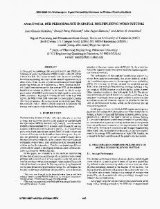
20 18
Capacity [bit per tunnel use]
where h = |h1,1 |2 . In contrast to (10) the capacity does not degrade with increasing L (the number of hops). Since ergodic signaling at every DF node allows to be robust against deep channel fades the capacity is not determined by the weakest channel link. In the large-relay limit we have
16 14 12 10
Non−interfering DF−MPT Non−interfering DF−MPT norm. Interfering DF−MPT (upper bound) Interfering DF−MPT (sim.) AF−MIMO tunnel (sim.)
8 6 4 2 0 0
5
10
15
20
25
30
Relays per layer (K)
Fig. 3. Capacity vs. number of relays per layer for AF MIMO transmission (AF-MIMO) and DF multi-path transmission (DF-MPT) with weakest link signaling, L=5
K2 log e. − 2K + 1 We see that in the limit limK→∞ Cerg ≤ log e the ergodic signaling achieves better capacity results than weakest link signaling. Due to convexity properties of the min{·} operator and by the use of Jensen’s inequality it follows that in general: · ¸ X K K X min {E [Cerg,l ]} = Cerg . E min {CWL,l } ≤ CWL =
of the orthogonal (interference-free) multi-path transmission DF-MPT and clearly outperforms the this scheme for DFMPT norm. The MIMO tunnel achieves much higher capacity results than DF-MPT when interference between the network routes occurs. The reason for the large degradation of the non-orthogonal multi-path transmission here is our simplified interference model, where each interfering signal is in the average equally strong as the desired signal. Note that the interference from the network paths helps us in the MIMO tunnel to establish a rich scattering environment (“good interference”) which is necessary to obtain significant spatial multiplexing gains, whereas the interference in the multi-path transmission approach limits this signaling scheme strongly (“bad interference”). In Fig. 4 we compare the two schemes with respect to the number of hops. The capacity decrease of the MIMO tunnel with respect to the number of hops is due to noise accumulation and the fact that a product of Gaussian matrices becomes increasingly ill-conditioned as the number of concatenated matrices grows. In the multi-path transmission approach every additional hop increases the probability of a weaker link in a path and therefore the probability that the path capacity will be smaller by adding a new link (hop) increases. In Fig. 5 we compare the two schemes when ergodic signaling is used for multi-path transmission. The capacity vs. number of relays behaves qualitatively similar as for weakest link signaling with the difference that the rates are higher for ergodic signaling as (14) suggests.
V. N UMERICAL E XAMPLES
VI. C ONCLUSIONS
We give numerical examples of the capacity performance both for the MIMO tunnel and the multi-path transmission scheme. In Fig. 3 the curve labeled with non-interfering DF-MPT (decode-and-forward multi-path transmission) corresponds to the case where in each layer the average transmit energy per symbol period is equal to Es and the curve labeled with non-interfering DF-MPT norm. corresponds to the case where the capacity is normalized to the number of orthogonal channels K but the average transmit energy per layer is KEs . We observe that the average capacity CAF = E [IAF ] of the MIMO tunnel approaches almost the average capacity
We provided a capacity comparison between the MIMO tunnel with AF relays and the multi-path transmission with DF relays for a weakest link signaling scheme and an ergodic signaling scheme. In the AF case (MIMO tunnel) the interference is desired (“good interference”) and is needed to obtain spatial multiplexing gains. In the DF case (multipath transmission) the interference limits strongly the performance (“bad interference”). Distributed spatial multiplexing via AF relays outperforms DF multi-path transmission in terms of achievable rates when we normalize the capacity to the number of orthogonal dimensions used for the transmission.
0
where we again make the (l) 2 Es PK i=1 |h σ 2 ≪ K−1 | and where k,i
assumption
that
i6=k
(l)
|h1,1 |2
z = PK
i=2
.
(l)
|h1,i |2
The PDF of Z is given as (see Appendix) fZ (z) = ³
K 1+
K K−1 z
´K .
(13)
The capacity follows by evaluating the integral in (12) with the PDF (13). For K/(K − 1) ≈ 1 we obtain Cerg ≤
k=1
l
K2
k=1
l
(14)
60
18 Non−interfering DF−MPT Non−interfering DF−MPT norm. Interfering DF−MPT (upper bound) Interfering DF−MPT (sim.) AF−MIMO tunnel (sim.)
14
Non−interfering DF−MPT Interfering DF−MPT (sim.) Interfering DF−MPT (upper bound) Non−interfering DF−MPT norm. AF−MIMO tunnel (sim.)
50 Capacity [bit per tunnel use]
Capacity [bit per tunnel use]
16
12 10 8 6 4
40
30
20
10 2 0 0
5
10
15
20
0 0
5
Number of hops (L)
Fig. 4. Capacity vs. number of hops for AF MIMO transmission (AF-MIMO) and DF multi-path transmission (DF-MPT) with weakest link signaling, K=10
Depending on the channel coherence time (slow or fast fading) and delay constraints given by the user either weakest link signaling (“short codes”) or ergodic signaling (“long” codes) may be the better choice. A PPENDIX A. PDF of hmin n o (l) Given that h1,1 are i.i.d. CN (0, ν 2 ) it follows 1≤l≤L n o (l) that |h1,1 |2 are i.i.d. according to ν12 exp(− νh2 ). 1≤l≤L
From order statistics [14] we know that the minimum of L independent and exponentially distributed random variables with mean ν 2 has again a probability density function (PDF) which is exponential with mean ν 2 /L.
B. PDF of Y and Z © (l) ª Define z i.i.d. according to fZ (z) where l PK (l) (l) (l) (l) (l) (l) z = y1 /y2 with y1 = |h1,1 |2 and y2 = i=2 |h1,i |2 . The PDF of Z is determined by Z ∞ fZ (z) = y2 fY1 (y2 z)fY2 (y2 )dy2 0
with
=³
K
K 1 + z K−1
fY1 (y2 z) =
´K
1 y2 z exp(− 2 ) 2 ν ν
and K−1 K
fY2 (y2 ) = 2K−1 Γ(K ×
− 1)
µ
µ
√ν (2)
K −1 y2 K
The PDF of y=
min
2≤l≤L−1
¶2(K−1)
¶K−2
(
(l)
y1
(l)
y2
exp
)
µ
¶ K −1 y . 2 Kν 2
10 15 20 Relays per layer (K)
25
30
Fig. 5. Capacity vs. number of relays per layer for AF MIMO transmission (AF-MIMO) and DF multi-path transmission (DF-MPT) with ergodic signaling, L=5
is then given by [14] L−3
fY (y) = (L − 2) [1 − FZ (y)] fZ (y) ¶(L−2)(1−K)−1 µ K y = K(L − 2) 1 + K −1
for K > 1 and L > 2 and where FZ (z) is the CDF of fZ (z). R EFERENCES [1] K. Negus, A. Stephens, and J. Lansford, “HomeRF: wireless networking for the connected home,” vol. 7, pp. 20–27, Feb. 2000. [2] I. Akyildiz, W. Su, Y. Sankarasubramaniam, and E. Cayirci, “A survey on sensor networks ,” IEEE Commun. Mag., vol. 40, pp. 102–114, Aug. 2002. [3] M. Ilyas, The Handbook of Ad Hoc Wireless Networks. CRC Press, 2002. [4] P. Gupta and P. Kumar, “The Capacity of Wireless Networks,” IEEE Trans. Inform. Theory, vol. 46, Mar. 2000. [5] I. E. Telatar, “Capacity of multi-antenna Gaussian channels,” tech. rep., AT&T Bell Laboratories, 1995. [6] G. J. Foschini, “Layered space-time architecture for wireless communication in a fading environment when using multi-element antennas,” Bell Labs Tech. J., vol. 1, pp. 41–59, Autumn 1996. [7] S. Borade, L. Zheng, and R. Gallager, “Maximizing Degrees of Freedom in Wireless Networks,” in Proc. Allerton Conf. Comm., Contr. and Comp., Oct. 2003. [8] M. Dohler, A. Gkelias, and H. Aghvami, “A Resource Allocation Strategy for Distributed MIMO Multi-Hop Communication Systems,” IEEE Commun. Lett., vol. 8, pp. 99–101, Feb. 2004. [9] L. Ozarow, S. Shamai (Shitz), and A. Wyner, “Information theoretic considerations for cellular mobile radio,” IEEE Trans. Veh. Technol., vol. 43, pp. 359–378, May 1994. [10] A. Paulraj, R. Nabar, and D. Gore, Introduction to Space-Time Wireless Communications. Cambridge University Press, 2003. [11] E. Biglieri, J. Proakis, and S. Shamai, “Fading Channels: InformationTheoretic and Communications Apects,” IEEE Trans. Inform. Theory, vol. 44, pp. 2619–2692, Oct. 1998. [12] R. M¨uller, “On the asymptotic eigenvalue distribution of concatenated vector-valued fading channels,” IEEE Trans. Inform. Theory, vol. 48, pp. 2086–2091, July 2002. [13] M. Abramovitz and I. Stegun, Handbook of Mathematical Functions. Dover Publications, Inc., New York, 1972. [14] A. Papoulis and S. U. Pillai, Probability, Random Variables and Stochastic Processes. McGraw-Hill, 4th ed., 2002.