Distributed Testing with Zero-Rate Compression. Wenwen Zhao and Lifeng Lai. Department of Electrical and Computer Engineering. Worcester Polytechnic ...
Distributed Testing with Zero-Rate Compression Wenwen Zhao and Lifeng Lai Department of Electrical and Computer Engineering Worcester Polytechnic Institute {wzhao3, llai}@wpi.edu Abstract—Motivated by distributed inference over big datasets problems, we study multi-terminal distributed hypothesis testing problems in which each terminal has data related to only one random variable. We consider a case of practical interest in which each terminal is allowed to send zero-rate messages to a decision maker. Subject to a constraint that the error exponent of the type 1 error probability is larger than a certain level, we characterize the best error exponent of the type 2 error probability using basic properties of the r-divergent sequences. Index Terms—Distributed testing, error exponent, exponentialtype constraint, zero-rate compression.
I. I NTRODUCTION Inferring the relationship among multiple random variables from data plays an important role in machine learning and statistical inference. The centralized setting in which all of the data is available at one terminal is well studied. Recently, as large-scale datasets are increasingly common, the distributed setting, in which available data is stored in multiple terminals with limited communication channels between them, has attracted significant research interests [1]–[3]. There are two main scenarios for the distributed setting. In the first scenario, each terminal has local data that are related to all of the random variables [2], [3]. Even though each terminal has less data than the centralized setting, it can still perform statistical inference or learning algorithms on its local data. Clearly communications among these terminals can improve the performance. There have been some recent interesting work [1], [2] that characterized the fundamental limits of inference algorithms with communication constraints under this setup. In the second scenario, each terminal has data related to a subset but not all of the random variables. This setup is more challenging than the first scenario, as data exchange among multiple terminals is essential. For example, suppose terminal X1 has data related to random variable X1 , and terminal X2 has data related to random variable X2 , then they have to exchange information to estimate the joint distribution of X1 and X2 . In this paper, we study statistical inference problems for the second scenario from information theory perspective. In particular, we consider a setup with L terminals Xi , i = 1, · · · , L, where terminal Xi has data related to random variable Xi only. These terminals can send information related to their own data using a limited rate to a decision maker Y, which then The work of W. Zhao and L. Lai was supported by the Qatar National Research Fund under Grant QNRF-6-1326-2-532.
978-1-4673-7704-1/15/$31.00 ©2015 IEEE
performs statistical inference based on messages received from these terminals and its own data related to Y . In this paper, we focus on a basic inference problem in which the terminal Y tries to determine the joint probability mass function (PMF) of the data from the following two hypotheses: H0 : PX1 ···XL Y vs H1 : QX1 ···XL Y . We note that in this setup, the decision maker is not required to recover the data of terminals Xi . Instead, it is only required to make a decision regarding which hypothesis is true. This paper builds upon our recent work [4], in which we studied a special case with QX1 ···XL Y = PX1 ···XL PY , i.e., testing against independence case, under a constant-type type 1 error probability constraint (i.e., the type 1 error probability is required to be less than a given constant) and non-zero communication rate constraints. In this paper, we generalize our work [4] by imposing more strict constraints. In particular, we consider the problem with the general form of PMF, i.e., QX1 ···XL Y is not limited to be PX1 ···XL PY anymore. In addition, we impose an exponential-type constraint on the type 1 error probability (i.e., the type 1 error probability is required to decrease exponentially fast with a certain error exponent). Furthermore, we focus on the zero-rate compression case in which each terminal is only allowed to send messages to the decision maker with a diminishing rate (zero-rate compression). If the decision maker were required to fully recover data of terminals Xi s as in the distributed source coding problems [5], [6], this zero-rate compression is not enough. However, in our setup, this zero-rate compression will still be valuable for the decision maker for statistical inference. A clear benefit of this zero-rate compression approach is that the terminals only need to consume a limited amount of communication resources. We fully characterize the best achievable error exponent of the type 2 error probability under these zero-rate compression and the exponential-type type 1 error probability constraints by providing matching lower and upper bounds. Our work is related to several existing interesting work [7]– [12] that lie in the intersection of statistics and information theory. Of particular relevance, among other contributions, [8], [9] considered a similar setup with the exponentialtype constraint on the type 1 error probability and zero-rate constraint on the communication. [8] provided a lower bound on the type-2 error exponent. Later [9] established an upper bound that coincides with the lower bound derived in [8]
2792
ISIT 2015
by converting the exponential-type constraint problems to the constant-type constraint problems considered in [7]. The key difference between the model considered in [8], [9] and our model is that [8], [9] focused on the case where (X1 , · · · , XL ) are all at one terminal, while in our model these random variables are all at different terminals. The remainder of the paper is organized as follows. In Section II, we introduce the model studied in this paper. In Section III, we summarize several fundamental properties of r-divergent sequences that play a key role in the proof. In Sections IV and V, we present our main results. Finally, we offer some concluding remarks in Section VI.
with rate constraint: 1 log Mi ≤ Ri + η, i = 1, · · · , L. (3) n Here, η > 0 is an arbitrarily prescribed number. Using the messages fi (Xin ), i = 1, · · · , L and its side information Y n , the decision maker will use the decision function ψ to determine which hypothesis is true: ψ : M1 · · · ML Y n → {H0 , H1 }.
(4)
For any given decision function ψ, one can define the acceptance region as An = {(X1n , · · · , XLn , Y n ) ∈ X1n × · · · × XLn × Y n :
II. M ODEL
ψ(f1 (X1n ) · · · fL (XLn )Y n ) = H0 }.
Consider random variables (X1 , · · · , XL , Y ) taking values in a finite set X1 × · · · × XL × Y and admitting a joint PMF that has two possible forms:
For any given fi , i = 1, · · · , L and ψ, the type 1 error n (Acn ) and the type 2 probability is defined as αn = PX 1 ···XL Y n error probability is defined as βn = QX1 ···XL Y (An ). Our goal is to design the encoding functions fi and the decision function ψ to maximize the type 2 error exponent under the constraint that the type 1 error exponent is larger than a given level and the communication rate constraints (3). More specifically, for a given r > 0, we require
H0 : PX1 ···XL Y
or
H1 : QX1 ···XL Y .
(1)
(X1n , · · · , XLn , Y n ) are independently and identically generated according to one of the above joint PMFs. In a typical hypothesis testing problem, one determines which hypothesis is true under the assumption that (X1n , · · · , XLn , Y n ) are fully available at the decision maker. In this paper, we consider a setting in which Xin , i = 1, · · · , L and Y n are at different terminals. In particular, terminal Xi observes only Xin and terminal Y observes only Y n . Terminals Xi s are allowed to send messages to terminal Y. Using Y n and the received messages, terminal Y determines which hypothesis is true. We denote this system as SX1 ···XL |Y . Figure 1 illustrates the system model. In the following, we will use the term “decision maker” and terminal Y interchangeably. Here, Y n is used to model any side information available at the decision maker. If Y is set to be the empty set, then the decision maker does not have side information. We note that the model here is different from the traditional distributed source coding with side information problems [5], [6] whose goal is to fully recover (X1n , · · · , XLn ) at terminal Y.
αn ≤ exp(−nr),
in which the maximization is over all f1 , · · · , fL , ψ satisfying conditions (3) and (6). With these notation, our goal mentioned above is then to characterize σ(R1 , · · · , RL , r) , lim σ(R1 , · · · , RL , r, η). η↓0
More specifically, the system consists of L encoders fi , i = 1, · · · , L, one at each terminal Xi , and one decision function ψ at the decision maker Y. After observing the data sequence xni ∈ Xin , encoder fi transforms the sequence xni into a message fi (xni ) taking values from the message set Mi fi : Xin → Mi = {1, 2, . . . , Mi },
(2)
(8)
A special case of the model described above is the case with “zero-rate” compression, in which Mi → ∞, as n → ∞,
(9)
1 log Mi → 0, i = 1, · · · , L. (10) n In this case, σ(R1 , · · · , RL , r) is denoted as σ(+0, · · · , +0, r). It is well-known that in the traditional distributed source coding with side information problems [5], [6], in which the goal is to recover (X1n , · · · , XLn ) at terminal Y, this zero-rate information will not be useful. However, in our setup, the goal is only to determine which hypothesis is true. This zero-rate information will be very useful. Our model is related to but different from several existing interesting work [4], [7]–[9], [11]. The first class of existing work, such as [8] and [9], considered the case with only one encoder that has full access to (X1n , · · · , XLn ) (which can then be viewed as a single super-variable X n = (X1n , · · · , XLn )), while in our model each of the L encoders has access to only Ri =
Model
(6)
which implies that the type 1 error probability must decease exponentially fast with an exponent no less than r. Also, define ( ) 1 σ(R1 , · · · , RL , r, η) = max lim inf − log βn , (7) f1 ,··· ,fL ,ψ n→∞ n
but
Fig. 1.
(5)
2793
partial information. The second class of existing work, such as [4], [7], [11], considered the case with a less strict type 1 error probability constraint than (6). In particular, [4], [7], [11] studied a constant-type constraint in which one requires αn ≤ ϵ,
(11)
for a given constant ϵ. In the following, we will use θ(R1 , · · · , RL , ϵ) to denote the best type 2 error exponent under the constant-type type 1 error constraint (11). III. r-D IVERGENT S EQUENCES
on the error exponent using the results in [7] for the constanttype constraint. Here the positivity condition QX1 X2 Y > 0 is needed to invoke “Blowing up lemma” [13] in the proof of in [7]. Theorem 1. Let PX1 X2 Y be arbitrary and QX1 X2 Y > 0. For zero-rate compression in SX1 X2 |Y with R1 = R2 = +0, the error exponent satisfies σ(+0, +0, r) ≤ σopt ,
(14)
in which
The concept of r-divergent sequences plays an important role in the following sections. In this section, we review the definition and some important properties of r-divergent sequences. More details and properties of r-divergent sequences can be found in [8]. In this paper, we use tp(xn ) to denote the type of any nsequence xn = (x1 , · · · , xn ) ∈ X n . Furthermore, we call a random variable X (n) that has the same distribution as tp(xn ) as the type variable of xn .
σopt ,
min
P˜X1 X2 Y ∈Hr
D(P˜X1 X2 Y ||QX1 X2 Y )
with
{ Hr = P˜X1 X2 Y : P˜X1 = PˆX1 , P˜X2 = PˆX2 , P˜Y = PˆY } for some PˆX1 X2 Y ∈ φr , (16) φr = {PˆX1 X2 Y : D(PˆX1 X2 Y ||PX1 X2 Y ) ≤ r}.
Definition 1. ( [8]) Let X be a random variable taking values in a finite set X with PMF PX , and r ≥ 0. An n-sequence xn = (x1 , . . . , xn ) ∈ X n is called r-divergent sequence for X if D(X (n) ||X) ≤ r, (12)
where
where X (n) is the type variable of xn . The set of all rdivergent sequences is denoted by Srn (X).
Equations (18) and (19) imply that
In particular, S0n (X) (i.e., r = 0) represents the set of all x sequences such that tp(xn ) = PX . The following lemma from [8] summarizes key properties of r-divergent sequences.
(15)
(17)
Proof: Let An be an arbitrary acceptance region such that αn ≤ exp(−nr),
r>0
n (Acn ). αn = PX 1 X2 Y
n (An ) ≥ 1 − exp(−n(r − γ)) ∀n ≥ n0 PX 1 X2 Y
(18) (19)
(20)
n
Lemma 1. ( [8]) Let r > 0 be fixed. 1) Pr{X n ∈ Srn (X)} ≥ 1 − (n + 1)|X | · exp(−nr). 2) Let An be a subset of X n and n PX (An ) ≥ 1 − exp(−nr)
holds. Let An (X |An (X
(n)
(n)
(
) , An ∩
S0n (X (n) ),
)| ≥ 1 − (n + 1)
|X |
where γ > 0 is an arbitrarily small constant. Next, select an arbitrary “internal point” PX10 X20 Y0 ∈ φr , where φr is specified in (17). Then clearly D(PX10 X20 Y0 ||PX1 X2 Y ) < r.
(21)
Define (13)
Tˆn (δ) = {joint types Pˆn on X1n × X2n × Y n : D(Pˆn ||PX10 X20 Y0 ) < δ} (22)
we have
) · exp[−n(r − cn )]
where δ > 0 is an arbitrary constant. Then, in view of (21) and the uniform continuity of the divergence, for all Pˆn ∈ Tˆn (δ) it holds that
|S0n·(X (n) )| in which cn = D(X (n) ||X).
cn ≡ D(Pˆn ||PX1 X2 Y ) < r − 2γ,
IV. T HE C ASE WITH L = 2 In this section, to assist the presentation, we focus on the case with L = 2 and provide details on how to characterize σ(+0, +0, r). We will discuss the general case in Section V.
(23)
provided that we take γ > 0 and δ > 0 sufficiently small. Consequently, according to Lemma 1, we have |An (Pˆn )| ≥ (1 − (n + 1)|X1 ||X2 ||Y| exp(−nr))|S0 (Pˆn )| (24) for all Pˆn ∈ Tˆn (δ). Now we define the set
A. Converse We first establish an upper bound on the error exponent that any scheme can achieve. We will follow the similar strategy as in [9]. In particular, we will first convert a problem with the exponential-type constraint to a corresponding problem with the constant-type constraint. We then obtain an upper bound
Tn (δ) = {(xn1 , xn2 , y n ) ∈ X1n × X2n × Y n : (n) (n) X X Y (n) ∈ Tˆn (δ)} 1
2
(25)
and consider an i.i.d. random sequence of length n generated according to the probability distribution PX10 X20 Y0 . Then,
2794
When Y n is not fully available to the decision maker, all of the X1 , X2 , Y terminals will compress their observations and send messages at rates R1 , R2 and R, respectively, to the decision maker who will then determine which hypothesis is true. We denote this system as SX1 X2 Y . We will also use σ(R1 , R2 , R, r) to denote the largest error exponent of the type 2 error under the rate constraint and the constraint that the error exponent of the type 1 error probability is no less than r. Clearly, setting R ≥ log |Y|, we recover the case when Y n is fully observable at the decision maker. If all of the three terminals send messages using zero-rate compression, then the error exponent is σ(+0, +0, +0, r). In the following, we show σ(+0, +0, +0, r) is no less than σopt defined in (15).
from (24), we have n n PX (An ) ≥ PX (An ∩ Tn (δ)) 10 X20 Y0 10 X20 Y0 ∑ n = PX (An ∩ S0 (Pˆn )) 10 X20 Y0 Pˆn ∈Tˆn (δ)
∑
=
n PX (An (Pˆn )) 10 X20 Y0
Pˆn ∈Tˆn (δ)
≥ (1 − (n + 1)|X1 ||X2 ||Y| exp(−nr)) ∑ n · PX (S0 (Pˆn )) 10 X20 Y0 Pˆn ∈Tˆn (δ)
= (1 − (n + 1)|X1 ||X2 ||Y| exp(−nr)) PX (n) X (n) Y (n) (Tˆn (δ)) 10
20
0
≥ (1 − (n + 1)|X1 ||X2 ||Y| exp(−nr)) ·(1 − (n + 1)|X1 ||X2 ||Y| exp(−nδ)). (26) Now consider the zero-rate (R1 = +0, R2 = +0, R ≥ 0) hypothesis testing problem with H0 : PX10 X20 Y0
vs H1 : QX1 X2 Y .
Theorem 2. For zero-rate compression in SX1 X2 Y with R1 = R2 = R = +0, the error exponent satisfies σ(+0, +0, +0, r) ≥ σopt where σopt is defined as (15). Proof: First, set
(27)
˜1, X ˜ 2 , Y˜ ) = f (X
Then, for this hypothesis testing problem, if we use the same acceptance region An as above, the type 1 error probability n (An ) αn(0) = 1 − PX 10 X20 Y0
≤ 1 − (1 − (n + 1)|X1 ||X2 ||Y| exp(−nr)) ·(1 − (n + 1)|X1 ||X2 ||Y| exp(−nδ)) ≤ ϵ. Hence, for the hypothesis testing problem (27), the acceptance region An satisfies the constant-type type 1 error probability constraint. From [7], we know that the type 2 error exponent θ(+0, +0, ϵ) ≤
min
P˜X1 X2 Y ∈L0
D(P˜X1 X2 Y ||QX1 X2 Y ),
(28)
min
PˆX1 X2 Y PˆX1 = P˜X1 PˆX2 = P˜X2 PˆY = P˜Y
D(PˆX1 X2 Y ||PX1 X2 Y )
which is continuous in ((P˜X1 )x1 ∈X1 , (P˜X2 )x2 ∈X2 , (P˜Y )y∈Y ). Next, divide the (|X1 | + |X2 | + |Y|) dimensional unit cube into equal-sized M1 · M2 · M small cells with each edge of length κ1 along the first |X1 | components, each edge of length κ2 along the |X2 | components and each edge of length τ along the |Y| components, where −1/|X1 |
κ1 = M1
,
−1/|X2 |
κ2 = M2
,
τ = M −1/|Y| ,
in which M1 → ∞, M2 → ∞, M → ∞,
where L0 = {P˜X1 X2 Y : P˜X1 = PX10 , P˜X2 = PX20 , P˜Y = PY0 }. On the other hand, we note that PX10 X20 Y0 was arbitrary as far as condition (21) is satisfied. Therefore, in the light of the definition of Hr , we see that the infimum of the right-hand side in (28) over all possible internal points PX10 X20 Y0 satisfying (21) coincides with min
P˜X1 X2 Y ∈Hr
D(P˜X1 X2 Y ||QX1 X2 Y ).
Thus (28) reduces to σ(+0, +0, r) ≤
min
P˜X1 X2 Y ∈Hr
D(P˜X1 X2 Y ||QX1 X2 Y ).
B. Achievability In this subsection, we show that the error exponent characterized in the converse can be achieved even if the decision maker does not have full observation about Y n .
(29)
(30)
but log Mi /n → 0 for i = 1, 2 and log M/n → 0, as n → ∞ (i.e., zero-rate compression for all three terminals). Choose and fix a representative point in each cell for ˜1, X ˜ 2 , Y˜ ). Then in a given cell, we every set of variables (X ˇ1, X ˇ 2 , Yˇ ) correspond make its representative variable set (X ˇ ˇ in such a way that((PX1 )x1 ∈X1 , (PX2 )x2 ∈X2 , (PˇY )y∈Y ) is the representative point of ((P˜X1 )x1 ∈X1 , (P˜X2 )x2 ∈X2 , (P˜Y )y∈Y ). For each terminal, after observing its sequence, determines its type and then finds the index of the corresponding edge. Each terminal then sends the index to the decision maker. After receiving all the indexes, the decision maker can determine the cell index. Since we have assumed (30), we see that with any η > 0 |P˜X1 − PˇX1 | < η, x1 ∈ X1 , |P˜X2 − PˇX2 | < η, x2 ∈ X2 , |P˜Y − PˇY | < η, y ∈ Y,
(31) (32) (33)
for sufficiently large n ≥ n0 (η). Furthermore, the continuity
2795
˜1, X ˜ 2 , Y˜ ) in (X ˜1, X ˜ 2 , Y˜ ) yields of f (X ˜1, X ˜ 2 , Y˜ ) − f (X ˇ1, X ˇ 2 , Yˇ )| < η. |f (X
(34)
ˇ (n) , X ˇ (n) , Yˇ (n) ) the representative point of Denoting by (X 1 2 (n) (n) (n) (n) (n) (X1 , X2 , Y ) where X1 , X2 and Y (n) are the type n n n n variables of x1 ∈ X2 , x2 ∈ X2 and y n ∈ Y n respectively, we set an acceptance region (n)
V. G ENERAL C ASE The results of the previous section can be extended to the general case with L terminals. We have the following theorem. Theorem 4. Let PX1 ,··· ,XL Y be arbitrary and QX1 ,··· ,XL Y > 0. For zero-rate compression in SX1 ···XL |Y with Ri = +0, i = 1, · · · , L and type 1 error constraint (6), the best type 2 error exponent
(n)
ˇ ,X ˇ , Yˇ (n) ) ≤ r + 2η}. An = {(xn1 , xn2 , y n ) : f (X 1 2
σ(+0, · · · , +0, r) =
For any ρ > 0 set ξρ = {(xn1 , xn2 , y n ) :
(n) (n) f (X1 , X2 , Y (n) )
≤ ρ};
where
then in view of (34) it is clear that ξr+η ⊂ An ⊂ ξr+3η It is easy to see that (xn1 , xn2 , y n ) ∈ n n Sr+η (X1 X2 Y ), that is Sr+η (X1 X2 Y
(35)
ξr+η if ∈ ) ⊂ ξr+η , which yields
for n large enough. Hence, the constraint (6) is satisfied. On the other hand, from the second inclusion in (35), βn = QnX1 X2 Y (An ) ≤ QnX1 X2 Y (ξr+3η ) ∑ ≤ (n)
(n)
(n)
exp(−nD(X1 X2 Y (n) ||QX1 X2 Y ))
≤ (n + 1)|X1 ||X2 ||Y| ·
(n)
max (n) (n) X1 X2 Y (n) (n) (n) f (X1 , X2 , Y (n) ) ≤
(n)
exp(−nD(X1 X2 Y (n) ||QX1 X2 Y ) r + 3η
|X1 ||X2 ||Y|
≤ (n + 1) [ { · exp − n
˜1X ˜ 2 Y˜ ||QX X Y ) D(X 1 2
min
˜1 X ˜ 2 Y˜ X ˜1 , X ˜ 2 , Y˜ ) ≤ r + 3η f (X
}] .
Therefore, σ(+0, +0, +0, r) ≥
min
P˜X1 X2 Y ∈Hr+3η
D(P˜X1 X2 Y ||QX1 X2 Y ),
which establishes (2) if we let η → 0. As σ(+0, +0, r) = σ(+0, +0, log |Y|, r). From Theorem 2, we have σ(+0, +0, r) = σ(+0, +0, log |Y|, r) ≥ σ(+0, +0, +0, r) ≥ σopt . Coupled with Theorem 1, we have: Theorem 3. Let PX1 X2 Y be arbitrary and QX1 X2 Y > 0. For zero-rate compression in SX1 X2 |Y with R1 = R2 = +0 and type 1 error constraint (6), the best type 2 error exponent σ(+0, +0, r) = σopt . where σopt is defined as (15).
(36)
(37)
{ Hr = P˜X1 ···XL Y : P˜Xi = PˆXi ,
φr = {PˆX1 ···XL Y : D(PˆX1 ···XL Y ||PX1 ···XL Y ) ≤ r}.
(39)
VI. C ONCLUSION In this paper, we have discussed distributed inference problems under the zero-rate compression and exponentialtype type 1 error probability constraints. Using properties of r-divergence sequences, we have characterized the best error exponent of the type 2 error probability. We have also generalized to the case with an arbitrary number of terminals. R EFERENCES
(n)
X1 X2 Y (n) (n) (n) f (X1 , X2 , Y (n) ) ≤ r + 3η
D(P˜X1 ···XL Y ||QX1 ···XL Y )
i = 1, · · · , L } for some PˆX1 ···XL Y ∈ φr , (38)
(xn1 , xn2 , y n )
n 1 − αn = PX (An ) ≥ 1 − exp(−nr) 1 X2 Y
min
P˜X1 ···XL Y ∈Hr
[1] M.-F. Balcan, A. Blum, S. Fine, and Y. Mansour, “Distributed learning, communication complexity and privacy,” ArXiv e-prints, Apr. 2012. [2] Y. Zhang, J. C. Duchi, M. I. Jordan, and M. J. Wainwright, “Informationtheoretic lower bounds for distributed statistical estimation with communication constraints,” Advances in Neural Information Processing Systems 26, pp. 2328–2336, 2013. [3] O. Shamir and N. Srebro, “Distributed stochastic optimization and learning,” in Proc. Allerton Conf. on Communication, Control, and Computing, (Montecello, IL), Oct 2014. [4] W. Zhao and L. Lai, “Distributed testing against independence with multiple terminals,” in Proc. Allerton Conf. on Communication, Control, and Computing, (Montecello, IL), pp. 1246–1251, Oct 2014. [5] D. Slepian and J. Wolf, “Noiseless coding of correlated information sources,” IEEE Trans. Inform. Theory, vol. 19, pp. 471–480, July 1973. [6] A. El Gamal and Y.-H. Kim, Network Information Theory. Cambridge, UK: Cambridge Unversity Press, 2012. [7] H. Shalaby and A. Papamarcou, “Multiterminal detection with zero-rate data compression,” IEEE Trans. Inform. Theory, vol. 38, pp. 254–267, March 1992. [8] T. S. Han and K. Kobayashi, “Exponential-type error probabilities for multiterminal hypothesis testing,” IEEE Trans. Inform. Theory, vol. 35, pp. 2–14, Jan 1989. [9] T. S. Han and S.-I. Amari, “Statistical inference under multiterminal data compression,” IEEE Trans. Inform. Theory, vol. 44, pp. 2300–2324, Oct 1998. [10] C. Tian and J. Chen, “Successive refinement for hypothesis testing and lossless one-helper problem,” IEEE Trans. Inform. Theory, vol. 54, pp. 4666–4681, Oct. 2008. [11] M. S. Rahman and A. B. Wagner, “The optimality of binning for distributed hypothesis testing,” IEEE Trans. Inform. Theory, vol. 58, pp. 6282–6303, Oct. 2012. [12] Y. Xiang and Y.-H. Kim, “Interactive hypothesis testing against independence,” in Proc. IEEE Intl. Symposium on Inform. Theory, (Istanbul, Turkey), pp. 2840–2844, July 2013. [13] R. Ahlswede, P. G´acs, and J. K¨orner, “Bounds on conditional probabilities with applications in multi-user communication,” Zeitschrift f¨ ur Wahrscheinlichkeitstheorie und Verwandte Gebiete, vol. 34, no. 2, pp. 157–177, 1976.
2796