Approaching Optimal Compression with Fast Update for Large Scale Routing Tables Tong Yang, Bo Yuan, Shenjiang Zhang, Ting Zhang, Ruian Duan, Yi Wang, and Bin Liu* Tsinghua National Laboratory for Information Science and Technology Department of Computer Science and Technology, Tsinghua University, Beijing, China Abstract—With the fast development of Internet, the size of routing tables in the backbone routers keeps a rapid growth in recent years. An effective solution to control the memory occupation of the ever-increased huge routing table is the Forwarding Information Base (FIB) compression. Existing optimal FIB compression algorithm ORTC suffers from high computational complexity and poor update performance, due to the loss of essential structure information during its compression process. To address this problem, we present two sub-optimal FIB compression algorithms -- EAR-fast and EAR-slow, respectively, based on our proposed Election and Representative (EAR) algorithm which is an optimal FIB compression algorithm. The two suboptimal algorithms preserve the structure information, and support fast incremental updates while reducing computational complexity. Experiments on an 18month real data set show that compared with ORTC, the proposed EAR-fast algorithm requires only 9.8% compression time and 37.7% memory space, but supports faster update while prolonging the recompression interval remarkably. All these performance advantages come at a cost of merely a 1.5% loss in compression ratio compared with the theoretical optimal ratio.
I.
INTRODUCTION
Internet has maintained a rapid growth for years, leading to a roughly 15% annual increase of the routing table size [2]. Taking the AS6447 1 as an example, it had only about 70K entries in its routing table in 2000, but went beyond 400K at the beginning of 2012 [3]. Routing tables grow so rapidly that ISPs struggle to keep up with it. For those routers installed years ago, if the designed capacity of the Forwarding Information Base (FIB) is less than the current increased routing table size, ISPs should seek a better compression algorithm to suppress the table growth, so as to postpone the need of replacing their infrastructures in the near future. Making the matter worse, routing updates are also increasing rapidly more than ever before, due to enhanced Internet functionalities in recent years [4]. These make FIB compression an important but challenging issue. In [1], Draves et al. proposed ORTC algorithm to construct an optimal routing table via two basic operations: ‘and’ and ‘union’. Actually, there exists more than one optimal routing table, and we propose Election and Representative (EAR) algorithm to construct a different 2 optimal routing table *Corresponding author:
[email protected]. Others: {yang-t10, yuanb03, zsj09, ting-zhang10, dra08, yiwang09} @mails.tsinghua.edu.cn. Supported by NSFC (61073171, 60873250), Tsinghua University Initiative Scientific Research Program (20121080068), the Specialized Research Fund for the Doctoral Program of Higher Education of China (20100002110051).
978-1-4673-1298-1/12/$31.00 ©2012 IEEE. 1
AS6447 is a backbone router’s autonomous system number. The compressed tries of EAR and ORTC have different structures, but their numbers of solid nodes (prefix number) are equal.
2
through a different approach. Unfortunately, optimal compression algorithms have the following two inherent shortcomings: a) High compression complexity. From a sociological point of view, in order to elect the most popular candidate, all the votes should be recorded and computed. This is obviously time-consuming. The EAR algorithm follows a process similar to the election procedure. Logically, EAR algorithm can be divided into two steps: 1) election – making statistics of the sub-trie nodes’ next-hop and electing the most prevalent one; 2) representative – deleting the winning voters (those nodes which share the same next-hop with the most prevalent nexthop node). Similar to the time-consuming election, EAR suffers from high computational complexity, so does ORTC. b) Poor update performance. Incremental update algorithm operates in the sub-trie using the corresponding compression algorithm. Therefore, complicate compression algorithm incurs complicate incremental update algorithm. In addition, ORTC is not conducive to incremental update, because it does not preserve the structure information3. When designing a compression algorithm, we focus on the following five metrics in the design space: 1) high compression ratio4; 2) short compression time; 3) low memory cost; 4) fast incremental update and; 5) long recompression interval (the interval between two adjacent events of recompressing the whole routing table). The system performance will be optimized, only if all the above metrics are achieved. Unfortunately, ORTC only concentrates on the compression ratio, ignoring the others. In order to cover the five metrics, we present two suboptimal compression algorithms based on our proposed EAR. The idea is originated from the election process as well. In the election process of democratic society, it is usually timeconsuming to elect the most popular candidate, and only a few candidates are likely to be elected as representatives. An effective approach is to directly elect the most ‘promising’ candidate, so as to simplify the election process. Similarly, according to our experimental tests, we discover that EAR and ORTC often consume too much time and memory (inefficient time and memory) only for a little increase in compression ratio. We also find that the ‘promising’ nodes (those nodes with shallow depth, such as node A in Figure 2(c)) are usually elected as representatives. To map the social solution to compression algorithm, we refine EAR into two 3
The details of structure information are illustrated in the second paragraph of the Related Work in this paper. 4 Compression ratio is defined as the ratio of the number of nodes in compressed trie to that of the original trie. For convenience, in this paper, ‘high compression ratio’ stands for a small number of compressed prefixes.
suboptimal compression algorithms, named EAR-slow and EAR-fast, respectively. The two suboptimal algorithms directly select the most promising candidate node as representative, avoiding traversing the sub-trie. Their design philosophy is to simplify the election process by eliminating the ‘inefficient’ time and memory occupation at the cost of sacrificing a very small compression ratio. Furthermore, the EAR-slow and the EAR-fast algorithm preserve the structure information only using an integer variable for each node. As a result, they can achieve a well-balanced trade-off among the above five metrics. Particularly we have the following contributions: •
We propose two sub-optimal algorithms based on EAR: EAR-fast and EAR-slow, which preserve the structure information attached in a single compressed trie to reduce the need for secondary storage5, achieving long recompression interval while approaching the optimal compression ratio. • The proposed incremental update algorithms avoid traversing the sub-trie, thus simplifying the operations, leading to a faster update speed. The remaining parts of this paper are organized as follows. Section II surveys the related work. Section III presents EAR algorithm and its two derived suboptimal compression algorithms. Section IV elaborates on our fast incremental update algorithms. Extensive evaluation and the analysis over a large-scale real data set are conducted in Section V, and finally we conclude this paper in Section VI. II.
RELATED WORK
IRTF RRG [8] and IETF [9] have been working on the routing scalability problem for years. Generally speaking, there are two categories of solutions: the first category is Map-andEncap [10-15], which requires changing the routing architecture and protocols; the second is FIB compression, which is a local solution and needs no change to the existing routing protocols. Our algorithms belong to the latter one and the representative papers in this category are [1], [5-7], [16-17]. Trie-based algorithms are commonly used in FIB compression, given its fast search speed and high update performance [18]. The pioneer effort ORTC [1] worked on the routing table and achieved optimal compression ratio. Its idea is to traverse the entire sub-trie and select the most prevalent next-hop nodes using two operations: ‘and’ and ‘union’. However, traversing the entire sub-trie incurs long time. In addition, ORTC does not preserve the structure information, i.e., the relationships among the original trie nodes, and breaks the original trie structure by creating many new nodes and deleting many existing nodes. Consequently, it leads to probability of some wrong update operation, such as ‘delete a node which does not exist’ and ‘change a node without next hop’. In order to purse the update function, ORTC has to add additional data structures (secondary storage) to help remember the structure information. Therefore, in [5], Yaoqing Liu et al. added incremental update algorithm to ORTC by constructing three additional tries to save the structure information. Coordinating multiple data structures incurs complexity. It is worthy to mention that the source code of ORTC (named as ORTC-Draves in the rest of the paper for easy 5
The details of second storage are illustrated in paragraph 2 of Related Work.
quoting) is inefficient and incomplete, and fails to cover the case of NULL root node. To conduct a fair comparison, we reimplement ORTC algorithm, named ORTC-Perfect, which has both a better compression ratio and a lower computation (CPU and memory) requirement than those of ORTC-Draves. We also find that the update algorithm of ORTC-Draves’, which was implemented in [5] using four tries, consumes too much memory with redundancy and inefficiency, so we re-implement the incremental update algorithm based on ORTC-Perfect using two tries, which is much more efficient and is considered a new version for a more accurate comparison. In [6], Xin Zhao et al. proposed an algorithm (which is called 4-level algorithm in this paper), enabling a flexible choice for users, but it has some shortcomings: 1) the third and the fourth level compression can only deal with non-routable space case. The non-routable packets, which should be dropped given no next-hop found, are forwarded anyway. We call this phenomena roaming garbage in this paper. Our test on real traffic trace shows that the proportion of the roaming garbage traffic could be up to 0.31% and it covers 0.38% of the overall IP address space; 2) the 4-level algorithm probably triggers the ‘routing table fluctuation’ problem, which will be illustrated in Section IV.B.3. In [16], a patent technology (we call it patent algorithm in this paper) proposed a compression algorithm, which is simple and fast, but with poor compression ratio. In [17], the binary trie was changed into the trigeminal trie, which corresponds to the three-state properties of TCAM. Therefore, a better compression ratio might be achieved. However, it is limited to be used in TCAM only, which is an expensive solution. What is worse, the update messages could induce domino effect. Thus the algorithm is difficult to apply, especially in current situation with frequent updates. To gain better compression ratio, Qing Li et al. proposed an algorithm by adopting suboptimal routing [7]. This could potentially cause serious traffic congestion and the update performance is quite questionable. Based on our initial investigation, it can hardly guarantee an O(1) updating complexity [21]. Our work is also based on the trie, but with two major improvements: 1) when manipulating the trie structure for achieving compression, we keep the structure information; 2) we do not traverse the whole trie to get the most prevalent node, but directly elect the most promising one instead, thus saving the compression time. To the best of our knowledge, this is the first effort on balancing a multi-dimensional system optimization for the routing table compression issue and our approach strikes a good trade-off among compression ratio, compression time, memory cost, fast incremental update, as well as recompression interval. III.
COMPRESSION ALGORITHMS
A. Terms and Definitions TABLE I.
TERMS AND DEFINITIONS.
Terms
Definitions
Oldport Newport
the next-hop of a prefix in FIB before compression the next-hop of a prefix in FIB after compression the next-hop of an update message in the operation of insertion and changing the next-hops of a prefix in FIB before and after compression the next-hop of the nearest and non-empty ancestor node before compression the next-hop of the nearest and non-empty ancestor node after compression
Insertport Oldport/Newport Default-oldport Default-newport
The above terms will be used in this paper, and their meanings are given in Table I. As shown in Figure 1, every node has a pair of next-hops: Oldport/Newport. Newport is represented by the shape. For convenience, three next-hops are introduced: solid ellipse, solid rectangle, and solid triangle, representing the Newport of 1, 2, and 3, respectively. For example, the shape of is triangle, pointing its Newport is 3. Oldport is represented by the number in the node (such as 1 in ), and the hollow node (such as ) suggests that its Newport is 0 (There is no prefix in the node after compression). For example, is represented by 1/2, indicating its Oldport is 1, and Newport is 2; is represented by 2/0, indicating its Oldport is 2, and Newport is 0. B. An Example of EAR EAR and its two suboptimal algorithms all follow a process that is similar to the election of a democratic society. Each node has a next-hop, while each candidate has a vote. Actually, any candidate’s next-hop has the opportunity to be selected as representative. All the nodes which share the same next-hop with the representative can be deleted. Therefore, in order to achieve optimal compression (meaning that the compressed routing table has the minimal number of prefixes), the most popular next-hop should be chosen, in other words, should be elected as representative. This is the rationale of EAR.
(a) trie I
(b) trie II
(c) trie III
(d) trie IV
Figure 1. An example of EAR.
We give an intuitive example for the EAR algorithm in Figure 1. Figure 1(a) is original trie, and Figure 1(b) is the trie after leaf-pushing (this technique was proposed by Srinivasan et al. in [19]), which is a preparation of election; Figure 1(c) is the trie after representative, and Figure 1(d) is the trie after representative, which is also the ultimate result of EAR. In contrast, traditional algorithms (such as ORTC, 4-level) do not preserve Oldport and the hollow leaf nodes (such as B and D in Figure 1(d)), causing missing structure information. Election: Node A, B, C, and D are four ‘candidate’ nodes, participating in election. Obviously, hop 2 (rectangle B and D) should be elected as representative, thus node E is set to 1/2. Representative: Node E executes its right of representative: set the Newport of its supporters (node B and D) to 0. It means that node B and D are set to 2/0. In other words, the Newport of the winning voters (node B and D) is set to 0. In this example, the original prefix number is 5 (only the solid nodes are needed to be counted6), and the compressed prefix number is 3, thus the compression ratio is 3/5. This is the process of Election And Representative (EAR). Different from traditional algorithms, EAR completely preserves the trie structure information using Oldport/Newport. The overhead is just an integer for each node, which is very small. The significance of trie structure information is highlighted during the update process. For instance, given an 6
Because the routing table size usually means the prefix number, which is equal to the solid node number in the Trie.
update message: withdraw 11* (see Figure 1), it means node D should be deleted. However, traditional algorithms will find that D does not exist. To guarantee the correctness of update, additional complicate work should be finished, such as a serial of operations in the original trie. In contrast, EAR just needs to set D to 0/1, remarkably reducing time and space. C. Compression Algorithm EAR and its two suboptimal algorithms all consist of two basic operations, named ‘election’ and ‘representative’. 1) Election and Representative ‘Representative’ operation is executed after a successful ‘election’ operation. Those nodes participating in elections, must satisfy the following requirements: they must be 1) solid and hollow; 2) siblings (if a node has no sibling node, a substitute must be created with the next-hop of 0/Defaultoldport); 3) elected representatives (if not, the point must be traced to a leaf node in the sub-trie rooted at the unelected node, then recursive election should be done step by step). Election: Two or more nodes elect their common ancestor node, under the constraint that no solid node appears in the path from the candidate nodes to their common ancestor node. The most prevalent next-hop will be elected as representative, and the common ancestor’s next-hop will be replaced by the most prevalent next-hop. If there is more than one prevalent next-hop, election fails. In this case, the common ancestor’s next-hop will be set to 0, and then the common ancestor will participate in the next round of election. Representative: After a successful election, the common ancestor will exercise the right of being a representative: the Newport of its supporters (those candidates which share the same next-hop with the representative’s) is set to 0. In other words, after representative, the Newport of all the winning voters will be set to 0. 2) Atomic Equivalent Models of EAR Algorithm TABLE II.
NODE’S ATTRIBUTES.
single-node attributes (Category 1) the first attribute solid
hollow
the second attribute has got no brother brother
two-node attributes (Category 2) share the same hop
with different hops
As shown in Table II, in order to cover all the possible situations, candidate nodes’ attributes are classified into two categories. According to these attributes, all atomic election models can be enumerated. Category 1: Single-node election. In this case, a candidate node has no brother. If the node is solid, model 1 emerges. If the node is hollow, model 2 emerges. Model 1: As shown in Figure 2(a), node A has no brother. According to the requirements of the election, at least two nodes are needed, so node B is created with 0/Default-oldport. Model 2: As shown in Figure 2(b), the election and representative process is similar to model 1. Category 2: According to the two-node attributes, four models emerge. Model 3: As shown in Figure 2(c), A is solid and B is hollow. Node A and the sub-trie rooted at node B participate in the election. The most prevalent next-hop will be elected.
Model 4: As shown in Figure 2(d), both A and B are hollow. The two sub-tries rooted at node A and B participate in the election. As same as Model 3, the most prevalent next-hop will be elected. Model 5: As shown in Figure 2(e), both A and B are solid, and have the same Newport, so the common Newport is elected as the Newport of node C. Model 6: As shown in Figure 2(f), both A and B are solid, but have different Newports. In this case, just set C’s Newport to 0.
(a) Model 1
(d) Model 4
(b) Model 2
(e) Model 5
(c) Model 3
(f) Model 6
Figure 2. EAR’s atomic equivalent models.
These six models have covered all the election situations. In order to achieve optimal, a second election should be conducted to elect any one of the most prevalent next-hop for the failed election. In this way, a trie can be compressed into an optimal one. 3) Atomic Equivalent Models of EAR-slow Algorithm As mentioned above, we refine EAR to EAR-slow and EAR-fast, respectively, by directly electing the most promising candidate node, so as to reduce the computational complexity. EAR-slow is a bridge to EAR-fast, and experimental results show that its sacrificed compression ratio is only 0.7%, compared with ORTC-Perfect. The differences between EAR and EAR-slow lie in Model 3 and Model 4. Let us focus on the Model 3 in Figure 2. The two models include the sub-trie rooted at B, thus this election costs too much time. However, there are only two election results: A is elected or no node is elected. Therefore, Model 3 is changed into Model 3’ (see Figure 3(a)): if the Newport of A does not appear in the sub-trie rooted at B, election fails and node C is set as Oldport/0; otherwise, node C’s Newport is set to A’s Newport.
(a) Model 3’
additional nodes, wasting too much time, and breaking the trie structure. The rationale of EAR-fast is to keep the original trie structure unchanged during compression based on EAR-slow. In this way, no node is needed to be created, so as to accelerate compression and support fast incremental update. The cost is merely a 1.5% loss in compression ratio. The differences between EAR-fast and EAR-slow lie in the first two models. As shown in Figure 3, node A has no brother, so A’s brother is created with 0/Default-oldport. Then node A and its brother participate in election. In order to maintain the trie structure, so whatever the Newport of A’s brother is, A’s brother is elected by EAR-fast. At this moment, there are two situations: firstly, B’s Newport is 0, then set B’s Newport to Default-oldport, this is the model 1’ (see Figure 3(a)); secondly, B’s Newport is nonzero, no change occurs, this is the model 2’ (see Figure 3(b)).
(b) Model 4’
Figure 3. EAR-slow’s atomic equivalent models.
Similarly, the model 4 (see Figure 2(d)) needs to traverse two sub-tries. However, it probably occurs that no node is elected. Therefore, Model 4 is changed into Model 4’ (see Figure 3(b)): the two sub-tries rooted at node A and B participate in the election. In this model, just set C’s Newport to 0. In addition, the second election is avoided, thus only one post-order traversal is needed, so does EAR-fast. 4) Atomic Equivalent Models of EAR-fast Algorithm ORTC, EAR and EAR-slow algorithm all create many new
(a) Model 1’
(b) Model 2’
Figure 4. EAR-fast’s atomic equivalent models.
The above statement seems complicated, just to give a detailed and deep comprehension of the two models. Actually, as same as EAR-slow, EAR-fast only needs one post-order traversal. Because no new node is created, the compression speed can be greatly improved. The pseudo code of EAR-fast algorithm is shown below, and that of EAR-slow algorithm is similar and thus omitted. Algorithm 1 EAR-fast compression algorithm FUNCTION compress_subopt_fast(p) 1: call compress_subopt_fast(l) 2: call compress_subopt_fast(r) 3: switch() 4: {/* d_new represents Default-newport */ 5: case: only r is empty 6: rep(l,d_new) 7: case: only l is empty 8: rep(l,d_new) 9: /*the following cases: both l and r are not empty */ 10: case: l.Newport=r.Newport 11: p.Newport l.Newport 12: case: only l.Newport is 0 13: if call rep(l,r.Newport)>0 then p.Newport r.Newport 14: else p.Newport 0 15: case: only r.Newport is 0 16: if call rep(r,l.Newport)>0 then p.Newport l.Newport 17: else p.Newport 0 18: default: p.Newport 0 19: } END FUNCTION FUNCTION rep(p, port) /*the function of representative*/ 20: if p.Newport=0 then return rep(l,port)+rep(r,port) 21: else if p.Newport=port then 22: p.Newport 0 23: return true 24: else return false END FUNCTION
5) Mathmatical Proof of the Equivalent Models To guarantee the correctness of the ten (six EAR’s models, two EAR-slow’s models, and two EAR-fast’s models) equivalent models, we derived mathematical proofs. Due to space limitation, the details are left in [21].
6) Computational Complexity Here the computational complexities of EAR-slow, EARfast and ORTC are computed. The related terms and definitions are shown in Table III. TABLE III.
TERMS AND DEFINITIONS
Terms Definitions the number of all the nodes n
Terms Definitions the time cost of visiting a node d
m c
the number of the missing nodes
e r
s
the space cost of a next-hop node f
the number of the router ports
the time cost of creating a new node the space cost of a trie node the time cost of comparing two numbers
Because EAR-fast and EAR-slow traverse the trie once, their time complexities are both O(n). EAR-fast does not create missing node, while EAR-slow does, so the space complexity of EAR-fast is O(n), and that of EAR-slow is O(n+m). ORTC’s complexity is computed below:
With regard to TTF, in order to achieve fast update, we should confine the scope of updates, and visit as few nodes as possible. All the algorithms in this paper are confined in the sub-trie rooted at the updating node. Updating a sub-trie is equivalent to compressing a sub-trie. Therefore, the faster compression algorithm runs, the faster update algorithm works. It is clear that EAR-fast is the fastest, followed by EAR-slow and then ORTC-Perfect. This conclusion is consistent with the subsequent experimental results. With regard to the second metric, the intuition is that the better the compression ratio is, the longer the recompression interval will be. However, the recompression interval of our two suboptimal algorithms is longer than that of ORTC, the reason is as follows: recompression interval is mainly determined by the changes degree of the structure information mentioned previously, which largely affects the increase of the incremental updated nodes.
a) Time complexity.
b) Space complexity.
Figure 5. The update process of the three algorithms.
In summary, the computational complexities of the three algorithms are shown in Table IV. TABLE IV. ORTC
COMPUTATIONAL COMPLEXITY EAR-slow
EAR-fast
Time complexity Space complexity
IV.
FAST INCREMENTAL UPDATE ALGORITHM
A. Updating Metrics While Applying FIB Compression When an update message arrives, incremental update runs in partial range as fast as possible, and redundancy is allowed. Then how to evaluate the performance of incremental update? Two metrics are defined: TTF and recompression interval. Time-to-fresh (TTF) means the average computing time to update an update message. It indicates a router’s sensitivity to the changes of its network. The smaller the TTF is, the more sensitive the router is. When no compression algorithm is adopted, TTF is minimal, and is regarded as the ground-truth. Furthermore, TTF-ratio is defined as TTF/ground-truth. During the recompression of routing table, routing lookup cannot be conducted based on the newest FIB. The computing time of recompressing the trie is called the ‘recompression time’, and the period between the two adjacent events of recompressing the whole routing table is called ‘recompression interval’. Our goal is short recompression time, i.e., long recompression interval.
To be clearer, an example is given in Figure 5. The four tries above the dotted line are the original trie and compression results of the three compression algorithms. It can be seen that ORTC-Perfect changes the trie structure most, followed by EAR-slow, and EAR-fast does not change the trie structure at all. Suppose two update messages arrive: withdraw D and announce B:1. The incremental update results of the three algorithms are shown under the dotted line of Figure 5. After update, the solid node numbers of ORTC, EAR-slow and EARfast are 5, 3 and 2, respectively. This example suggests that, for the increase speed of solid nodes, EAR-fast is the slowest, followed by EAR-slow and then ORTC-Perfect. This conclusion is also consistent with the subsequent experimental results. B. Update Algorithm 1) Theorems Generally, each update message, which changes the RIB, changes the FIB. However, by compression algorithm, some update messages change RIB, but do not change FIB as long as the RIBs are equivalent before and after compression. Therefore, we can reduce the update interruption. The best choice is to set some judgments in advance. But it is not an easy task, because careless judgments will cause wrong results. For this purpose, several theorems and deductions are given to guarantee the correctness of the judgments. We first define some items: 1) non-party: for example, in Figure 2(a), the new born node B belongs to non-party. When
update occurs, the next-hop of these nodes will follow the nearest solid ancestor’s; 2) ruling-party and out-party: as shown in Figure 2(c), node A and B participate in election, in the case that the Newport of A appears in B’s sub-trie, A is elected and becomes ruling-party, and B becomes out-party. Definition 1: Single-node update. When an update message arrives, if zero or one node needs to change, we call it singlenode update. This is the ideal update. If no node needs change, it is better than not using compression algorithm. Obviously, the leaf node’s update belongs to single-node updates. Theorem 1: When a node is going to update, if non-party’s next-hop does not change, the election result will not change, either. In this case, only Oldport needs to be updated. This belongs to single-node update. Proof: Firstly, suppose a node is updated, the premise is that the next-hop of non-party does not change. The next-hop of ruling-party and out-party does not change, either. Therefore, the election result should not change. Then only the Oldport of the update node should change, so this belongs to single-node update. Corollary 1 (Insertion): After the insertion operation, the Newport of non-party changes into Insertport from Defaultoldport. Therefore, if and only if Insertport is equal to Defaultoldport, it belongs to single-node update. Corollary 2 (Deletion): After the deletion operation, the Newport of non-party changes into Default-oldport from Oldport. Therefore, if and only if Oldport is equal to Defaultoldport, it belongs to single-node update. Corollary 3 (Changing): After the changing operation, the Newport of non-party changes into Insertport from Oldport. But the premise of changing is that Oldport is not equal to Insertport. Therefore, the update of a non-leaf node does not belong to a single-node update. 2) Routing Update Operation The premise of incremental update is that the update range is confined in the sub-trie rooted at the update node. There are two kinds of update messages: announcement and withdrawal, which can be further divided into ‘insertion’, ‘changing’ and ‘deletion’ operation. Our two incremental algorithms are divided into three steps: a) Lookup the prefix in the trie: When an update message arrives, update algorithms first locate the prefix in the trie. Sometimes it does not exist: 1) if the update message type is ‘announcement’, update algorithm must create a path to the update node; 2) otherwise, it means deleting a node which does not exist, algorithms end. b) Refresh the update node: The node should be updated according to the update operation. If it belongs to single-node update, algorithms end; otherwise, our algorithms update the sub-trie. This step varies with different operations. c) Update the sub-trie: The process of updating a subtrie is to compress the sub-trie using the corresponding compression algorithm. This step requires much more time than the first two. Therefore, the faster compression algorithm runs, the faster update algorithm works. The pseudo code of EAR-fast update algorithm is shown below, and that of EAR-slow update algorithm is similar and thus omitted.
Algorithm 2 update algorithm 1: 2: 3: 4: 5: 6: 7: 8: 9: 10: 11: 12: 13: 14: 15: 16: 17: 18: 19: 20: 21: 22:
Lookup the prefix in the trie swith(operation) { case “insert”: /* d_old represents Default-oldport */ if(Insertport=d_old) /*single-node update*/ Oldport d_old return; else Oldport d_old Newport d_old call compress_subopt_fast(sub-trie) case “delete”: if(Oldport= d_old) /*single-node update*/ Oldport 0 Newport d_old return; else Oldport 0 call compress_subopt_fast(sub-trie) case “change”: Oldport Insertport Newport Insertport call compress_subopt_fast(sub-trie) }
3) The Problem of Root Update In the process of data mining of update packets in 18 months, we found that the root node updates for many times. For 4-level compression algorithm, if the next-hop of the root node is changed from empty to nonzero, 4-level is degraded to 2-level compression; similarly, it could also be upgraded to 4level from 2-level. This is the previously mentioned ‘routing table fluctuation’ problem of 4-level algorithm. The problem of root update is not mentioned before as far as we know. The ideal objective is no change to the routing table. For this purpose, a variable named ROOT-PORT is set in our algorithm. If the root node’s Newport is 0, set ROOTPORT to -1; otherwise, set ROOT-PORT to the root node’s Newport. During the compression, the Newport of the root node is set as -1 regardless of the Newport of the root node. During the update, if the type of the root update is ‘withdrawal’, set ROOT-PORT to -1, otherwise, set ROOT-PORT to the update message’s next-hop. When a router conducts routing lookup and finds that the next-hop is -1, it forwards the packet as follows: if ROOTPORT is -1, it just drops the packet; otherwise, forwards it to the next-hop of ROOT-PORT. Therefore, when receiving a root update message, our algorithm just modifies the value of ROOT-PORT, and no additional operation is needed. In this way, the ideal objective is achieved. V.
EXPERIMENTAL RESULT
A. Experimental Settings 1) Data Set The data set is taken from www.ripe.net [20] at RIPE NCC, Amsterdam, which collects default free routing updates from peers. In order to objectively evaluate the performance of the six compression algorithms which we choose as representatives, the RIB packets at every 8:00 on January 1st from 2002 to 2011 are selected. With regard to the update experiments, two data sets are selected. Firstly, to measure TTF-ratio, the update data from 2011.01.01/08:00 to 2011.01.02/08:00 is selected. Secondly, to evaluate the recompression interval, the update data of the recent 18 months from 2009.12 to 2011.05, which is about 40G
bytes, is downloaded and parsed. 2) Computer Configuration Our experiments have been conducted on a windows XP sp3 machine with Pentium (R) Dual-Core CPU
[email protected] and 4GB Memory.
curves of EAR-fast, EAR-slow, ORTC-Draves and ORTCPerfect almost overlap. At 8:00 on 2011.01.01, the uncompressed FIB size is 348804, and the compressed FIB sizes of patent, 4-level, ORTC-Draves, EAR-fast, EAR-slow and ORTC-Perfect algorithm are 208564, 152101, 146268, 146152, 142962, and 141037, respectively.
B. Experiments on FIB Compression To evaluate the space overhead of the six algorithms, we plot memory cost in Figure 6. Memory cost in this paper refers to the maximal memory overhead of the created tries during the compression process. The results show that memory cost of EAR-fast and the patent is the least, followed by EAR-slow and 4-level, and ORTC-Draves needs the most memory. ORTC-Perfect EAR-slow EAR-fast Patent ORTC-Draves 4-level 4-layers
90
Memory Cost(MB)
75 60 45
Figure 8. FIB size after compression over 10 years.
30
0 2001 2002 2003 2004 2005 2006 2007 2008 2009 2010 2011
Year
Figure 6. Memory cost of the six algorithms. 240
Compression Time(millisecond)
200 160
ORCT-Perfect EAR-slow EAR-fast Patent ORTC-Draves 4-layers
Compression Ratio(Compressed FIB/FIB)
0.80 15
ORCT-Perfect EAR-slow EAR-fast Patent ORTC-Draves 4-layers
0.75 0.70 0.65 0.60 0.55 0.50 0.45 0.40 0.35 2001
2002
2003
2004
2005
2006
2007
2008
2009
2010
2011
Year
120
Figure 9. Compression ratio of the six algorithms.
80 40 0 2001 2002 2003 2004 2005 2006 2007 2008 2009 2010 2011 Year
Figure 7. Compression time of the six algorithms.
Figure 7 shows the compression time of the six algorithms. Compression time means the computing time of a complete compression. The results show that the patent algorithm is the fastest, followed by EAR-fast and ORTC-Draves is the slowest. The compression time of EAR-fast is only 9.1% of ORTCDraves and 9.8% of ORTC-Perfect. The compression time of EAR-slow is 26.6% of ORTC-Draves and 28% of ORTCPerfect. The compressed FIB size over the original table size is shown in Figure 8. The top curve is the original FIB size (which is the raw routing table size without compression), and the other curves are the FIB size after compression by the six compression algorithms. It can be observed that the patent algorithm and 4-level algorithm are relatively inefficient. The
Finally, the compression ratios of the six algorithms are plotted in Figure 9. Overall, the compression ratio becomes better and better as the routing table size increases. ORTCDraves is optimal in 2009 and 2010, because the root nodes of these two years are not empty. However, in 2011, the root node is empty, and the compression ratio of ORTC-Draves is inferior to that of EAR-fast, EAR-slow and ORTC-Perfect. On average, the sacrificed compression ratios of EAR-slow and EAR-fast are only 0.7% and 1.5% compared with ORTCPerfect. According to the above analyses, the conclusions of compression experiments can be drawn as follows: •
The compression ratio, time cost and memory cost of ORTC-Perfect are all better than those of ORTCDraves.
•
The patent algorithm is simple. Although its time and space cost are minimal, the compression ratio is poor.
•
EAR-fast and EAR-slow are superior than 4-level in compression ratio, time and memory cost.
•
The compression ratios of EAR-fast and EAR-slow are
both very close to that of ORTC-Perfect. But their time and memory costs are much better than ORTC-Perfect. C. Experiments of Fast Incremental Update The two metrics for update are evaluated by two experiments: TTF and recompression interval. The x-axis of Figure 10~13 means the time when the update messages arrive. For example, 201010231945 means the time of 2010.10.10/23:19:45. 1) TTF and TTF-ratio Among the six compression algorithms, the patent algorithm is straightforward, ORTC-Draves is not perfect, and 4-level algorithm has roaming garbage and routing table fluctuation problem. Therefore, with regard to the incremental update algorithm, only three algorithms are left for comparison: ORTC-Perfect, EAR-slow and EAR-fast. 4
EAR-fast EAR-slow ORTC-Perfect
TTF-Ratio
3
2
20 11 0 20 10 11 1 1 7 0 20 10 19 11 1 1 01 83 20 9 0 11 1 1 9 0 20 10 59 11 1 2 0 1 20 10 19 11 1 2 0 2 20 10 39 11 1 2 0 3 20 10 59 11 2 0 0 1 20 10 19 11 2 0 0 2 20 10 39 11 2 0 01 35 20 9 0 11 2 0 0 5 20 10 19 2 11 0 06 20 10 39 11 2 0 0 7 20 10 59 11 2 0 01 91 20 9 0 11 2 1 0 0 20 10 39 11 2 1 0 1 20 10 59 11 2 1 01 31 20 0 9 11 2 1 01 43 02 9 15 59
1
Time
Figure 10. TTF-ratio comparison on average. 180 160 140 120 100 80 60
ORTC-Perfect EAR-fast EAR-slow ground
40 20 0
20 1 20 007 1 2 20 007 6 1 10 26 81 20 07 1 5 1 2 9 20 007 8 1 05 1 2 8 20 007 9 0 21 1 2 0 20 007 9 0 02 1 2 1 20 008 9 0 10 1 3 3 20 010 0 2 27 1 2 0 20 010 31 02 1 2 8 20 010 3 1 56 1 2 9 20 010 3 1 00 1 2 9 20 010 3 1 18 1 2 9 20 010 3 1 36 1 2 9 20 010 3 1 45 1 2 9 20 010 3 1 50 1 2 9 20 010 3 2 52 1 2 0 20 010 3 2 52 1 2 0 20 105 3 2 53 1 0 1 20 105 9 1 02 1 0 5 20 105 9 1 44 11 09 54 20 05 1 5 1 0 6 20 105 9 1 40 1 0 6 20 105 9 1 47 1 0 7 20 105 9 1 08 11 20 71 05 0 6 20 93 10 5 40
Accumulated ComputionTime(millisecond)
200
Time
Figure 11. Accumulated time comparison in the statistical worst case.
Figure 10 shows the TTF-ratio of the three update algorithms. It can be observed that the TTF-ratio of EAR-fast ranges from 103.92% to 115.14% with a mean of 12.75%, and the TTF-ratio of EAR-slow is between 103.92% and 123.09% with a mean of 121.21%. In contrast, TTF-ratio of ORTCPerfect is between 172.74% and 386.30% with a mean of 263.68%. This is the usual case: for TTF-ratio, EAR-fast is a little better than EAR-slow, and much better than ORTCPerfect. Twenty five intervals, each lasting for one minute, are selected as the statistical worst case, and the results are shown
in Figure 11. Y-axis represents the accumulated update time. This figure shows the TTF of the two suboptimal algorithms are 240.95% and 248.04% of the ground-truth, while that of ORTC-Perfect is 6204.34% of the ground-truth. This suggests that in the worst case, EAR-slow and EAR-fast perform much better than ORTC with regard to incremental update. In conclusion, with regard to TTF, EAR-fast and EAR-slow are very close to the ground-truth, while TTF of ORTC-Perfect is much larger than the ground-truth. 2) Recompression Interval Suppose the FIB size is the same as the memory size on a line card on 2009.12.01/08:00, which is regarded as the threshold. In order to test the recompression interval of the three update algorithms, we plot the size of the routing table updating from 2009.12.01/08:00 to 2011.05.01/08:00. In Figure 12, the top curve, which is called raw-fib, is the size of raw FIB without compression. This figure shows ORTCPerfect recompresses 13 times while EAR-slow and EAR-fast only 2 times in the 18 months. This indicates that although EAR-slow and EAR-fast do not achieve the optimal compression, the increase of FIB size is much slower than ORTC-Perfect, for the reason that the recompression interval is mainly determined by the changes degree of the structure information, and ORTC-Perfect changes the structure more than EAR-slow and EAR-fast, the detailed illustration is provided in Section IV.A. Given recompressing a routing table and downloading it from RIB to FIB in a router’s line-card will take a relatively long time (usually up to several milliseconds). During this period, the search engine will be forced to suspend packet lookup if without secondary backup, resulting in packet forwarding being delayed for a while. When compression algorithm is adopted, it is highly desirable to prolong the recompression interval. Thus we evaluate the recompression time over 18-month update messages in Figure 13. This figure shows the recompression time of EAR-slow and EAR-fast algorithm is much smaller than that of ORTC-Perfect, which indicates shorter suspending time of routing lookup. Finally, Figure 14 shows the performance of four7 selected algorithms in six metrics: compression ratio, memory cost, compression time, TTF on average (TTF-average), TTF in the statistical worst case (TTF-worst case), and recompression interval. To achieve ‘the smaller the y-axis value is, the better the performance will be’, recompression interval is replaced by the average number of recompression in nine months (# of recompression). All the six metrics of ORTC-Perfect are set to 1, and those of the other algorithms are zoomed in proportion. As can be seen from Figure 14, the compression ratios of EARfast and EAR-slow are close to the optimum, and they are much better than ORTC-Perfect in other five metrics. Furthermore, EAR-fast has a better balanced trade-off.
7
Given the compression of patent algorithm is poor, and 4-level algorithm cannot achieve better performance than ORTC-Draves and ORTC-Perfect algorithm but changing the forwarding behavior, thus they are ignored in this figure.
×100000 Fib Size
3.5 3 2.5 2
ORTC-Perfect raw-fib subopt-slow
1.5 1
re-compression point
subopt-fast threshold
0
1
2
3
4 Time
5
6
7
Start:200912011600 End:201105292204
Figure 12. The growing stability of the FIB size with recompression over a continous time span of 18 months.
REFERENCES 140.0k
[1]
70.0k
[2]
0.0
[3] [4]
20 10 0 20 40 10 8 2 05 35 20 2 5 10 8 1 0 6 20 60 01 10 8 1 4 0 20 70 52 10 7 1 08 52 20 1 4 10 0 2 0 1 20 91 19 1 10 0 02 20 92 46 10 6 0 11 34 20 3 0 10 6 1 1 1 20 10 03 9 10 1 12 20 12 16 10 2 1 12 30 20 2 3 11 1 1 0 6 20 21 22 11 0 2 0 3 20 22 24 11 1 1 0 5 20 40 41 11 6 1 3 0 20 50 10 11 8 0 05 23 20 1 4 11 6 1 05 45 21 2 07 52
Re-compress Time(microsecond)
sharing their codes with us. We would like to thank the anonymous reviewers for their thoughtful suggestions.
ORTC-Perfect EAR-slow EAR-fast
210.0k
[5]
Time
Figure 13. Recompression time. 2.0
[6] ORTC-Draves ORTC-Perfect EAR-slow EAR-fast
1.8 1.6
[7]
[8]
1.4 Value
1.2
[9]
1.0 0.8
[10]
0.6
[11]
0.4 0.2 0.0
[12] compression memory compression TTF-average TTF-worst # of time ratio cost case re-compression Metrics
[13]
Figure 14. The performance of the four algorithms in six metrics8.
VI.
[14]
CONCLUSION
Aiming at supporting fast update while achieving high compression ratio for the ever-increasing routing tables, we have proposed two sub-optimal FIB compression algorithms, EAR-slow and EAR-fast, which keep the structure information, and support fast incremental updates, while decreasing the computational complexity. In addition, the recompression interval is remarkably prolonged, which will minimize the impact on packet forwarding. We have released the source codes including both our algorithms and other compared algorithms in [21].
[15] [16] [17]
[18]
[19]
ACKNOWLEDGMENTS We would like to thank Xin Zhao and Yaoqing Liu for
[20]
The bars for TTF-worst case have only the significance of relative comparisons, indicating EAR-slow and EAR-fast outperform ORTC much better in the worst case than in average.
[21]
8
9
R.Draves, C.King, S.Venkatachary, and B.D.Zill. Constructing Optimal IP Routing Tables. In Proc. IEEE INFOCOM, 1999, pp. 88– 97. X. Meng, Z. Xu, B. Zhang, G. Huston, S. Lu, and L. Zhang, IPv4 Addre-ss Allocation and the BGP Routing Table. ACM SIGCOMM Computer Communication Review, vol. 35, pp. 71–80, January 2005. AS6447 BGP Routing Table Analysis. http://bgp.potaroo.net/as6447/. D. Meyer, L. Zhang, and K. Fall. Report from the IAB Workshop on ro-uting and addressing. Internet draft. September 2007. Yaoqing Liu, Xin Zhao, Kyuhan Nam, Lan Wang, Beichuan Zhang. Inc-remental Forwarding Table Aggregation. In Proc. IEEEE GLOBECOM, 2010. X. Zhao, Y. Liu, L. Wang, and B. Zhang. On the Aggregatability of Ro-uter Forwarding Tables. In Proc. IEEE INFOCOM, 2010. Qing Li, Dan Wangy, Mingwei Xu, Jiahai Yang. On the Scalability of Router Forwarding Tables: Nexthop-Selectable FIB Aggregation. In Pr-oc. IEEE INFOCOM, 2011. IRTF Routing Research Group. http://www.irtf.org/charter?gtype=rg/&group=rrg. IETF Global Routing Operations (GROW). http://www.ietf.org/dyn/wg/charter/grow-charter.html. S. Deering. The Map & Encap Scheme for Scalable IPv4 Routing with Portable Site Prefixes. Presentation, Xerox PARC, March 1996. R. Hinden. New Scheme for Internet Routing and Addressing (ENCAPS) for IPNG. RFC 1955, 1996. D. Farinacci, V. Fuller, D. Meyer, and D. Lewis. Locator/ID Separation Protocol (LISP). http://tools.ietf.org/html/draft-farinacci-lisp12. Internet draft. March 2009. W.Herrin. Tunneling RouteReduction Protocol (TRRP). http://bill.herrin.us/network/trrp.html. D. Jen, M. Meisel, D. Massey, L. Wang, B. Zhang, and L. Zhang. APT: A Practical Tunneling Architecture for Routing Scalability. Technical Report 080004, UCLA, 2008. R. Whittle. Ivip (Internet Vastly Improved Plumbing) Architecture. draft-whittle-ivip-arch-02, August 2008. B. Cain. Auto aggregation method for IP prefix/length pairs. http://www.patentgenius.com/patent/6401130.html. June 2002. Heeyeol Yu. A memory- and time-efficient on-chip TCAM minimizer for IP lookup. DATE '10 Proceedings of the Conference on Design, Aut-omation and Test in Europe2010. Miguel Á. Ruiz-Sánchez, Ernst W. Biersack, Walid Dabbous. Survey and Taxonomy of IP Address Lookup Algorithms. Network, IEEE. 2001 V. Srinivasan and G. Varghese. Fast Address Lookups using Controlled Prefix Expansion. Proceedings of ACM Sigmetrics’98, pp. 1-11, June 1998. RIPE Network Coordination Centre. http://www.ripe.net/data-tools/stats/ris/ris-raw-data. Routing Table Compression and Update Website. http://s-router.cs.tsinghua.edu.cn/~yangtong/.