requiring the preexistence of network-wide unique IDs have also been proposed for sensor networks [5]. Assumption of the preexistence of network-wide IDs is ...
Distributed Unique Global ID Assignment for Sensor Networks ElMoustapha Ould-Ahmed-Vall, Douglas M. Blough, Bonnie S. Heck and George F. Riley School of Electrical and Computer Engineering, Georgia Institute of Technology Atlanta, Georgia 30332–0250 Email: eouldahm,doug.blough,bonnie.heck,riley @ece.gatech.edu
Abstract— A sensor network consists of a set of batterypowered nodes, which collaborate to perform sensing tasks in a given environment. It may contain one or more base stations to collect sensed data and possibly relay it to a central processing and storage system. These networks are characterized by scarcity of resources, in particular the available energy. We present a distributed algorithm to solve the unique ID assignment problem. The proposed solution starts by assigning long unique IDs and organizing nodes in a tree structure. This tree structure is used to compute the size of the network. Then, unique IDs are assigned using the minimum number of bytes. Globally unique IDs are useful in providing many network functions, e.g. configuration, monitoring of individual nodes, and various security mechanisms. Theoretical and simulation analysis of the proposed solution have been preformed. The results demonstrate that a high percentage of nodes (more than 99%) are assigned globally unique IDs at the termination of the algorithm when the algorithm parameters are set properly. Furthermore, the algorithm terminates in a relatively short time that scales well with the network size. For example, the algorithm terminates in about 5 minutes for a network of 1,000 nodes.
I. I NTRODUCTION A sensor network consists of a set of battery-powered nodes, which collaborate to perform sensing tasks in a given environment. It may contain one or more base stations to collect sensed data and possibly relay it to a central processing and storage system. The communication range of individual nodes is generally limited, and communication is often carried out in a multihop way. There is a need to have a unique identifier in the header of every unicast packet. In fact, routing protocols need to uniquely identify the final destination as any node in the network can be a potential destination. Several routing protocols use attribute-based routing and therefore can use attributes as global identifiers. However, even these protocols require the existence of unique IDs at a local level. This is the case for directed diffusion [1] and geographical routing protocols such as [2]. Network-wide unique IDs are beneficial for administrative tasks requiring reliability, such as configuration and monitoring of individual nodes, and download of binary code or data aggregation descriptions to sensor nodes [3]. Network-wide unique IDs are also required when security is needed in sensor networks [4]. Several MAC protocols requiring the preexistence of network-wide unique IDs have also been proposed for sensor networks [5].
0-7803-9466-6/05/$20.00 ©2005 IEEE
Assumption of the preexistence of network-wide IDs is not realistic in the case of sensor networks. The preexistence of network-wide global IDs requires hard-coding these IDs on nodes prior to the deployment. This is costly in terms of time and effort when a network contains thousands to hundreds of thousands of nodes. Another alternative is to have MAC addresses that are unique for every manufactured sensor node, as is the case for Ethernet cards [6]. This is not a realistic approach because of the coordination it requires and the fact these IDs would have to be very long and therefore costly to use in packet headers. An obvious ID assignment strategy is to have each node randomly choose an ID such that the probability of any two nodes choosing the same ID is very low. However, for this probability to be low, we need the IDs to be very long, which is again costly in terms of energy [7]. Any ID assignment solution should produce the shortest possible addresses because sensor networks are energy-constrained. The usage of the minimum number of bytes required is motivated by the need to limit the size of transmitted packets, in particular the header. In fact, communication is usually the main source of energy drain in a sensor node [8]. For this reason, sensor networks are designed to limit the amount of data transmitted, for example through data aggregation. This reduces the payload of transmitted packets, which makes the header size even more significant. In this paper, we introduce an algorithm that assigns unique IDs to sensor nodes using only the minimum number of bytes. The algorithm does not assume the preexistence of any type of identification and scales well with the size of the network. We also do not assume the preexistence of any communication protocols. In particular, the preexistence of a specific collision avoidance mechanism is not assumed. The algorithm handles collisions through prevention and recovery. Collisions are prevented through the scheduling of transmissions at random times. If collisions occur, they are detected through a confirmation mechanism, and recovery is performed by retransmitting colliding packets. The algorithm can be divided into three main phases. In the first phase, a tree structure is established and, at the same time temporary long IDs are assigned. These temporary IDs are used for reliable communication during the remaining two phases. In the second phase, the size of sub-trees is reported bottom-up from leaf nodes to the root. In the third phase, the final short IDs are assigned.
MASS 2005
We analytically prove the correctness and termination of the algorithm. We also assess its performance in terms of the execution time and the probability that a node is left without an assigned ID at the end of the algorithm. II. R ELATED W ORK In general, network-wide unique addresses are not needed to identify the destination node of a specific packet in sensor networks. In fact, attribute-based addressing fits better with the specificities of sensor networks [9]. In this case, an attribute such as node location and sensor type is used to identify the final destination. However, different nodes can have the same attribute value, in particular in the same neighborhood. Thus, there is a need to uniquely identify the next hop node during packet routing [10]. Several schemes have been proposed to assign locally unique addresses in sensor networks. In [8], Schurgers, et al., developed a distributed allocation scheme where local addresses are spatially reused to reduce the required number of bits. The preexisting MAC addresses are converted into locally unique addresses. Each locally unique address is combined with an attribute-based address to uniquely determine the final destination of a packet. This use of locally unique addresses instead of global addresses does not affect the operations of the existing routing protocols. This solution assumes the preexistence of globally unique addresses, which is not realistic in the case of sensor networks. Our solution can be used to assign these global addresses prior to the use of the method in [8]. In [10], Ali, et al., proposed an addressing scheme for cluster-based sensor networks [11]. To prevent collisions, nodes within the same cluster are assigned different local addresses. Non-member one-hop and two-hop neighbors must also have different local addresses to avoid the hidden-terminal problem. The network is divided into hierarchical layers where the number of layers increases with the number of nodes in the network. Global IDs are obtained by putting together the local address and the addresses of the head nodes of the different layers. This solution suffers from the fact that the address size increases with the number of layers as 6 bits are added for each layer. This makes this solution less attractive due to the energy cost of using global IDs in the case of large sensor networks. In addition, this solution can be used only with cluster-based routing and does not extend to the case of multi-hop routing [12]. In [3], Dunkels, et al., developed a spatial IP addressing scheme using node location. The (x, y) coordinates of a node are used as the two least significant bytes of its spatial IP. This solution is particularly attractive since it can facilitate the interaction between sensor networks and other types of networks. However, it suffers from the large size of generated addresses leading to higher overhead. It also requires the existence of a localization mechanism since it assumes that nodes are location-aware.
III. U NIQUE ID A SSIGNMENT A LGORITHM We present a distributed algorithm that assigns globally unique IDs to sensor nodes. Initially, we assume that all nodes remain alive until the end of the algorithm. We have an extension to the algorithm that relaxes this assumption to accommodate a dynamic network where nodes join and leave at any time during the execution of the algorithm or after its termination. Due to the page limit, this extension cannot be prersented here and will be the object of a future publication. The algorithm can be divided into three main phases. In the first phase, the objective is to assign temporary unique identifiers in the form of potentially long vectors of bytes. A tree structure rooted at the node initiating the algorithm is established during this phase. In the second phase, the temporary identifiers are used to reliably compute the size of each sub-tree and report it to the parent node. This process is done for each sub-tree from leaf nodes until the root node. At the end of this phase, the initiator knows the total size of the network. This allows the initiator to compute the minimum number of bytes required to give a unique ID to each node in the tree. The third phase consists of assigning final IDs to each node in the network going from the root to the leaf nodes. These different phases are now described in detail. A. Phase 1: Tree Building and Temporary ID Assignment In this phase, temporary IDs are assigned and a tree structure is established. The temporary ID of a particular node is a vector of bytes that uniquely identifies it. The temporary ID of a child node has one byte more than that of its parent. We assume a network density, such that no node has more than 256 neighbors. However, for networks of higher density, temporary IDs can be modified to be vectors with elements of 2 or 3 bytes as needed. The algorithm starts with the initiator node, typically the base station, choosing its temporary ID to contain one byte of value 0, and broadcasting an initialization message of type 1. Each node receiving an initialization message for the first time considers its parent to be the sender of the message and initializes its temporary ID to that of its parent node. The receiving node then randomly chooses a 4-byte integer and sends it in a message of type 2 to its parent node. This message also contains a retry counter. Upon reception of a new message of type 2, the parent node checks if any other child node had already chosen the same random number. If so, a reinitialization message of type 3 is sent to the child node. If no other child had chosen the same number, the parent node sends a message containing an assigned ID of one byte that is different from the ones sent to other children nodes. This message is of type 4. The reception of this message is confirmed to the parent by a confirmation message of type 5. After receiving the message of type 4 containing the 1byte unique child ID, this byte is added at the end of the temporary ID. The child node then schedules the sending of an initialization message at random time uniformly distributed and . At the scheduled time, between the node sends an initialization message of type 1 and waits
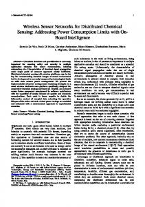
for a certain amount of time ( ) to hear from any potential children. If any child responds within this period, the previous procedure of assigning one byte ID repeats itself. If no child responds, the node considers itself a leaf node. All messages except the ones of type 1 are exchanged in a reliable way. A message of type 2, which contains the random 4-byte integer chosen by a child node, is confirmed by the reception of a message of type 3 (reinitialization message) or type 4 (containing a 1-byte assigned ID). A message of type 3 is resent if the parent node receives a second message of type 2 with the same 4-byte ID. A message of type 4 is confirmed through the reception of the confirmation message of type 5. If a message is not confirmed within a random period chosen uniformly between and , the message is resent. The node keeps checking for a confirmation and resending until the message is confirmed. Figure 1 illustrates the messages exchanged between a parent node and a child node during phase 1 when no reinitialization message is sent. A reinitialization message makes the child node resends the message of type 2. At the end of this exchange, the child node has a temporary ID that is 1 byte longer than the one of its parent node. The child node then sends its own message of type 1. Algorithm III-A gives the pseudo code of the first phase. Note that at the end of this PSfrag replacements phase every node knows the temporary ID of its parent node. The parent ID is equal to the node ID without the last byte.
Algorithm 1 Phase 1: Temporary ID Assignment if
is true then
send an initialization message of type 1 end if if receive message of type 2 then if a child already have same intId then send reinitialization message of type 3 end if then if no child already has same add to children list choose a random time rt schedule checking for confi rmation at rt send message of type 4 with ChildIdB end if end if if receive msg message of type 5 then then if fi nd , the corresponding child end if end if if receive fi rst message
of type 1 then
choose a random 4-byte choose a random time schedule checking for confi rmation at send message of type 2 with end if message of type 3 then if receive choose a different random 4-byte choose a random time schedule checking for confi rmation at send message of type 2 with end if TempID: 163.25 TempID: 163.25.41 message of type 4 then if receive if is true then update type 5, t3 resend message of type 5 end if Parent node type 4, t2 Child node if is not true then type 2, t1 and update update type 1, t0 choose a random time schedule sending message of type 1 at send message of type 5 PSfrag replacements Fig. 1. One step of phase 1 with no reinitialization message end if end if
B. Phase 2: Collecting the Sub-Tree Sizes TempID: 41 Size: 403
t4 p ty
e
6,
typ
type 6, t2
t5
e7
, t1
6,
7,
e
e
ty p
p ty
TempID: 41.62.1 Size: 300
TempID: 41.62 Size: 402 type 7, t3
t0
type 6, t6
type 7, t7
In this phase, nodes report their sub-tree sizes from the leaf nodes to the root node. The sub-tree size of a particular node is the number of nodes contained in the tree rooted at that node at the end of phase 1. A node that is declared leaf at the end of phase 1 considers its sub-tree size to be 1 and sends it as a message of type 6 to its parent. A non-leaf node waits until it receives sub-tree sizes from all of its children nodes before sending its sub-tree size to its parent. Sub-tree size messages are confirmed by the parent node with a confirmation message of type 7. Figure 2 illustrates the message exchange during phase 2 to collect the sub-tree sizes. When the initiator receives sub-tree size messages from all of its children, it knows the total number of nodes in the network. This total is used to compute the minimum number of bytes needed to code a unique final ID for each node in the network. These IDs are assigned in phase 3 of the algorithm. Algorithm III-B gives the pseudo code of the second phase.
TempID: 41.62.2 Size: 1 TempID: 41.62.0 Size: 100
Fig. 2.
One step of phase 2
PSfrag replacements
Note that at the end of this phase every node knows its subtree size as well as the sub-tree size of each of its children nodes.
FinalID: 98
type 8, t0
Algorithm 2 Phase 2: Sub-tree Sizes Collecting
is transmitting a Assuming a single channel, if a node message to a node , a collision occurs if is already in the process of receiving from a different node. The algorithm does not assume the existence of any specific MAC address. In particular, no collision avoidance mechanism is required.
t7 p ty
e
9,
type 9, t3
t5 9, e ty p
D. Collision Handling
t6
In this phase, the final unique IDs are assigned by each parent node to its children nodes starting from the root. Final IDs are coded using the same number of bytes (i.e., 1, 2, 3, or 4) for all nodes. The initiator is assigned an ID of 0. It sends a final ID message (message of type 8) to each of its children nodes. Each message contains a unique ID and the number of bytes to be used to code IDs. Final ID messages are confirmed with messages of type 9. Each node receiving a message of type 8 takes the ID it contains as its final ID and knows that a number of IDs starting from its ID and containing as many IDs as needed is reserved for the IDs of the nodes in its sub-tree. Each non-leaf node receiving a final ID message confirms it and assigns IDs to its children nodes in a similar way. Figure 3 illustrates the message exchange during phase 3 to allocate the final IDs. Each node allocates its ID plus to the child 1 to its first child and then allocates with , where is the sub-tree size of the child. Algorithm III-C gives the pseudo code of the third phase. At the end of this phase, every node in the network knows its final ID. These final IDs are coded using the minimum number of bytes.
8,
Fig. 3.
C. Phase 3: Final Unique ID Assignment
e
FinalID: Size: 100100
Size: 403
is not true then
p ty
t4 FinalID: 200 Size: 300
type 8, t2
e 8,
send message of type 7 choose a random time schedule checking if all sub-tree sizes received at end if end if if leaf is true then choose a random time schedule checking for confi rmation at send message of type 6 end if message of type 7 then if receive if is not true then update end if end if if sub-tree size messages received from all children and choose a random time schedule checking for confi rmation at send message of type 6 end if
FinalID: 99 Size: 402
ty p
if receive message of type 6 then fi nd , the corresponding child if is true then resend message of type 7 end if is not true then if and
type 9, t1
SubT5
FinalID: 500 Size: 1
One step of phase 3
Collision is handled in the sense that all messages except the initialization message (message of type 1) received by a node are confirmed by an acknowledgment message. Before sending a message, a node chooses randomly an integer number between 0 and , and waits for a time equal to . If it does not receive the confirmation within the random waiting time, it resends the message and keeps doing so until receiving the confirmation. The node adapts the parameter to the traffic condition. In fact, this parameter is increased by half of its initial value ( ) every time an expected confirmation is not received, unless has already reached an upper . Upon the reception of a message, limit set to is reduced by half of , unless a lower bound, set to the initial value, is already reached. For the message of type 1, it is assumed that every node has several neighbors. Each neighbor sends an initialization message at different times (randomly chosen after the first phase). Therefore, a node has several possibilities of receiving an initialization message. IV. T HEORETICAL A NALYSIS This section contains the theoretical evaluation of the unique ID assignment algorithm. In particular, the correctness of the algorithm is analyzed. We also prove that the algorithm terminates naturally and give an upper limit on the average energy consumption per node. Since the initial assignment messages (of type 1) are sent in a reliably, we also analyze the probability of a node being left out by the algorithm. Such a node does not participate in the algorithm and is not assigned an ID. A. Model The evolution of each node, except for the initiator, is modeled as a stochastic process with state space of . The different states are defined as follows:
Algorithm 3 Phase 3: Final IDs Assignment if sub-tree size messages received from all children and compute , the number of bytes
choose random time schedule checking for confi rmation at send message of type 8 to fi rst child with end if if receive message of type 9 then , the corresponding child fi nd if is true then ignore end if is not true then if if more nodes in the children list then choose random time schedule checking for confi rmation at send message of type 8 to next child with end if end if end if if receive message of type 8 then is true then if resend fi nal ID confi rmation message of type 9 end if is not true then if
on its current state as well as the states of the neighboring nodes. In fact, the neighbors influence the node state in several ways. A non-initiator node currently in state 0 can go to state 1 only if at least one of its neighbors is already in state 2. A non-leaf node in state 3 can change to state 4 only if all of its children nodes (a sub-set of its neighbors) are already in state 4. A non-initiator node currently in state 4 can go to state 5 only if its parent node is already in state 5. More generally the neighbors affect the probability of change in the sense that they can cause collisions if transmitting simultaneously. Collisions cause messages to be retransmitted and delay state changes. We define the probability ( ) as the probability that when PSfrag replacements the node is in state at time , it goes to state in the next step ( ) with between 0 and 4. As stated earlier, the value of ( ) depends on the current state of the node as well as the current states of its neighbors, in particular its parent and children nodes. Figure 4 gives the state diagram. is true then
State 1: Initialized send message of type 9 to parent node choose random time schedule checking for confi rmation at send message of type 8 to fi rst child with end if end if
1) State 0: A node is in state 0 if it did not yet receive any initialization message (message of type 1) 2) State 1: A node is in state 1 if it has already received an initialization message, is still waiting for its temporary ID to be confirmed by its parent node 3) State 2: A node is in state 2 if its temporary ID has been confirmed by its parent node, but it did not yet send a message of type 1 4) State 3: A node is in state 3 if its temporary ID has been confirmed by its parent node, it has sent a message of type 1, but did not yet send its sub-tree size message. This could be because it is still waiting to know if it is a leaf, or is still waiting for at least one child node to report the size of its sub-tree. It could also be during the period after receiving all sub-tree sizes, but the scheduled time to send its sub-tree message has not been reached 5) State 4: A node is in state 4 if it has already reported its sub-tree size to its parent node but is still waiting to receive its final ID 6) State 5: A node is in state 5 if it has already received its final ID Clearly, state 5 is a stable state after which the node does not go back to any other state. It is also clear that a node can only go to the next higher state or remain in its current state. That is, for example, a node in state 3 can only go to state 4 or remain in state 3. The probability that a node changes its state depends
State 2: Temp ID
State 0: Inactive
State 3: Init Sent
State 5: Final ID
State 4: Size Recd
Fig. 4.
States diagram
B. Performance of the Algorithm In this subsection, several properties of the algorithm are given. In particular, the correctness and termination of algorithm are studied. We also study the probability of a node not being assigned an ID at the end of the algorithm. This is a measure of the effectiveness of the algorithm. Due to the page limit, the proofs of different lemmas in this subsection can be found in [13]. Before studying the correctness of the algorithm, we look at the possibility of two nodes with the same parent receiving the same temporary ID. This occurs only when two children of the same node choose the same 4-byte ID in first phase and respond simultaneously with messages of type 2 to the initialization message and their parent receives only one of the two messages. For the two nodes to end up with the same temporary ID, they need also to send simultaneously the confirmation message of type 5 and for their parent to receive one and only one of these messages. as the probability of two nodes having two We define identical temporary IDs. As we can see, is very low because the occurrence of two nodes having two identical
temporary IDs is conditioned to the occurrence of a successive number of independent events each having a very low probability. In fact, , where is the probability of any two nodes in the network with the same parent choosing the same 4-byte integer. It can be proved that for a network of nodes each having no more than 256 neighbors, we have . For , we obtain . The following lemma states the correctness of the algorithm. This lemma is proved in [13]. Lemma 1: If the algorithm terminates, each participating node has a unique ID with a high probability of , where is as defined above. The following lemma, proved in [13], shows that if nodes do not die during the execution of the algorithm, then the algorithm terminates. Lemma 2: If all nodes that received an initialization message remain alive, then the algorithm will terminate. We now determine the probability that a message is successfully transmitted by the second trial. A message is not successfully transmitted if a collision occurs. A collision , when it does not reis detected by the sender node, ceive the corresponding confirmation message in a randomly predetermined time period. As explained in Subsection IIID, the length of this time period is uniformly distributed between and . If no confirmation is received, the message is resent at the end of this period. A collision occurs if the receiving node, , is currently in the process of receiving a different message. It also occurs if a different neighbor of broadcasts a message while the current message is being received. If the size of the current message is S bytes and the capacity of the radio is B kbps, the transmission (reception) time of the message is given by: . Suppose that the transmission starts at the current message is not received (collision) if at least one of the other neighbors transmits a message in the time interval . If has k neighbors, including the sender , each neighbor transmits at most one message during each period of length , where is the initial value of . Consequently, there are at most messages sent by the other neighbors. Each message is followed by a confirmation message except for a message of type 1 or when confirming a previous message from . Therefore, there are at most confirmation messages and a total of messages. Assuming that all messages have approximately the same size S, the current message encounters a collision if its reception starts in one of at most transmission periods of length . The following lemma, proved in [13], bounds the probability that a message is received by the second trial. is such that Lemma 3: If , then the probability of a message successfully received upon second transmission is at least . , we can This demonstrates that by appropriately setting guarantee a high probability of transmission of messages by the second trial. For a numerical example, we assume that the
radio transmission rate is , which is reasonable for current technology: transmission rate for MICAz motes for example is 250 kbps. We also assume that , the network having a density of 21. The message size is function of the number of hops from the base station since each address is composed of one byte per hop. Let assume that at most . This limit holds even for large networks with low densities. Then we have: . Clearly, we can see that by setting initially to , we obtain the following high probability of successful transmission by the second trial: . By following the same reasoning as above, we can bound the probability of a node not assigned an ID at the end of the algorithm. This occurs if the messages of type 1 (initialization messages) from all of its neighbors are lost. Since each of these messages is sent at a random time, we obtain the following lemma, proved in [13]. Lemma 4: If k neighbors of a node are assigned IDs, then the probability of the node being left out is at most . Again, this probability can be controlled through the parameter . A performance measure of the algorithm is the amount of energy consumed per node during the execution of the algorithm. Since the processing energy is negligible compared to the communication energy, we are taking into account only the latter. The following lemma, proved in [13], bounds the average communication energy consumption per node. Lemma 5: If on average each node has neighbors and the average message size in the network is bits, then the average communication energy consumption is bounded by , where and are respectively energy consumption per bit for transmission and reception, with probability , where is as defined in lemma 3. V. S IMULATION R ESULTS In this section, we show the performance of the algorithm under different simulation settings. We study the effect of different parameters on the performance. In particular, we study the effect of the network size, network density, and initial on the execution time, the percentage of value of nodes assigned an ID at the end of the algorithm, and the probability of a message being retransmitted. Simulations are performed using GTSNetS (the Georgia Tech Sensor Network Simulator) [14], [15]. Nodes are distributed in an equi-distant fashion in a square region with the initiator located at the center of the region. The distance between two successive nodes is fixed at 20 meters. The network density is changed by modifying the transmission range: transmission range of 21 meters for a density of 4, 30 meters for a density of 8 and so on. Messages exchange is performed entirely using broadcasts. Channel sensing is performed before sending a message, which reduces the collision probability. Under each setting, each simulation was run 10 times. An average for these 10 runs is used as the final result.
Figure 5 plots the execution time of the algorithm as a function of the network size while maintaining a fixed network density of 4 neighbors. As expected, the execution time increases with the network size, but remains relatively short (less than 30 minutes for a network of 10,000 nodes). Execution time Vs. network size 30
TimeWaitI = 1.5 TimeWaitI = 2 TimeWaitI = 2.5
Execution time (minutes)
25
20
15
10
5 1000
2000
3000
4000
5000 6000 Network size
7000
8000
9000
can also see that for a specific network size, we can obtain a very high percentage of ID assignments by increasing the initial value of to a high enough value. However, as this value increases the execution time also increases. With a initially of 2.5 seconds, we can obtain a percentage of about 99.5% even for a large network of 10,000 nodes. Figure 8 plots the percentage of nodes assigned a unique ID at the end of the algorithm as a function of the network density for a network of 1,000 nodes. We can see that the percentage of nodes with an assigned ID at the end of the algorithm decreases as the density increases. This is due to the fact that higher density increases the probability of collisions, which reduces the probability of successful reception of messages of type 1 even though more messages are sent in each neighborhood. Messages of type 1 are not retransmitted, and their loss reduces the probability of a node participating in the algorithm.
10000
Assignment Runtime probability Vs. network Vs. network size size 100
Fig. 5.
TimeWaitI = 1.5 TimeWaitI = 2 TimeWaitI = 2.5
Execution time Vs. network size
Assignment probability (%)
99.8
Figure 6 plots the execution time of the algorithm as a function of the network density for a network of 1,000 nodes. We can see that the execution time decreases as the density increases. This is due to the fact that density is increased by increasing the communication range, which reduces the number of hops between the initiator and the leaf nodes. The execution time remains relatively short even for a network of low density.
99.6
99.4
99.2
99
98.8
98.6 1000
2000
3000
4000
Execution time Vs. network density 10
TimeWaitI = 1.5 TimeWaitI = 2 TimeWaitI = 2.5
Fig. 7.
9
5000 6000 Network size
7000
8000
9000
10000
Assignment probability Vs. network size
Execution time (minutes)
8
Collision probability Vs. network density
7 100 6
98
4
2
4
Fig. 6.
6
8
10 12 Network density
14
16
18
20
Execution time Vs. network density
Assignment probability (%)
5
3
TimeWaitI = 1.5 TimeWaitI = 2 TimeWaitI = 2.5
99
97 96 95 94 93 92
Both Figure 5 and Figure 6 show that the execution time . This is not increases with the initial value of surprising since nodes wait longer before resending lost messages and before forwarding the initialization messages. This makes the overall algorithm take more time to terminate. It is, therefore, desirable to keep the initial value of as low as possible. Figure 7 plots the percentage of nodes assigned a unique ID at the end of the algorithm as a function of the network size with a network density of 4 neighbors. We can see that this probability decreases as the size of the network increases. We
91 2
Fig. 8.
4
6
8
10 12 Network density
14
16
18
20
Assignment probability Vs. network density
Both Figure 7 and Figure 8 indicate that we can increase the probability of nodes participation in the algorithm by increasing the initial value of . However, such an increase causes the execution time to increase which is not desirable. Thus, there is a tradeoff between the percentage of assigned IDs and the execution time.
Finally, we study the probability of collisions under various simulation settings. Figure 9 plots the probability of a message being retransmitted because of collision as a function of the network size. We can see that this probability increases with size. This is due to the fact that messages are longer on average since more nodes are located many hops away from the initiator. Longer messages take more time to transmit, which makes the occurrence of a collision more likely. As expected, the probability of collision diminishes, when the value of increases. Assignment Collision probability probabilityVs. Vs.network networksize size 9.2
TimeWaitI = 1.5 TimeWaitI = 2 TimeWaitI = 2.5
9
ACKNOWLEDGMENT This work is supported in part by NSF under contract numbers ANI-9977544, ANI-0136969, ANI-0240477, ECS0225417, CNS 0209179, and DARPA under contract number N66002-00-1-8934.
Collision probability (%)
8.8
8.6
8.4
8.2
R EFERENCES
8
7.8
7.6 1000
2000
Fig. 9.
3000
4000
5000 6000 Network size
7000
8000
9000
10000
Collision probability Vs. network size
Figure 10 gives the collision probability as a function of network density for a network of 1,000 nodes. We can see that collision is more likely in a network with higher density. This is not surprising since more nodes are competing for each channel. We can also see that the collision probability can be controlled by increasing the value of . Collision probability Vs. network density 15
TimeWaitI = 1.5 TimeWaitI = 2 TimeWaitI = 2.5
14
Collision probability (%)
13
12
11
10
9
8
7 2
Fig. 10.
VI. C ONCLUSION We presented a solution to the global ID assignment problem in sensor networks. Our solution aims at assigning unique IDs to each node using the minimum number of bytes required to code these IDs. This was obtained using a 3-phase approach. In the first phase, temporary long IDs are assigned. These temporary IDs are used in the second phase to reliably determine the exact size of the network and, therefore, the minimum number of bytes to use. In the third phase, final IDs coded using the minimum number of bytes are assigned. We demonstrated that the proposed algorithm can be tailored to obtain excellent results, both in terms of the percentage of participating nodes and the execution time.
4
6
8
10 12 Network density
14
16
18
20
Collision probability Vs. network density
Based on the results, we can state that the initial value of plays a central role in the algorithm. It needs to be set appropriately so as to maximize the probability of nodes being assigned an ID at the and of the algorithm and minimize the collision probability while keeping the execution time under control.
[1] D. E. Chalermek Intanagonwiwat, Ramesh Govindan, “Directed diffusion: a scalable and robust communication paradigm for sensor networks,” in Proceedings of the 6th annual international conference on Mobile computing and networking, pp. 56–67, August 2000. [2] Y. Yu, R. Govindan, and D. Estrin, “Geographical and energy aware routing: A recursive data dissemination protocol for wireless sensor networks,” Tech. Rep. TR-01-0023, UCLA/CSD, 2001. [3] A. Dunkels, J. Alonso, and T. Voight, “Making tcp/ip viable for wireless sensor networks,” in First European Workshop on Wireless Sensor Networks (EWSN), 2004. [4] C. Karlof and D. Wagner, “Secure routing in wireless sensor networks: Attacks and countermeasures,” in Proceedings of the 1st IEEE International Workshop on Sensor Network Protocols and Applications, 2003. [5] W. Ye, J. Heidemann, and D. Estrin, “An energy-effi cient mac protocol for wireless sensor networks,” in Proceedings of INFOCOM, 2002. [6] A. S. Tanenbaum, Computer Networks. Englewood Cliffs, 1989. [7] J. R. Smith, “Distributing identity,” IEEE Robotics and Automation Magazine, Vol.6, No.1, March 1999. [8] C. Schurgers, G. Kulkarni, and M. B. Srivastava, “Distributed ondemand address assignment in wireless sensor networks,” IEEE Transactions on Parallel and Distributed Systems, Vol.13, No.10, pp. 1056-1065, October 2002. [9] D. Estrin, J. Heidemann, and S. Kumar, “Next century challenges: Scalable coordination in sensor networks,” in Proceedings of MOBICOM, pp. 263–270, 1999. [10] M. Ali and Z. A. Uzmi, “An energy effi cient node address naming scheme for wireless sensor networks,” in Proceedings of the International Networking and Communications Conference (INCC), 2004. [11] W. B. Heinzelman, A. P. Chandrakasan, and H. Balakrishnan, “An application-specifi c protocol architecture for wireless microsensor networks,” IEEE Transactions on Wireless Communications, Vol.1, No.4, October 2002. [12] W. B. Heinzelman, J. W. Kulik, and H. Balakrishnan, “Adaptive protocols for information dissemination in wireless sensor networks,” in Proceedings of MOBICOM, 1999. [13] E. Ould-Ahmed-Vall, D. M. Blough, B. S. Heck, and G. F. Riley, “Distributed global identifi cation for sensor networks,” Tech. Rep. GITCERCS-05-17, Georgia Tech/CERCS, 2005. [14] E. Ould-Ahmed-Vall, G. F. Riley, and B. S. Heck, “Simulation of largescale sensor networks using gtsnets,” in to appear in Proceedings of Eleventh International Symposium on Modeling, Analysis and Simulation of Computer and Telecommunication Systems (MASCOTS’05), 2005. [15] E. Ould-Ahmed-Vall, G. F. Riley, and B. S. Heck, “Gtsnets: the georgia tech sensor network simulator,” in Poster Papers Proceedings of the 7th ACM International Symposium on Modeling, Analysis and Simulation of Wireless and Mobile Systems (MSWiM), 2004.