Error Distribution for Gene Expression Data

Error Distribution for Gene Expression Data Elizabeth Purdom Department of Statistics, Sequoia Hall, CA 94305 Stanford University

Susan Holmes Department of Statistics, Sequoia Hall, CA 94305 Stanford University

May 12, 2005

1

Introduction

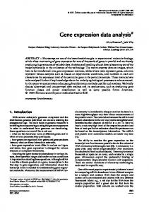
Microarrays allow the researcher to investigate the behavior of thousands of genes simultaneously under various conditions. The insights possible from such experiments are vast, but the number of errors due to the complexity of the experiments is also substantial. A great deal of statistical research has focused on eliminating known biases introduced at different stages of the process and then discriminating which genes are differentially expressed across the conditions of interest (for example observations from cancer patients versus healthy patients). We propose the use of a known parametric model as an approximation of the distribution of the log-ratios of measured gene expression across genes – the Asymmetric Laplace Distribution (Kotz et al., 2001). Namely, if all the genes on one array are considered as separate independent observations, the distribution of the log-ratio of the expression values is well approximated by the Asymmetric Laplace Distribution. Figure 1 gives an example of the fit of the Asymmetric Laplace Distribution as compared to the Normal distribution. The Asymmetric Laplace captures the peak at the center of the data as well as the asymmetry in the distribution. Genes expression ratios, of course, are not independent. However there are many instances, particularly in normalization of the arrays, where the statistical analysis does assume independence among the genes. In the two-color microarray datasets for which we fit the Asymmetric Laplace distribution (described in Section 4.1), the model usually gave a reasonable fit to the gene expression data and greatly improved upon the Normal distribution. As an approximating distribution, this distribution provides an alternative parametric model from the normal distribution to explore the effects of statistical procedures. The Laplace distribution has a appealing representation of a mixture of normals with differing variances. Furthermore, the Laplace distribution gives a conceptually simple adjustment to existing normalization methods which gives robust as well as parametrically justified procedures.

1

Asym. Laplace Normal

−1.0

−0.5

0.0

0.5

1.0

Figure 1: Histogram of gene expression of all genes on a single cDNA microarray from T-Cell Data (described below in Section 4.1). Corresponding Asymmetric Laplace and Normal distribution overlayed, with parameters estimated using maximum likelihood estimates.

2

Brief Background

A two-color microarray experiment takes two different samples of cDNA tagged with different dyes, red (Cy5) and green (Cy3). The two samples are hybridized to known DNA sequences that are spotted on a glass slide. After hybridization, the slide or array is scanned to measure the dye intensities. Higher dye intensities imply greater presence of the mRNA in the sample corresponding to that dye. Typically, one of the samples is a standard reference made of mRNA from pooled cell lines and the other sample is from the observation. A microarray experiment will repeat this for each observation. Each array will give information on the relative gene expression of the observation compared with the standard reference; these relative gene expression patterns can be compared among patients. When done for classification of conditions, the experiment is designed so that the observations come from different known conditions, and the relative expression can be compared between these groups. Differentially expressed genes are genes that are expressed differently (relative to the reference) between the conditions of interest. However technical aspects of the experiment, such as the position of the spot on the chip or different levels of the incorporation of the Cy5 and Cy3 dyes, mean that the measured expression levels have built in biases due to the technicalities of the experiment. Indeed, even for “self-self” hybridization experiments where both samples on the array come from the same original sample, the error in measurement 2

of relative gene expression is biased. Normalization methods try to correct the expression levels within an array to counteract this bias. Generally such methods assume that for each array, only a small proportion of the total genes should be expressed differently from the reference sample. Thus, we expect the difference in gene expression between the red and the green channel to be due to just random fluctuation. In other words, the resulting gene expression represents observations from some error distribution. Normalization techniques transform the data so that the distribution of gene expression across the array reflects this assumption. One common technique in cDNA arrays is to look at the plot of the difference of the red and green against the average expression (on a log scale) and then transform the data so that the log difference is centered at zero, using for instance LOWESS regression (Dudoit and Yang, 2003). These can be done globally for all of the genes at once, or separately based on the layout information of the genes on the slide. Another approach, variance stabilizing normalization (VSN), further transforms the data to stabilize the variance across expression level (see Durbin et al., 2002; Huber et al., 2003). The distribution of the normalized gene expressions, while similar across arrays, is often far from normal, regardless of the normalization methods. Rather, the distribution tends toward heavy tails and asymmetry of varying degrees (see, for example, Figure 2). Traditional centering and scaling with the mean and the standard deviation suggested by a normal distribution approximations are sensitive to outlying points. Because of the heavy tails and non-normality of the data, many authors suggest recentering and rescaling microarray data with more robust estimates of location and variance, such the median and mean/median absolute deviation, respectively (Yang et al., 2001). This suggests an error distribution that estimates the location parameter with the median and the scale parameter with the mean absolute deviation (MeanAD1 ). Such a distribution exists and is called Laplace’s First Error Distribution, a Laplace distribution, or a double exponential distribution. The classical Laplace distribution is symmetric around its location parameter; however, gene expression data often displays signs of asymmetry. A known generalization of the Laplace distribution, the Asymmetric Laplace, allows for asymmetry if necessary (see Figure 5).

3

Overview of the Laplace Distribution

The Laplace distribution (L(θ, σ)) has two parameters, a location parameter θ and a scale parameter σ. The density function is √ 1 fY (y) = √ exp(− 2|y − θ|/σ), 2σ

σ>0

1 MAD often refers to the median absolute deviation, rather than the mean absolute deviation, thus we use the abbreviation MeanAD

3

−1.0

−0.5

0.0

0.5

1.0

−1.5

−1.0

−0.5

(a) T-Cell

−1.0

−0.5

0.0

0.5

0.0

0.5

1.0

(b) Self-Self

1.0

1.5

2.0

(c) Swirl Zebrafish

−1.0

−0.5

0.0

0.5

(d) Yeast

Figure 2: Histogram of gene expression of all genes on a single array from different Microarray datasets (after normalizations as described below in section 4.1).

4

1.0

1.5

L(0,1) N(0,1)

−4

−2

0

2

4

Figure 3: Density Plot of standard L(0, 1) and a standard normal N (0, 1) See Figure √ 3 for a plot of the density. The maximum likelihood estimates of θ and s = σ/ 2 are the median and the MeanAD respectively. A L(θ, σ) distribution has expected value θ and variance σ 2 = 2s2 . The L(θ, σ) distribution has “heavier tails” than the normal, meaning that there is more probability of extreme values than under a normal distribution. In addition, the L(θ, σ) distribution concentrates more probability in the center than a normal distribution. Distributions have been proposed in other contexts that adjust the Laplace distribution so as to admit a skewness parameter in the distribution. In particular, a family of distributions proposed by Hinkley and Revankar (1977), the Asymmetric Laplace Distribution (AL(θ, µ, σ)), introduces a skew parameter, µ (or κ in a different parameterization), to the classical Laplace distribution, while maintaining basic properties of the Laplace distribution. The density of the AL(θ, µ, σ) can be explicitly written (see Figure 4 for illustrations of the distribution): ( √ √ 2 κ exp( − σ2κ |x − θ|) if x≥θ √ f (y) = (1) 2 − 2 σ 1+κ exp( σκ |x − θ|) if x 0. As would be expected, the traditional, symmetric Laplace distribution with no skew is a special case of µ = 0 (or κ = 1). θ and σ remain location and scale parameters, so that if Y ∼ AL(θ, µ, σ) then Y σ−θ ∼ AL(0, µ/σ, 1) The distribution can also be parameterized in terms of κ, as in Equation (1). If Y ∼ AL(θ, κ, σ) then Y σ−θ ∼ AL(0, κ, 1), so κ does not change with shifts or (positive) scalings of

5

µ=0 µ = 0.5 µ=1 µ = 1.5 µ=2

−4

−2

0

2

4

Figure 4: Density Plot of Asymmetric Laplace AL(θ, µ, σ), with θ = 0 and σ = 1, for varying values of µ the random variable Y . The expectation and variance of an AL(θ, µ, σ) are E(Y ) = θ + µ var(Y ) = σ 2 + µ2

Note the variance is not independent of the mean unless µ = 0 – the case of the symmetric Laplace Distribution. The maximum likelihood estimates of θ, σ and µ can be determined and are given in Kotz et al. (2001, p.173-174).2 The median is the θ that minimizes 1X 1X 1X |Xi − θ| = (Xi − θ)+ + (Xi − θ)− n n n = α(θ) + β(θ) where α(θ) = β(θ) =

1X (Xi − θ)+ n 1X (Xi − θ)− n

2

Note that the MLE given here is different than the p result given in Kotz pP et al. (2001, P + + p. 173) There the authors minimize h(θ) = 2log( (X (Xi − θ)− ) + i − θ) pP P + − (Xi − θ) (Xi − θ) (3.5.118). However there seems to be an error in equation (3.5.110) from which h(θ) is derived, and the second term in h(θ) should not be included.

6

α(θ) is the sum of how much larger the data points are than θ while β(θ) is the sum of how much smaller the data points are than θ. Then the MLE θˆ for θ in the asymmetric distribution minimizes p 1X |Xi − θ| + 2 α(θ)β(θ) (2) n The difference is the second term involving α(θ) and β(θ) again, which pushes the estimate of θ toward the mode of the distribution. If the distribution is symmetric then these will be the same, and the MLE will still be the median. But in the non-symmetric case, the MLE of θ, the location parameter, is no longer exactly the median, but is a different order statistic that depends on the skewness of the data. Once θˆ is found, the MLEs for µ and σ are: ¯ − θˆ µ ˆ = X q  q √ q 4 ˆ ˆ ˆ ˆ σ ˆ = 2 α(θ)β(θ) α(θ) + β(θ)

When the data is roughly symmetric σ ˆ will be close to the MeanAD and θˆ will be close to the median. The maximum likelihood estimates are asymptotically normal and efficient (Kotz et al., 2001) with asymptotic covariance matrix: 

√

2 2 4 σ(1 +κ ) 2 1+κ2 2

σ2 √

1  2 σ(1 + κ2 )  4 n √ 2 2 1 4 σ ( κ − κ)

σ 1 4 (κ

ψ(t) =

− κ)(1 + κ2 )

√



2 2 1 4 σ ( κ − κ)  σ 1 2 ) ( − κ)(1 + κ  4 κ    σ(κ+ 1 ) 2

1 1 2 2 1 + 2 σ t − iµt

(3)

κ

2

!τ (4)

The AL(θ, µ, σ) distribution has τ = 1, and generally the sum of n identically and independently distributed (i.i.d) AL(θ, µ, σ) random variables is distributed as a generalized Laplace distribution with τ = n. This means that the sum of Generalized Asymmetric Laplace random variables is still distributed as Generalized Asymmetric Laplace but with a different τ parameter.

4 4.1

Applications to Microarray Data Fitting AL(θ, µ, σ) to Two-Color Microarray Data

We examined several microarrays from published microarray experiments. The first dataset was a set of 70 arrays from sorted T-cells compared to classical human reference cell-lines by competitive hybridization on Agilent cDNA chips (Xu et al., 7

2004). The data was normalized as described in Xu et al. (2004) using the vsn package in R (Huber and Heydebreck, 2003), which applies a generalized-log transformation to stabilize the variance across expression values. The difference of the two channels gave the gene measurement. The second dataset (B) consists of self-self hybridizations of 19 different cell lines, as well as the Stratagene universal reference RNA (Yang et al., 2002). The self-self arrays were normalized using loess smoothing, as described in the paper, though we applied the loess smoothing separately per print-tip group. Log-differences of the two channels were then used for the measurement per gene. Dataset (C) is two sets of dye-swap experiments comparing a swirl mutant zebrafish with wildtype. It is available as a dataset with the R package marrayClasses (Dudoit and Yang, 2002; Wuennenberg-Stapleton and Ngai, 2001). The zebrafish arrays were also normalized using print-tip group loess smoothing and then log-differences were used as gene measurement, as described in the marrayNorm package. The last dataset (D) is of 86 haploid segregants from a cross between laboratory and wild strain yeast (Saccharomyces cerevisiae) from Yvert et al. (2003). The progeny was measured with two arrays each, with dyes swapped, and the parent strains measured with four arrays each, also with the dyes swapped. The reference sample for all arrays was an independent sample of the laboratory strain. This data is available on NCBI’s Gene Expression Omnibus (GEO) database. Yvert et al. (2003) normalized the data by subtracting off the mean of the log-ratio. In what follows, we normalized the data using the vsn package in R. In the following exposition, we show results from a single array from each of these datasets (see Supplementary Figures for all of the arrays).3 We also examined another cDNA dataset, included in the supplementary figures, of tumor samples from diffuse large B-cell lymphoma patients (Alizadeh et al., 2002). This data was normalized using the vsn package as well. We estimated maximum likelihood estimates and asymptotic standard errors of the parameters of a AL(θ, µ, σ) distribution for all of the arrays (see Table 1 and Supplementary Figures 13). Notice, that while the parameter µ depends on the scale of measurement, the parameter κ is a comparable measure of skewness across the datasets regardless of the scale. We see in the cDNA arrays that κ is close to one across the arrays, indicating small levels of skewness, and often not significantly different from one. In Figure 5 we overlay the estimated AL(θ, µ, σ) density on the observed histograms, where θ, σ and µ are estimated with their respective maximum likelihood estimates. For comparison, we also overlayed the estimated normal density. From these density plots we can see that the AL(θ, µ, σ) distribution is capturing something of the “spirit” of the density, with peaked concentration in the center and 3 From the T-Cell dataset, we used array 15, the naive t-cells of a healthy patient. With the self-self hybridizations, we used array 5, the KM12L4A cell line RNA as shown in Figure 2 in Yang et al. (2002). From the Zebrafish dataset, we used array 3, “swirl.3.spot”, where Cy3 was the mutant and Cy5 the wildtype. For the yeast data, we used 5-3-dCy5, where the reference sample was in Cy3 (array 45).

8

θˆ T-Cell Self-Self Zebrafish Yeast

0.039 −0.001 −0.104 −0.002

(0.003) (0.002) (0.005) (0.004)

κ ˆ 1.174 1.002 0.792 0.930

(0.011) (0.007) (0.002) (0.013)

0.304 0.243 0.430 0.283

σ ˆ

µ ˆ

Median

MeanAD

(0.005) (0.009) (0.005) (0.004)

−0.069 −0.001 0.143 0.029

0.006 −0.001 −0.008 − 0.002

0.221 0.172 0.318 0.193

Table 1: Maximum Likelihood Estimates of the parameters for microarray data, with standard error estimates for θ, κ, σ in parenthesis.

heavy tails. Using Quantile-Quantile Plots (Q-Q Plots), which better emphasizes the fit of the distribution in the tails, we see in Figure 5 that the Q-Q plots are linear. Only a few points out of the thousands of observations deviate significantly from a straight line. This indicates a reasonable fit to the Asymmetric Laplace distribution and is much preferred to the Normal distribution (also in Figure 5). For the arrays not shown, the fit is often comparable to those shown here, though some have greater deviations in the tails and others would have to be classified as a misfits. In general, the Asymmetric Laplace performs better than the corresponding normal (see Supplementary Figures 9, 10, 11, 12)4 . In particular, the tails of the distribution, as best demonstrated in Q-Q Plots, are in good agreement with the Asymmetric Laplace, even in those cases where the center of the distribution seems better described by a Normal distribution. Since graphical methods lack rigor, we would like to perform tests to determine how well the AL(θ, µ, σ) distribution fits this data. We examined two standard tests: the Kolmogorov-Smirnov (K-S) test and the Anderson-Darling (A-D) test. The Kolmogorov-Smirnov test takes as the test-statistic the maximum absolute distance between the empirical and the theoretical CDF, while the Anderson-Darling test uses a weighted integral of the squared distance between the empirical and theoretical.5 Almost all of the arrays result in an extremely significant difference from the AL(θ, µ, σ) at standard testing levels of testing (e.g. α = .05, .01). The reason for this, however, probably comes from the enormous sample size involved (n ≈ 10, 000) so that the test is highly sensitive to any deviations from the null. This is a well-known statistical paradox: with large amounts of real data, every hypothesis test will reject point nulls (see, for example Efron and Gous, 2001; Lindsey, 1999). In general the statistics are less extreme using the Laplace as a null distribu4 In the T-cell data the data is in 5 batches, and batch two seems to have severe problems with the AL(θ, µ, σ) fit. 5 Since we must estimate the unknown parameters of the AL(θ, µ, σ) distribution, asymptotic estimates of the distribution of the test-statistics do not exist. One can use the half-sample method (Stephens, 1986), where the unknown components are estimated with half of the data and then the test is run, using these estimates, on the entire dataset. Given the size of the sample, the MLE estimates are stable, so the effect of the half-sample method is negligible.

9

(a) T-Cell (one point excluded on each tail)

(b) Self-Self

Figure 5: Histograms from Figure 2 overlayed with estimated Asymmetric Laplace distribution and Normal Distribution. Parameters of both distributions estimated with maximum likelihood estimates. Q-Q plots for the Normal and Asymmetric Laplace distribution shown as well, with the outer 0.5% of the data on each tail colored in grey. Some extreme points as indicated in subcaptions, were not displayed in the Q-Q plots so as to better examine the rest of the plot. 10

(c) Swirl Zebrafish

(d) Yeast (three points excluded on each tail)

Figure 5: (cont.) Histograms from Figure 2 overlayed with estimated Asymmetric Laplace distribution and Normal Distribution. Parameters of both distributions estimated with maximum likelihood estimates. Q-Q plots for the Normal and Asymmetric Laplace distribution shown as well, with the outer 0.5% of the data on each tail colored in grey. Some extreme points as indicated in subcaptions, were not displayed in the qq-plots so as to better examine the rest of the plot.(d) also shows the fit of the distribution with an Inverse Gamma prior for the variance (see section 11 4.4.2.)

tion than for the normal distribution, but this is not in itself an statistically sound indicator of fit. Instead we used Akaike’s Information Criterion (AIC) (Akaike, 1973; Burnham and Anderson, 1998), to evaluate the comparative appropriateness of a model. Namely, if g(θ) is our model, ˆ 1 , . . . , yn )) + 2K AIC = −2log(Lg (θ|y where K is the number of parameters being estimated, L is the likelihood function of the model g, and θˆ is the maximum likelihood estimate of the parameters of g. The AIC is an estimate of dK−L (f, g) − C(f ) where dK−L (f, g) is the Kullback-Liebler distance between the true model f and the proposed model g, and C(f ) is a constant that depends only on f . Thus, proposed models gi for a given dataset can be compared by their corresponding AICi , the relative K-L distance to the true f . However, the size of AIC should not be compared across separate experiments; unlike the true K-L distance, the AIC values for different datasets are not on equivalent scales since the term C(f ) will vary with the dataset’s that come from different underlying model’s f . Figure 6 shows the difference of the AIC statistic for the AL(θ, µ, σ) and the Normal distribution across all of the arrays in the datasets examined.6 The AL(θ, µ, σ) distribution had a lower AIC for all of the sample arrays plotted in Figure 2 and for most of the arrays not shown.

4.2

Affymetrix Data

The AL(θ, µ, σ) distribution is difficult to apply to Affymetrix microarrays, however. The perfect-match (PM) and mis-matched (MM) probes used in those arrays we examined have roughly similar distributions across genes as the single channels in two-color microarrays. But the standard measurement of gene expression are transformations of PM-MM measurement (or of just the PM). This measurement results from viewing the PM as the result of the biological signal plus a probe-specific additive effect due to unspecific binding. Two-color arrays, however, model various probe effects as multiplicative effects, which results in the ratio. PM-MM does not follow the AL(θ, µ, σ) distribution well in the data we examined. The PM-MM did have heavy tails, a peaked concentration at zero, and asymmetry, reminiscent of the AL(θ, µ, σ) distribution. However, the observed distribution had even heavier tails than the Laplace distribution. The ratio of log(PM/MM), which is not used in Affymetrix array analysis for the reasons explained above, was however a much better fit to the AL(θ, µ, σ), probably reflecting the similarity in technical error 6

In Figure 6 we jointly plot the difference in AIC for different samples coming from the same experiment. Thus we are implicitly assuming that the underlying model f is the same across samples.

12

1000 0 −2000

−1000

0

−3000

−5000

−4000 −6000

−5000

AIC(Laplace)−AIC(Normal)

−10000 −15000 0

5

10

15

20

25

30

5

10

Array Index

15

20

Array Index

(b) Self-Self

0 −1000

−2000

−2000

−4000

−3000

−6000 −10000

−4000

−8000

AIC(Laplace)−AIC(Normal)

0

2000

(a) T-Cell

1

2

3

4

Array Index

0

50

100 Array Index

(c) Swirl Zebrafish

(d) Yeast

Figure 6: AICLap −AICN orm plotted for each array in the datasets. A smaller value of AIC indicates a better fit, thus AICLap − AICN orm < 0 implies a better fit for the Laplace model. Data as described in 4.1. Note the Swirl Zebrafish and Yeast datasets include dye-swap arrays.

13

150

25

and gene expression that underlies both the array techniques. Another option is to evaluate the ratio of PM for two samples, reminiscent of the two-color arrays. However, this is also not commonly done in Affymetrix arrays because it does not allow for comparisons of many samples unless some reference sample was included in the experiment. Furthermore, Affymetrix pre-processing must compile a single gene expression value from several different probes. This results in different kinds of normalization procedures, which result in very different distributions of the gene expression.

4.3

Interpretation

The Asymmetric Laplace distribution can be equivalently represented as functions of other random variables which can provide insight into possible reasons for the good fit of the Asymmetric Laplace. None of these representations are the ”truth,” but do perhaps give ideas as to why the arrays show a good fit to the distribution. If Y is a random variable with distribution AL(θ, µ, σ), then two representations are of possible interest. σ P1 d Y = θ + √ log( ), P2 2 √ d Y = θ + µW + σ W Z,

where P1 ∼ Pareto I(κ, 1), P2 ∼ Pareto I(1/κ, 1) where W ∼ Exp(1), Z ∼ N (0, 1)

(5) (6)

Thus, Equation (5) means that the Asymmetric Laplace distribution can also be represented as the log-ratio of two independent random-variables with Pareto I distributions.7 Here κ is the same as in the parameterization given above in the equation for the density (Equation (1)). Equation (6) says that Y can be viewed a continuous mixture of normal random variables whose scale and mean parameters are dependent and vary according to an exponential distribution: Yi |Wi ∼ N (θ + µWi , σ 2 Wi ), where Wi ∼ exp(1). The dependence of the mean and variance are reflected in the same Wi in the mean and variance of the mixture. Since arrays are often measured as log-ratios of the red and green channel (or approximately so for the variance stabilizing transformation), then the representation in (5) seems a particularly simple explanation of the good fit of the AL(θ, µ, σ) to the data. Namely, that the red and green channel each follow independent Pareto distributions, but related parameters. If κ = 1, then the both channels would have 7

The density of a Pareto I(α, β) distribution is f (x) =

αβ α , xα+1

14

x>β

100

●

●

●

● ● ●

100

●

●

● ●● ●●● ●

●

●●● ●●●● ● ● ●●● ● ● ● ● ● ● ●● ● ● ●● ● ●●● ● ● ● ● ●● ● ●● ● ● ● ● ● ●● ●

●

●

5

●● ●● ●● ●● ●

● ●

Frequency

50 5

10

20

●

● ●●● ● ●● ● ●●● ● ● ●●● ● ● ● ● ●● ●● ●● ● ●● ●● ●● ● ● ●● ●● ● ● ●●●● ● ● ● ●● ●● ● ● ● ●● ● ●●● ● ● ●● ● ● ●● ●● ●● ● ● ●● ●● ●● ● ●●

●

●● ●● ● ● ●

●● ●●

●

2

●●● ● ● ● ● ●● ● ● ● ● ●● ● ● ● ●● ● ●

200

●●●● ● ●● ● ● ●● ● ● ●●●

500

1000

2000

5000

10000

100

200

500

Gene Expression

1000

2000

5000

20000

Gene Expression

(a) Self-Self Red Channel

(b) Yeast Red Channel

Figure 7: Histograms of the red channels, with both axes on the log scale. The green channel gave equivalent graphs. √

the same distribution, linked by the σ parameter: P aretoI( σ2 , 1). Clearly the two channels are not actually independent, as this model requires, though many normalization models of gene expression can have this effect.8 Equation (5) also would imply that skewness in the data – the κ term – arises from a difference in distribution between the red and green channel, since κ 6= 1 (µ 6= 0) only if P1 and P2 come from Pareto distributions with different parameters. Kuznetsov (2001) finds mRNA expression in SAGE libraries following a “Pareto-like” distribution – a Pareto II distribution with a location parameter.9 Similarly, Wu et al. (2003) find that the distribution of the expression intensities (PM) for Affymetrix oglionucleotide arrays resemble a power law, which is equivalent to a Pareto distribution. We examined the customary log-frequency versus log-expression plots for the red and green channels. Some arrays were fairly linear, thus indicating a Pareto fit. But many arrays were only linear in the tails and perhaps were more of a quadratic curve, which indicates a log-normal curve (see Figure 7). Equation (6) gives another possible intuition: the intensity of every probe/gene 8

For example the variance stabilizing transformation model results in generalized log difference measurements that are the difference of independent residuals of the red and green channels.(Huber et al., 2003). Similarly Newton et al. (2001) use a Bayesian model with independent red and green channels. 9 aC a Namely, the density (C+x−µ) a+1 , where for Kuznetsov (2001), C = 1 and µ = b + 1. See Johnson et al. (1994) for more information.

15

●● ● ● ●●

●●● ●● ● ● ●● ● ● ● ●● ● ●● ● ● ● ● ● ●● ● ●●●● ● ●●

1

●

1

Frequency

●

500

●

●●●● ●● ● ●●● ● ●● ● ● ● ● ●●● ●●● ●●● ● ●● ●● ●● ●●● ●

50

●

10

200

●

on the array follows a normal distribution, but with random standard deviation and mean from an exponential distribution. Due to the nature of microarray experiments, we would expect the measured intensities to have different variation across genes, and a mixture of normals is a convenient representation.10 The AL(θ, µ, σ) is, of course, only one such mixture, namely with variance following an exponential distribution. We can imagine for each gene g there is an underlying difference in biological log-expression level between the two channels, ξg , and some noise ηg due to technical aspects of the experiment. A simple assumption would make these additive effects on the log-scale (and thus multiplicative on the untransformed data). How could the parameters of the AL(θ, µ, σ), as used in equation (6) compare with these values? One way is to think that biologically the difference in the gene log-expression levels between the two channels is some constant fixed effect, except for perhaps a few genes, and the observed variability is due to technical noise. Then θ would correspond to ξg . Since normalization often assumes that the biological gene expression is the same in the red and green channel for most genes, then the remaining expression level,ξg , is often assumed to be 0 for most genes. This would leave √ the technical noise as having a A(0, µ, σ) distribution given by ηg = µW + σ W Z. Then µ describes the mean of the technical noise. In this scenario, µ 6= 0 implies some technical bias in measuring the two channels (just as for κ 6= 1 mentioned in the Pareto interpretation). Another interpretation is that the biological difference between the red and green varies from gene to gene as does the technical noise. If we try to fit this interpretation in equation (6) into this frame work, then difference in gene expression would be exponential √ (ξg = θ + µW ) and the technical noise would be symmetric laplace (ηg = σ W Z); ξg and ηg would also not be independent. This would imply, that if there was no skewness in the data, ξg = θ. However, this is clearly not a very good model for the biological difference between the red and green channel because we would not expect the biological difference for every gene to be positive. (Note that we would not want to assign the exponential distribution to ηg , since µ = 0 – a symmetric distribution for gene expression – would imply zero noise). As is clear from these descriptions, there is no way to distinguish the biological versus the technical elements in these models, and ultimately one posits one or the other. Another likely interpretation is that the normal part of the expression in equation (6) is divided between the biological and technical noise in an unidentifiable manner, with exponential technical (or biological noise) as well at times resulting in a skewed distribution. Ultimately assumptions, such as ξg = 0 for most genes (the common normalization assumption), help to further specify the interpretation. If gene expression across genes can be well described by the representation in Equation (6), what does this imply for the distribution per gene? Namely, the random component W could be a spot or gene effect – the same Wg component for 10

The variance stabilizing procedures keep the variance across intensity levels the same within an array or batches of arrays, but does not do so gene by gene

16

each measurement of gene g expression. This implies a normal distribution for a given gene measured across arrays. Otherwise, the W component could be random across both genes and arrays, which would imply a AL(θ, µ, σ) distribution for a given gene across arrays.

Gene/Spot Specific Wg : Ygi = θ + µWg + σ

p

Wg Zgi

p Different Wgi for each : Ygi = θ + µWgi + σ Wgi Zgi gene (g) and array (i)

(7)

(8)

Giles and Kipling (2003) examine the distribution of genes across arrays for oligonucleotide microarrays using 59 replicated arrays of the same sample. They find the distribution of a gene’s expression to be roughly normal across arrays (PMMM after normalization, but without a log transform).11 Similarly, on the large dataset of yeast microarrays described above, which were not technical replicates but biological replicates, we find that the distribution per gene across arrays seems to be roughly normal. This implies that if Equation (6) were plausible, it is likely that the W variance term is constant for a given gene across arrays, and only varies between genes (i.e. (7)). Under Equation (7), where each gene has a fixed Wg variance term, the sample mean is distributed as AL(θ, µ, σ) as well. The sample variance term has a more complicated expression for its density, involving modified Bessel functions. Figures 8 show the distribution of the sample mean and sample variance across genes, compared with the theoretical distributions expected for a fixed σ 2 Wg variance term. The sample mean follows a Laplace distribution reasonably well (and does not conform with the distribution suggested by a varying Wgi in (8)) but the sample variance does not follow its expected distribution very well.

4.4 4.4.1

Uses of the Error Distribution Normalization

Using the AL(θ, µ, σ) distribution gives parametric insight into normalization across arrays. For fairly symmetric distributions (µ ≈ 0), the AL(θ, µ, σ) gives a parametric reasoning for the common use of robust measures like the median and MeanAD to center and scale the arrays. Use of MLE estimates θˆ and σ ˆ , though, allow for easier comparison amongst the arrays because these estimates account for the different skewness of different arrays in evaluating proper measures of center and scale. In the context of the gene expression data, if we expect most genes not to be differentially 11

Giles and Kipling (2003) did not address the question of the distribution for a given array across genes, as is of focus here. They used the Shapiro-Wilks test as a formal test, which found 18%-46% of genes non-normal, depending on the normalization method. They then used the slope of the normal Q-Q plot to gauge the measure of the magnitude of deviation from normality.

17

(a) Distribution of sample mean compared with AL(θ, µ, σ) distribution and Normal distribution ●

Priors of σ2 Exponential Inverse Gamma

0.500

●

● ● ● ●

● ● ●

0.050

Density

●

● ●● ● ● ● ● ●● ● ●● ● ● ●●● ●● ●● ● ● ● ●

0.005

●

●

●● ● ● ● ● ●

0.001

●

0

1

2

3

4

5

Sg

●● ● ●● ●● ●●● ●

●●● ● ● ●● ● ● ● ●●●●●●●● ● ● ●● ● ●●● ●●●

0.1

0.2

0.5

1.0

2.0

5.0

10.0

20.0

●●●

50.0

Sg

(b) Distribution of sample variance compared with using exponential prior and traditional Inverse Gamma prior (see section 4.4.2). Left: histogram with densities overlaid; Right: histogram and densities on the log-scale

Figure 8: Sample mean and sample variance computed for each gene in the yeast dataset (Yvert et al., 2003) and the distribution across genes compared to the corresponding density determined by Equation (7) in red.

18

expression in comparison with the sample reference, the representation in Equation (6) implies that there is a bias in the direction of µ, which might want to be accounted for in normalization. However the skew values found in the datasets we examined were not large, and thus the median and MeanAD are still reasonable values for the centering and scaling of the arrays. The variance stabilizing methods of Durbin et al. (2003); Huber et al. (2003) both use different maximum likelihood methods to fit a transformation h(y) to the data that stabilizes the variance across intensity levels. The transformation can be written as: p y−a h(y) = log(y − a + (y − a)2 + λ2 ) = sinh−1 ( ) (9) λ The parameters λ and a of the function h are fit using versions of the model hλ,a (y) = Xβ + 

(10)

where X is a design matrix. For cDNA arrays, h(y) either is evaluated for each spot with the channels treated as separate observations (Huber et al., 2003) or is replaced with ∆h(y) = h(ychannel1 ) − h(ychannel2 ) (Durbin et al., 2003).12 Both use  ∼ N (0, σ), which give standard least-squares regression estimates of β, σ in terms of λ, a. Then the remaining profile likelihood is maximized (or approximately so) numerically with respect to λ, a: X  X (11) C log (hλ,a (yi ) − xi βˆλ,a )2 + log h0λ,a (yi ) Both Huber et al. (2003); Durbin et al. (2003) remark on the heavy tails of the residuals resulting from the fit using normal error. Huber et al. (2003) iteratively uses least trimmed sum of squares regression in minimizing (11) to give parameters λ, a robust to the assumption of normality and outliers. The parametric model of the Laplace distribution is a logical error distribution for the log-ratios, as seen in section 4.1. Using this distribution for normalization is thus a logical adjustment when normalizing based on log-ratios of the two channels, or ∆h(y), as suggested by Durbin et al. (2003).13 When normalizing on the channels separately, as is the common implementation, the Laplace distribution is still useful as a more robust estimation technique. Indeed, if the model uses a symmetric Laplace error term for , then the likelihood involves absolute deviation, rather than squared deviation. The estimates of β, σ are then those from a least absolute 12 The design matrix in Huber et al. (2003) is hλi ,ai (yig ) = µg + , to account for gene g effects, but not other aspects of the design. Huber et al. (2003) then goes on to maximize the profile log likelihood iteratively to find both ai and λi . Durbin et al. (2003) assumes that a has been estimated using negative controls or replicated spots and allows for a more complicate design matrix. They ˆ that approximately maximizes the profile likelihood then use a variant of Box-Cox method to find λ with less computation requirements. 13 However, it is not clear that the method they used actually can be extended to ∆h(y), as they suggested, given problems with the Jacobian.

19

deviation (LAD) regression. In other words, minimizing X X |h(yi ) − xi β| instead of (h(yi ) − xi β)2 . The least-squares term in the profile likelihood (11) is also changed to a least absolute deviation term. Thus, the maximum likelihood estimates under the Laplace error term are automatically more robust to outlying terms than sums of squares estimates. Closed-form estimates do not generally exist for LAD regression, but this is a convex optimization problem, so good minimization algorithms exist (Portnoy and Koenker, 1997). For small datasets, the computational difference between LAD and least-squares regression is negligible; however, given the number of observations in these models (equal to the number of all the spots in all arrays under consideration) absolute deviation minimization is more computationally intensive than least squares. For the simplified one-way ANOVA design model in Huber et al. (2003), ˆ σ the mean and standard error per gene of h(y) that give β, ˆ would simply be replaced with the median and MeanAD, respectively. The profile likelihood would then need to be numerically maximized as before, again with an absolute deviation term instead of a quadratic. The Box-Cox method suggested et al. (2003) tries to ease compuP by Durbin 0 tational burdens by avoiding the log h (y) term and by estimating one global λ parameter for all arrays, using a larger design matrix X to account for array effects. Using the Laplace error distribution here would not give simple closed-form estiˆ σ mates for β, ˆ . The full minimization algorithms of an extremely large LAD would be needed, undermining the effort for a computational easier normalization. The model in Equation (10) has also been proposed for finding differentially expressed genes as well, as done by Kerr et al. (2000) (using the log transform) and Durbin (2004). When the model in (10) is expressed in terms of ∆h(yg ), a Laplace error term is particularly appealing given the good fit of the AL(θ, µ, σ) to data in section 4.1. Again, the computational expense would depend on the extent of the design matrix. Using the Laplace error distribution allows for testing of effects in the model through parametric bootstrapping. One can easily generate data under various null hypotheses that have many features similar to the original data. For example, using the model in Equation (10), one could vary or eliminate a term of the model, and use the Laplace distribution to generate new residuals (and thus new data) under the new model. Thus, the residual distribution allows for significance testing for parameters in the expression model. However, this model will have severe problems if the the within gene variability changes from gene to gene (see 4.4.2 below). Clearly a similar approach would be to bootstrap by resampling the residuals. However, the AL(θ, µ, σ) distribution is very tractable; the density, cumulative density, and quantile functions can be written in closed form. This allows a great deal of knowledge of the effect of further transformation and manipulations of the data 20

beyond just simulated or sampled data. Furthermore, the AL(θ, µ, σ) model allows parameters with meaningful interpretations. For example, the AL(θ, µ, σ) model nicely separates the location parameter from the skew parameter, so the effect of the two can be taken into account in determining what further normalization analysis is appropriate. The Laplace distribution can also be used in simulation studies, giving a heavier tailed comparison to the normal distribution. 4.4.2

Empirical Bayes

Parametric models are particularly useful in Bayesian analysis, where prior and conditional distribution are used in estimation and infering significance. In addition to the ASL error distribution, the interpretations in section 4.3 offer some different prior distributions for comparison. As an example, if assuming normality of gene expression across arrays (as with F-tests), equation (7) suggests a prior distribution of the variance term Exp( σ12 ). A more standard prior for the variance term is the inverse Gamma distribution (IG(α, β)). Rocke (2003), for example, uses the inverse Gamma prior to give a per-gene empirical Bayes estimate of the variance using the posterior distribution σ 2 |sg , where sg is the standard sample variance of gene g across arrays. His goal is to find a compromise between estimating the variance for each gene separately (and thus ignoring a great deal of information in other genes) versus estimating a global variance term (and ignoring the variance heterogenity) as in the standard regression model in section 4.4.1 (Kerr et al., 2000). The inverse Gamma prior has two free parameters and gives a better fit to the marginal distribution of sg than the exponential prior suggested by the Laplace distribution (Figure 8(b) using the method of moments Empirical Bayes estimators suggested in Rocke (2003)). Moreover the posterior distribution is unwieldy using the exponential, while the inverse Gamma distribution is a conjugate prior, thus giving an inverse Gamma posterior distribution. Comparing the marginal distribution of the gene expression across genes yig , on the other hand, both priors offered good fits, depending on the array we examined. Of course the exponential prior just results in having a marginal L(θ, σ) distribution as discussed in section 4.3, and thus is highly tractable. The inverse Gamma results in less convenient density with which to work.14 A popular and simple empirical Bayes approach to microarray analysis is to assume that the prior probability that the ith gene is differentially expressed is p1 and thus the probability of not being differentially expressed is p0 = 1−p1 (see Efron et al., 2001, for example). Then the density of some statistic, like the two-sample t-statistic, for gene g is f (t) = p0 f0 (t) + p1 f1 (t) 14 These plots were implemented on the yeast data, where there were no grouping effects to take into account.

21

where fi is the density of the statistic corresponding to whether the gene is expressed or not. Then to evaluate which genes are differentially expressed one uses the posterior probability of p0 for each gene: P rob{Not Differentially Expressed|tg } = p0 f0 (tg )/f (tg ) Small values of the posterior probability of p0 indicate possibly differentially expressed genes. Clearly this setup can be extended to a larger number of classes in the mixture beyond just “Differentially Expressed” and “Not Differentially Expressed.” The question of the proper null distribution, f0 , is important for this method, as using the natural tn−1 distribution as the null does not seem to correspond to observed data, as the tails of the t are not long enough and thus finds too many genes differentially expressed (Efron, 2003). Using AL(θ, µ, σ) as a null distribution of gene expression, which can itself be thought of as a mixture distribution, seems a possible alternative. And as mentioned above, the mean across genes seems to resemble a Laplace distribution as opposed to the Normal. However, once the means are standardized by the gene’s standard deviation, the standard t distribution is reasonable, again pointing to the importance of variance heterogeneity amongst the genes.

5

Conclusion and Further Observations

In short, the AL(θ, µ, σ) distribution can be a useful model for gene expression analysis. The asymmetric Laplace distribution gives a simple, interpretable model that well describes fluctuation of gene expression in competitive hybridization microarrays. Furthermore, the model can be broken down into other representations, such as a continuous mixture of Normals or log-ratios of Pareto distributions as described in Section 4.3 which suggest useful models for future exploration. Model based analyses, such as parametric bootstrapping, allow for extra incorporation of the error distribution information. The distribution can be easily written, including the cumulative distribution function, and thus allows for theoretical examination of the data methods. The AL model is less appropriate for the Affymetrix microarrays, which use the difference rather than ratio of gene expression values. This exposition has not taken into account correlations between genes and rather has treated the genes as if they were (independent) observations from the same distribution. Under the null hypothesis, each probe expression is thought of as independently, identically distributed from a AL(θ, µ, σ) distribution which varies from subject to subject. No one would actually claim that the measured intensities are independent within an array; rather they are measurements of a complex regulatory network where the amount of transcript of one gene is highly dependent on other genes and gene products that regulate its transcription. For competitive hybridization arrays, where the expression is measured as a ratio to a reference sample, this transformation may hopefully reduce the dependency among non-differentially expressed genes if the reference sample is relevant to the sample of mRNA. However 22

normalization techniques, in particular, do treat the spots as independent, and thus it is still useful to look at the overall distribution.

Acknowledgements Work supported by the NSF grant DMS 02-41246 and a Gabilan Stanford Graduate fellowship. We would like to thank Persi Diaconis and Noureddine El Karoui for numerous references and helpful discussions, Blythe Durbin and David Rocke for useful correspondence regarding their normalization method, and Sandrine Dudoit, Yee Yang, and Wolfgang Huber for making their Bioconductor packages freely available.

23

References Akaike, H. (1973). Information theory and an extension of the maximum likelihood principle. In Breakthroughs in Statistics (S. Kotz and N. Johnson, eds.), vol. I. Springer-Verlag, New York, 610–624. Alizadeh, A. A., Eisen, M. B., Davis, R. E., Ma, C., Lossos, I. S., Rosenwald, A., Boldrick, J. C., Sabet, H., Tran, T., Yu, X., Powell, J. I., Yang, G., Liming Marti, E. Moore, T., Hudson, J., Lu, L., Lewis, D. B., Tibshirani, R., Sherlock, G., Chan, W. C., Greiner, T. C., Weisenburger, D. D., Armitage, J. O., Warnke, R., Levy, R., Wilson, W., Grever, M. R., Byrd, J. C., Botstein, D., Brown, P. O. and Staudt, L. M. (2002). Distinct types of diffuse large B-cell lymphoma identified by gene expression profiling. Nature 403 503–511. Burnham, K. and Anderson, D. (1998). Model Selection and Inference. Springer, New York. Dudoit, S. and Yang, J. Y. H. (2002). marrayClasses package: Classes and methods for cDNA microarray data. Bioconductor, http://www.rproject.org/. Dudoit, S. and Yang, J. Y. H. (2003). Bioconductor R packages for exploratory analysis and normalization of cDNA microarray data. In The Analysis of Gene Expression Data (G. Parmigiani, E. Garrett, R. A. Irizarry and S. L. Zeger, eds.), chap. 3. Springer, New York, 73–101. Durbin, B. (2004). Estimation of transformations for microarray data: Are robust methods always necessary? Preprint. Durbin, B., Hardin, J., Hawkins, D. and Rocke, D. (2002). A variancestabilizing transformation for gene-expression micoarray data. Bioinformatics 18 S105–S110. Durbin, B., Hardin, J., Hawkins, D. and Rocke, D. (2003). Estimation of transformation parameters for microarray data. Bioinformatics 19 1360–1367. Efron, B. (2003). Large-scale simultaneous hypothesis testing: The choice of a null hypothesis. To be published in JASA. Efron, B. and Gous, A. (2001). Scales of evidence for model selection: Fisher versus Jeffreys. In Model Selection (P. Lahiri, ed.), vol. 38 of Lecture Notes – Monograph Series. Institute of Mathematical Statistics, Beachwood, Ohio, 208– 256. Efron, B., Storey, J. and Tibshirani, R. (2001). Microarrays, empirical Bayes methods, and false discovery rates. Tech. rep., Stanford University. 24

Giles, P. J. and Kipling, D. (2003). Normality of oligonucleotide microarray data and implictations for parametric statistical analyses. Bioinformatics 19 2254–2262. Hinkley, D. and Revankar, N. (1977). Estimation of the Pareto law from underreported data. Journal of Econometrics 5 1–11. Huber, W. and Heydebreck, A. v. (2003). lization and calibration for microarray data. project.org/.

vsn package: Variance stabiBioconductor, http://www.r-

Huber, W., von Heydebreck, A., Sueltmann, H., Poustka, A. and Vingron, M. (2003). Parameter estimation for the calibration and variance stabilization of microarray data. Statistical Applications in Genetics and Molecular Biology 2 Article 3. Johnson, N. L., Kotz, S. and Balakrishnan, N. (1994). Continuous univariate distributions, vol. I. 2nd ed. Wiley & Sons, New York. Kerr, M. K., Martin, M. and Churchill, G. (2000). Analysis of variance for gene expression microarray data. Journal of Computational Biology 7 819–837. Kotz, S., Kozubowski, T. and Krysztof, P. (2001). The Laplace Distribution and Generalizations. Birkh¨a, Boston. Kuznetsov, V. A. (2001). Distribution associated with stochastic processes of gene expression in a single eukaryotic cell. Journal on Applied Signal Processing 4 285–296. Lindsey, J. (1999). Some statistical heresies. The Statistician 48 1–40. Newton, M., Kendziorski, C., Richmond, C., Blattner, F. and Tsui, K. (2001). On differential variability of expression rations: Improving statistical inference about gene expression changes from microarray data. Journal of Computational Biology 8 37–52. Portnoy, S. and Koenker, R. (1997). The gaussian hare and the laplacian tortoise: Computability of squared-error versus absolute-error estimators. Statistical Science 12 279–296. Rocke, D. M. (2003). Heterogeneity of variance in gene expression microarray data. Preprint. Stephens, M. A. (1986). Tests based on EDF statistics. In Goodness-Of-Fit Techniques (R. B. D’Agostino and M. A. Stephens, eds.), chap. 4. Marcel Dekker, Inc., New York, 97–194.

25

Wu, Z., Irizarry, R. A., Gentleman, R., Murillo, F. M. and Spencer, F. (2003). A model based background adjustment for oligonucleotide expression arrays. Tech. rep., Johns Hopkins University, Department of Biostatistics. Wuennenberg-Stapleton, K. and Ngai, L. (2001). Swirl experimental data provided by the Ngai Lab at UC Berkeley. Xu, T., Shu, C.-T., Purdom, E., Dang, D., Ilsley, D., Guo, Y., Holmes, S. P. and Lee, P. P. (2004). Microarray analysis reveals differences in gene expression of circulating CD8+ T cells in melanoma patients and healthy donors. Cancer Research 64 3661–3667. Yang, I. V., Chen, E., Hasseman, J. P., Liang, W., Frank, B. C., Wang, S., Sharov, V., Saeed, A., White, J., Li, J., Lee, N. H., Yeatman, T. J. and Quackenbush, J. (2002). Within the fold: Assessing differential expression measures and reproducibility in microarray assays. Genome Biology 3. Yang, Y. H., Dudoit, S., Luu, P. and Speed, T. P. (2001). Normalization for cDNA microarray data. In Microarrays: Optical Technologies and Informatics (M. L. Bittner, Y. Chen, A. N. Dorsel and E. R. Dougherty, eds.), vol. 4266 of SPIE. Yvert, G., Brem, R. B., Whittle, J., Akey, J., Foss, E., Smith, E., Mackelprang, R. and Kruglyak, L. (2003). Trans-acting regulatory variation in saccharomyces cerevisiae and the role of transcription factors. Nature Genetics 35 57–64.

26

Supplementary Figures

27

HEA26_EFFE_1

HEA26_MEM_1

HEA26_NAI_1

MEL36_EFFE_1

MEL36_MEM_1

MEL36_NAI_1

HEA31_EFFE_2

HEA31_MEM_2

HEA31_NAI_2

MEL39_EFFE_2

MEL39_MEM_2

MEL39_NAI_2

nocell[, i]

nocell[, i]

nocell[, i]

nocell[, i]

nocell[, i]

nocell[, i]

HEA25_EFFE_3

HEA25_MEM_3

HEA25_NAI_3

MEL53_EFFE_3

MEL53_NAI_3

MEL53_NAI_3

nocell[, i]

nocell[, i]

nocell[, i]

nocell[, i]

nocell[, i]

nocell[, i]

HEA55_EFFE_4

HEA55_MEM_4

HEA55_NAI_4

MEL67_EFFE_4

MEL67_MEM_4

MEL67_NAI_4

nocell[, i]

nocell[, i]

nocell[, i]

nocell[, i]

nocell[, i]

nocell[, i]

HEA59_EFFE_5

HEA59_MEM_5

HEA59_NAI_5

MEL51_EFFE_5

MEL51_MEM_5

MEL51_NAI_5

nocell[, i]

nocell[, i]

nocell[, i]

nocell[, i]

nocell[, i]

nocell[, i]

Figure 9: (a) Q-Q Plots of all arrays for T-Cell data compared to the AL(θ, µ, σ) 28 distribution. Points outside of (-4,4) were not plotted due to space. Except for batch 2 (second row) this eliminated less than four points for any given array. (b) Histogram with AL(θ, µ, σ) and N (µ, σ) density overlayed (Xu et al., 2004).

HCT−116.1

HCT−116.2

HCT−116.3

KM12L4A.1

KM12L4A.2

KM12L4A.3

MDAH2774

NT2.1

NT2.2

NT2.3

OV1063

OV3

OVCAR3

PA−1

PANC−1

SKOV3

RefSample.1

RefSample.2

SW480.1

SW480.2

SW480.3

SW620

SW626

TP−1

TP−2

Figure 10: (a) Q-Q Plots of all arrays for self-self hybridization data (b) Histogram with AL(θ, µ, σ) and N (µ, σ) density overlayed (Yang et al., 2002).

29

1

2

3

4

Figure 11: (A) Q-Q Plots of all arrays for zebrafish data (B) Histogram with AL(θ, µ, σ) and N (µ, σ) density overlayed (Wuennenberg-Stapleton and Ngai, 2001)

30

CLL−13

CLL−13

CLL−52

CLL−39

DLCL−0032

DLCL−0024

DLCL−0029

DLCL−0023

Figure 12: (A) Q-Q Plots of all arrays for lymphoma data (B) Histogram with AL(θ, µ, σ) and N (µ, σ) density overlayed (Alizadeh et al., 2002)

31

σ

κ 1.2

0.35

θ 0.04

● ●

● ● ●

0.30

●

●

● ●

●

1.1

0.03

●

●

●

●

● ●

● ●

●

●

●

●

● ●

●

● ●

●

● ● ●

●

●

−0.02

● ● ●

●

●

0.15

●

●

●

● ● ●

●

●

●

●

−0.03

●

●

●

●

●

●

●

● ●

●

●

●

● ●

0.9

●

●

●

●

● ●

● ●

●

●

−0.01

●

0.20

●

●

1.0

●

●

●

0.25

●

σ ± 2s.e.

0.01 0.00

θ ± 2s.e.

● ● ●

●

●

● ●

●

κ ± 2s.e.

0.02

● ●

●

Arrays

Arrays

Arrays

(a) T-Cell

σ

θ ●

κ ●

1.3

0.35

●

●

0.10

●

● ●

●

κ ± 2s.e.

●

● ● ● ● ● ●

●

1.1

σ ± 2s.e.

0.05

θ ± 2s.e.

0.30

1.2

●

●

0.25

●

●

● ●

●

● ●

●

●

●

●

●

●

●

●

●

●

●

●

● ● ●

●

Arrays

●

●

●

●

●

●

●

●

●

●

●

●

●

●

●

●

● ●

● ● ●

●

●

●

●

●

1.0

0.00

●

● ●

●

●

●

●

0.20

●

Arrays

Arrays

(b) Self-Self

σ

κ

0.02

1.10

θ ●

●

●

−0.08

0.95

κ ± 2s.e.

0.85

●

0.90

−0.04

σ ± 2s.e.

0.35

●

−0.06

θ ± 2s.e.

−0.02

●

1.00

0.40

0.00

1.05

●

●

0.80

0.30

−0.10

● ● ●

0.75

●

Arrays

Arrays

(c) Swirl Zebrafish

32

Figure 13: Parameter estimates across all arrays, with whiskers showing 2 × s.e

Arrays

σ

κ

0.9

θ

1.3

0.15

● ●

●

0.8

●

1.2

0.10

●

● ●

1.1

κ ± 2s.e.

σ ± 2s.e.

● ●

0.6

0.05

●

0.00

θ ± 2s.e.

0.7

●

●

●

●

● ●

●

1.0

0.5

−0.05

●

● ● ●

● ●

0.9

−0.10

0.4

●

Arrays

Arrays

Arrays

(d) Lymphomia

σ

κ

●

●

●

●

●

●

● ● ●

●

● ●

● ● ● ●

●●

●

−0.05

●● ●

● ●●

●

● ●

●● ● ●● ●● ● ●

● ● ● ●

●●

● ● ●

●

● ●

●

●

●

●

● ●

●

●

●

●

●

●

●

●

●●

●

●

●

●

●

●

●

●

●

1.2

●

●

●

● ●

● ●●

● ●

● ● ●● ● ● ● ● ●● ●● ● ● ● ●● ● ● ● ●● ● ● ● ● ● ● ● ● ● ● ● ● ● ● ● ● ● ● ●● ● ● ● ● ●

● ● ●

● ●

●

● ●

●●

●

●

●

● ● ● ●

● ●

●

●

●

●

● ●

●●

● ●● ● ● ●

●

●

●

●

● ●

●

●

●

●

● ●

●

● ● ●

●

● ●

●

● ● ●

●

●

0.2

(e) Yeast

Figure 13: Parameter estimates across all arrays, with whiskers showing 2 × s.e

Arrays

● ●

●●

●●

●

●

●

●

● ●

●

●

Arrays

33

●

●

● ● ●● ●

● ●

●

●● ● ● ● ● ●

●●

Arrays

●

● ● ● ●

● ●● ●

● ●

● ● ●

● ●

●

●●

●

● ●●

●

● ● ● ●

● ●

●

●

● ●●●

●●

● ●

●●

●

●

● ●

●

● ●

● ●

● ● ●

●

●● ●●

● ●●

●

●

● ●

● ●

●

● ●

●

●

●

● ●

●

●● ● ● ● ● ●

●

● ●

●●

● ●

●

●

●

● ●

● ●●

● ● ● ●

●

●

●

●

●

●

●

●

● ● ●

●●

●

●

●

●

●●

● ● ●

●●

●

−0.10

●

●

●

●

● ●●

● ● ● ●● ● ● ● ● ● ● ● ● ● ●● ● ● ● ● ● ● ● ● ● ● ● ● ●● ● ● ● ● ● ● ● ● ●

● ●

● ●

●

● ●

● ● ●

● ●

●

●

● ●

●

●

● ●

●

●

●

● ● ●

● ● ●

● ● ●

●●

●

● ●

●

●

●

● ●

●

0.6

● ●

● ●

1.1

●

●

●

●

●

● ● ● ● ●

1.0

●

● ●

κ ± 2s.e.

● ● ● ●

●● ●●

● ●

●

●

●

● ●

0.9

0.00

θ ± 2s.e.

●

●

● ●● ●● ●● ● ●

● ●

0.5

● ●

●

σ ± 2s.e.

● ●

●

●

●

0.4

● ●

●

●

●

●

●

● ●

●

●● ● ● ●

●

●

●

●●

● ●

● ● ●●

●

0.3

0.05

●

0.7

● ●

●

●● ●

● ●

● ● ●

● ●

● ●

1.3

●

● ● ●

0.8

0.10

0.8

θ

●