ICICS-PCM 2003 15-18 December 2003 Singapore
2B4.2
DOA Estimation for Coherent Sources in Beamspace Using Spatial Smoothing Yixin Yang1, Chunru Wan1, Chao Sun2, Qing Wang1 1
School of Electrical and Electronic Engineering Nanyang Technological University, Singapore, 639798 2 Institute of Acoustic Engineering Northwestern Polytechnical University, Xi’an, China, 710072 (
[email protected],
[email protected],
[email protected]) coherent source signals, same as that of element space MUSIC. Unfortunately, strongly correlated source signals are often encountered in sonar or radar environment [7], where signal correlation occurs in multipath or some other scenarios. For element space MUSIC, forward or forwardbackward spatial smoothing techniques have been used before DOA estimation to overcome this problem when the receiving array is a uniform linear array [8-12].
Abstract Beamspace MUSIC (MUltiple SIgnal Classification) algorithm is often used to solve the DOA (Direction of Arrival) estimation problem to take advantage of the benefits of beamspace operations, such as reduced computation complexity, reduced sensitivity to system errors, reduced resolution threshold, reduced bias in the estimate, and so on. However, this method will fail to work properly when the source signals are coherent or strongly correlated, which are often encountered in sonar or radar environment. This paper uses the forward-backward spatial smoothing technique as the preprocessor of beamspace MUSIC for linear arrays, after which the coherence of the source signals can be removed in the covariance matrix. We show by computer simulation that the resolution of DOA estimation using beamspace MUSIC after spatial smoothing is better than using element space MUSIC after spatial smoothing. We also show that the beamspace MSUIC using spatial smoothing is more robust than element space MUSIC when there are system errors in the linear array.
In this paper, we use forward-backward spatial smoothing technique as the preprocessor of beamspace MUSIC to recover the reduced rank of the covariance matrix due to the coherence of source signals. Computer simulations show that the combination of spatial smoothing and beamspace MUSIC can achieve good resolution performance. More importantly, the proposed method has lower sensitivity to system errors in practical arrays than that of the combination of element space MUSIC and spatial smoothing.
2. Beamspace MUSIC Consider a uniform linear array (ULA) of M sensor elements with sensor spacing d receiving a set of coherent or strongly correlated plane waves emitted by P (P < M) sources in the far field of the array. We assume a narrowband propagation model, i.e., the signal envelopes do not change during the time it takes for the wavefronts to travel through the array. Suppose that the signals have a common center frequency of f 0 , then, the corresponding wavelength
1. Introduction The estimation of the direction of arrival (DOA) of multiple plane waves impinging on an array of sensors has been intensively studied in recent years with applications in different areas such as underwater acoustics, radar or communications. One of the most popular algorithms for performing DOA estimation is the MUSIC algorithm [1]. Its attractiveness is due to the fact that it provides good resolution while limiting the search for incoming signals to a single dimension. To further reduce the computation complexity of MUSIC algorithm, beamspace MUSIC was discussed in several references, such as [2-6]. Except for the reduction of computation, there are several other advantages of beamsapce MUSIC compared with element space MUSIC, such as reduced sensitivity to system errors, reduced resolution threshold, reduced bias in the estimate, and so on.
is λ = c / f 0 , where c is the speed of propagation. The
received M-vector x (t ) of array at time t is x (t ) = A(Θ) s (t ) + n(t )
L
where s (t ) = [ s1 (t ), , s P (t )]T is the P-vector of the source signals, A(Θ) = [a (θ ),L, a (θ )] is the M × P steering matrix in which 1
a (θ i ) = [1, e
P
j
2 πd
λ
sin θ i
,
L, e
j
2π ( M −1) d
λ
sin θ i
]T
(2)
is the response of the linear array to the ith source arriving from θ i , and n(t ) = [n1 (t ), , n M (t )] T is an additive noise
L
The main limitation of beamspace MUSIC is that it performs poorly in the presence of highly correlated and
0-7803-8185-8/03/$17.00 © 2003 IEEE
(1)
1
process, assumed to be a zero-mean Gaussian noise vector with covariance σ 2 I , where I denotes an M × M identity matrix. The M × M element space covariance matrix is given by R x = E{ x (t ) x (t )} = A (Θ) SA(Θ) + σ I H
H
2
PBMUSIC (θ ) =
L
where S = E{s (t ) s H (t )} represents the source covariance matrix.
3. Beamspace DOA Estimation after Spatial Smoothing
In the beamspace MUSIC algorithm, element outputs x (t ) are passed through a beamforming preprocessor prior to application of the element space MUSIC algorithm, as shown in Fig. 1. The preprocessor transforms the element space data into beamspace,
One assumption made above states that the incoming signals are mutually uncorrelated over the time of observation. If source signals originate from different transmitters or are modulated with different data streams, they will only be partially correlated. However, if they result from multipath responses from the same transmitter, the signals are coherent and the assumption is invalid. When there are coherent (completely correlated) source signals, rank (S ) will be less than P. Hence, the beamspace MUSIC algorithm described above fails. For uniform linear arrays, by applying the forward-backward spatial smoothing method before beamforming, a new rank-P matrix is obtained which can be used in place of R x in beamspace MUSIC to remove the signal coherence.
(4)
where W is an M × B beamforming matrix with B < M . This beamforming matrix W consists of beamforming vectors which form beams toward B expected directions. The B × B beamspace covariance matrix is given by
R y = E{ y (t ) y H (t )}
(5)
Using Eqs. (3) and (4), R y will be R y = W H E{ x (t ) x H (t )}W = W H R xW θ θ
θ
2
P
Beamforming 1
(9)
where Tn = [t P+1 , , t B ] is the beamspace noise subspace eigenvector matrix. We find the locations of the peaks of PBMUSIC (θ ) as the DOA estimates of the sources.
(3)
y (t ) = W H x (t )
a H (θ )WW H a (θ ) a (θ )WTn TnHW H a (θ ) H
(6)
Backward
1
ULA sensors
1
2
Beamspace MUSIC
M
L
θ , θ , ,θ 1
2
Sub-arrays P
Forward
M
B Beamforming M
Equivalent linear array
Fig. 1. Beamspace MUSIC
Fig. 2. Forward-backward spatial smoothing
The representation of R y in terms of its eigenvalues
L
µ1 ≥ µ 2 ≥ ≥ µ B and t 1 , t 2 , , t B is as follows:
L
corresponding
Spatial smoothing starts by dividing the M-element ULA into K=M-L+1 overlapping sub-arrays of size L. The output of kth forward sub-array is denoted by x Lf ,k (t ) with
eigenvectors
elements {xk (t ),
B
Ry = ∑ µ j t j t
L
H j
(7)
{xM* −k +1 (t ),
where t 1 , , t P corresponds to the beamspace signal subspace and t P +1 , , t B corresponds to the beamspace noise subspace. The beamspace steering vectors of the signal are orthogonal to the noise subspace [4], that is to say,
L
L, B
k + L −1
(t )} , and the output of the kth
backward sub-array is denoted by x Lf ,k (t ) with elements
j =1
[W H a (θ i )]H t j = a H (θ j )Wt j = 0 , j = P + 1,
L, x
L, x
* M − L−k + 2
(t )} . Then, a forward and backward
spatially smoothed matrix Rxfb is calculated as
Rxfb =
1 KN
N
K
∑∑ {x t =1
f L ,k
(t ) x Lf ,k (t ) + x Lb ,k (t ) x Lb ,k (t )} (10) H
H
k =1
fb x
The rank of R is P if there are at most 2M/3 coherent sources. L must be selected such that
(8)
Pc + 1 ≤ L ≤ M − Pc / 2 + 1
Therefore, we can form the beamspace MUSIC spatial spectrum as
2
(11)
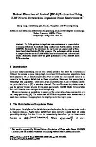
method to steer to 3.6° , 10.8° and 18.2° , respectively. Fig. 4 shows the beampattern of these three beams.
in which Pc is the number of coherent sources. It is also f L ,k
possible to do spatial smoothing based only on x (t ) or
x Lf ,k (t ) , but in this case at most M/2 coherent sources can be handled.
0 -5
1
2
x (t ) x (t ) 1
2
L
Beampattern (dB)
Thus the beamspace MUSIC algorithm may be applied to Rxfb to compute the DOA estimates of the coherent arrivals, as shown in Fig. 3. Better DOA estimation performance is expected by using the combination of beamspace MUSIC and spatial smoothing. We will show the performance comparison results in the next section via computer simulation.
R
-15 -20 -25 -30
M
-35
x (t )
-40 -90
M
Spatial smoothing,
-10
-60
fb
-30 0 30 Direction of Arrival (Deg)
60
90
x
Fig. 4. Beampattern of the three beams used for beamspace processing
Beamforming, W R W H
fb
x
4.1. Ideal Linear Array DOA estimation using beamspace MUSIC
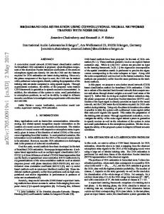
First we consider an ideal linear array. Here the ideal linear array means that there are no system errors in the array system described present. The typical spatial spectra of EMUSIC, EMUSIC-SS and BMUSIC-SS when SNR = –10dB are shown in Fig. 5. Because of the signal coherence, element space MUSIC cannot resolve the two signals, as shown by dotted line in Fig. 5. But in the same case, both EMUSIC-SS and BMUSIC-SS can resolve the two signals correctly. The advantage of the BMUSIC-SS spatial spectrum is that it has lower background and lower valley than that of EMUSIC-SS. As we know, this will help with the identification of peaks corresponding to the DOAs.
Fig 3. Combination of spatial smoothing and beamspace MUSIC to estimate DOA
4. Performance Comparison Via Computer Simulation The conventional approach to deal with the DOA estimation problem for coherent sources is combining the spatial smoothing technique and the element space MUSIC algorithm (here after we refer it to as EMUSIC-SS). We proposed to combine beamspace MUSIC and spatial smoothing (here after we denote it as BMUSIC-SS) in the previous section to achieve better DOA estimation performance. In this section, we will use computer simulation to compare these two methods.
0
EMUSIC-SS BMUSIC-SS EMUSIC
Spatial Spectrum (dB)
-10
The array used for performance comparison is a uniform linear array with M=21 sensors and half wavelength spacing. Assume there are two coherent signals having equal power incident from [10°,13°] , with respect to the broadside of the array. The signal to noise ratio is defined as 10 log 10 (var(s (t )) / σ 2 ) . The number of data sample taken at each sensor output is N=1000. To use the forward-backward spatial smoothing technique, the linear array is divided into K = 6 sub-arrays, and each sub-array has L = 16 elements. The spatial smoothed covariance matrix Rxfb can be regarded as the covariance matrix of a 16-element linear array. For this equivalent array, three beams were formed using conventional beamforming p
-20 -30 -40 -50 -60
-10
0 10 20 Direction of Arrival (Deg)
30
Fig. 5. Typical spatial spectrum of EMUSIC, EMUSIC-SS and BMUSIC-SS for ideal linear array
3
Table 1. Gain and phase errors of a practical linear array
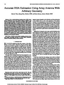
In order to compare the probability of resolution and RMSE (Root Mean Square Error) of both algorithms at different SNRs, 500 times of tests were done at each SNR from –30 to 10 dB with 2 dB step. The results were shown in Fig. 6. From Fig. 6(a), we can see that the resolution threshold of BMUSIC-SS is lower than that of EMUSICSS, and Fig. 6(b) shows that both methods have approximately the same RMSE.
element gain phase element gain phase element gain phase element gain phase
4.2. Practical Linear Array In a practical array, there will be some gain and phase uncertainty inevitably. We consider such a linear array with gain and phase errors specified in table 1. These gain and phase errors have been normalized to the first element. In this case, the typical spatial spectra of EMUSIC, EMUSIC-SS and BMUSIC-SS when SNR = –10dB are shown in Fig. 7. The element space MUSIC without spatial smoothing certainly cannot resolve the two sources, and EMUSIC-SS too fails to resolve the two sources. EMUSIC-SS BMUSIC-SS
Spatial Spectrum (dB)
Probability of Resolution
0
0.8
0.6
0.4
5 0.8 -42 10 1.17 5.37 15 1.08 6.67 20 0.89 -42.1
6 1.46 1.4 11 1.07 -32.1 16 1.15 -8.3 21 1.20 17.1
EMUSIC-SS BMUSIC-SS EMUSIC
-20 -30 -40
-60
-25
-20
-15
-10 -5 SNR (dB)
0
5
10
1.4
0.8 0.6 0.4 0.2 -20
-15
-10 -5 SNR (dB)
0
5
30
We also did 500 times of tests at each SNR from –30 to 10 dB with 2 dB step to calculate the probability of resolution and RMSE of EMUSIC-SS and BMUSIC-SS. The results were shown in Fig. 8. We see that the resolution threshold of BMUSIC-SS is still lower than that of EMUSIC-SS, but its RMSE is a little bit larger than that of EMUSIC-SS. Compared with the ideal array case, the resolution threshold of EMUSIC-SS increased due to the gain and phase uncertainty, but BMUSIC-SS can maintain its resolution threshold. It is straightforward that BMUSICSS is more robust than EMUSIC-SS, though there is a little sacrifice of its estimation accuracy.
1
-25
0 10 20 Direction of Arrival (Deg)
Only BMUSIC-SS still can resolve the two sources. This shows that BMUSIC-SS is more robust than EMUSIC-SS.
EMUSIC-SS BMUSIC-SS
1.2
-10
Fig. 7. Typical spatial spectrum of EMUSIC, EMUSIC-SS and BMUSIC-SS for practical linear array
(a) Probability of resolution
RMSE (Deg)
4 1.2 -43 9 1.21 -27.8 14 1.73 9.95 19 1.09 -16.3
-50
0.2
0 -30
3 1.16 14 8 1.11 -52 13 0.96 -32.8 18 1.14 7.7
-10
1
0 -30
2 0.65 -10.4 7 1.45 18.2 12 1.32 8.7 17 1.42 -25.6
10
5. Conclusion (b) RMSE By combining the forward-backward spatial smoothing technique and beamspace MUSIC, the DOA estimation
Fig. 6. Performance comparison of of EMUSIC, EMUSICSS and BMUSIC-SS for ideal linear array
4
Probability of Resolution
1
[3] X. L. Xu and K. M. Buckley, “A comparison of element and beam space spatial-spectrum estimation for multiple source clusters,” Proc. of Int. Conf. on Acoust., Speech, Signal Processing, pp. 2643-2646, 1990
EMUSIC-SS BMUSIC-SS
0.8
[4] H. B. Lee and M. S. Wengrovitz, “Resolution threshold of beamspace MUSIC for two closely spaced emitters,” IEEE Trans. Acoust., Speech, Signal Processing, Vol. 38, No. 9, pp. 1545-1559, September 1990
0.6
0.4
[5] P. Stoica and A. Nehorai, “Comparative performance study of element-space and beam-space MUSIC estimators,” Circuits, Systems, Signal Processing, Vol. 10, No. 3, pp. 285-292, 1991
0.2
0 -30
-25
-20
-15
-10 -5 SNR (dB)
0
5
10
[6] Y. X. Yang, Studies on beamforming and beamspace high resolution bearing estimation techniques on sonar system, Xi’an: Ph. D. thesis in Northwestern Polytechnical University, June 2002
(a) Probability of resolution 1
EMUSIC-SS BMUSIC-SS
[7] S. Haykin, Array signal processing, New Jersey: Prentice-Hall, 1985
RMSE (Deg)
0.8
[8] T-J Shan, M. Wax and T. Kailath, “On spatial smoothing for direction-of-arrival estimation of coherent signals,” IEEE Trans. Acoust., Speech, and Signal Processing, Vol 33, No. 4, pp. 806-811, April 1985
0.6
0.4
[9] S. U. Pillai and B. H. Kwon, “Forward/backward spatial smoothing techniques for coherent signal identification,” IEEE Trans. Acoust., Speech, and Signal Processing, Vol. 37, No. 1, pp. 8-15, January 1989
0.2
0 -30
-25
-20
-15
-10 -5 SNR (dB)
0
5
10
[10] J. Li, “Improving angular resolution for spatial smoothing techniques,” IEEE Trans. Signal Processing, Vol. 40, No. 12, pp. 3078-3081, December 1992
(b) RMSE Fig. 8. Performance comparison of EMUSIC, EMUSICSS and BMUSIC-SS for practical linear array
[11] J. S. Thompson, P. M. Grant, and Mulgrew, “Performance of spatial smoothing algorithm for correlated sources,” IEEE Trans. Signal Processing, Vol. 44, No. 4, pp. 1040-1046, April 1996
performance can be improved, both for ideal linear arrays and for practical arrays. Another important advantage of the method proposed in this paper is its reduced computation complexity, which will save a lot of time in the real-time system. Therefore, this method is an effective technique for real-time DOA estimation for coherent sources in practical sonar or radar systems.
[12] H. L. Van Trees, Optimum Array Processing, New York: John Wiley & Sons, Inc., 2002
References [1] R. O Schmidt, “Multiple emitter location and signal parameter estimation,” IEEE Trans. Antennas and Propagation, Vol .34, No. 3, pp. 276-280, 1986 [2] X. L. Xu and K. M. Buckley, “Statistical performance comparison of MUSIC in element-space and beam-space,” Proc. of Int. Conf. on Acoust., Speech, Signal Processing, pp. 2124-2127, 1989
5