Multiobjective Loading Pattern Optimization by Simulated Annealing ...

NUCLEAR SCIENCE AND ENGINEERING: 162, 134–147 ~2009!

Multiobjective Loading Pattern Optimization by Simulated Annealing Employing Discontinuous Penalty Function and Screening Technique Tong Kyu Park, Han Gyu Joo,* and Chang Hyo Kim Seoul National University, San 56-1 Sillim-dong, Seoul 151-744, Korea

and Hyun Chul Lee Korea Atomic Energy Research Institute, 150 Deokjin-dong, Daejeon 305-353, Korea Received April 2, 2008 Accepted December 12, 2008

Abstract – The problem of multiobjective fuel loading pattern (LP) optimization employing high-fidelity three-dimensional (3-D) models is resolved by introducing the concepts of discontinuous penalty function, dominance, and two-dimensional (2-D)–based screening into the simulated annealing (SA) algorithm. Each constraint and objective imposed on a reload LP design is transformed into a discontinuous penalty function that involves a jump to a quadratic variation at the point of the limiting value of the corresponding core characteristics parameter. It is shown that with this discontinuous form the sensitivity of the penalty coefficients is quite weak compared to the stochastic effect of SA. The feasible LPs found during SA update the set of candidate LPs through a dominance check that is done by examining multiple objectives altogether. The 2-D–based screening technique uses a precalculated database of the 2-D solution errors and is shown to be very effective in saving the SA computation time by avoiding 3-D evaluations for the unfavorable LPs that are frequently encountered in SA. Realistic applications of the proposed method to a pressurized water reactor reload LP optimization with the dual objectives of maximizing the cycle length and minimizing the radial peaking factor demonstrate that the method works quite well in practice.

I. INTRODUCTION

Therefore, satisfying all of them simultaneously can hardly be achieved, and compromises of competing objectives need to be made. For the solution of the LP optimization problem, the simulated annealing ~SA! algorithm 1 has been used widely 2– 4 because of the powerful feature of SA that prevents the solver from being trapped in local minima by allowing moves to worse states, let alone to better states. In the single-objective SA ~SOSA! algorithm, which involves only a mono-objective function, the LP optimization problem has been solved with the constrained objective function method in which the main objective function is augmented by the penalty terms reflecting the extent of violation of the constraints. The multiobjective problem involving multiple objectives has also been solved by SA algorithms.5–7 Engrand 5 was the first to present a multiobjective SA ~MOSA! algorithm,

The search for an optimum fuel assembly ~FA! loading pattern ~LP! in the reload core design amounts to a multiobjective constrained optimization problem. Given the number of fresh FAs and available burned FAs, the primary objective of the LP design in most pressurized water reactor ~PWR! reload problems is to maximize the cycle length while satisfying all safety constraints such as the maximum peak linear heat generation rate and negative moderator temperature coefficient ~MTC!. The secondary objectives would be to minimize the integrated radial peaking factor as well as the fuel cost to ensure higher thermal margin and better economy. Some of these objectives, however, are mutually exclusive. *E-mail: [email protected] 134

LOADING PATTERN OPTIMIZATION

which makes combined use of what he called the G function, which is defined as the sum of all the logarithmic values of individual objective functions, and the concept of dominance.8,9 He showed that the use of the G function for calculating the acceptance probability of trial solutions and the concept of dominance 8 for archiving candidate solutions enable his MOSAto find the surface of Pareto points or the trade-off surface that multiobjective optimization solvers seek. Parks and Suppapitnarm 6 noted that Engrand’s MOSA algorithm has two weaknesses such as the possibility of favoring some objectives over others and that of discriminating trial solutions moving toward the trade-off surface. Pointing out that these weaknesses are attributed to the dissimilarity in magnitude of individual objective functions forming the G function and a deficiency of the acceptance logic of trial solutions, they suggested an improved MOSA algorithm that uses individual annealing temperatures for each objective instead of the composite objective function like Engrand’s G function and a modified acceptance logic. In their acceptance logic, an archiving for the trial solution and then the routine SA acceptance test is followed for the failed LPs. Keller 7 observed that the improved MOSA algorithm 6 has several drawbacks when applied to constrained in-core optimization problems with a large number of constraints. Their formula to calculate the acceptance probability as the product of individual acceptance probabilities is apt to cause arithmetic underflow or overflow errors when a new LP accompanies a large change in one of the objective function values. The individual annealing schedule for each objective may lead to premature cooling with the increasing number of objective functions, which would either cause trapping in local minima when the optimization proceeds with an LP far from the trade-off surface or not allow a search length adequate to characterize a trade-off surface in the presence of constraints. Keller 7 showed that he could get around three drawbacks by introducing several modifications in the formula for acceptance probability calculation, annealing rate parameters for individual objectives, annealing schedule for the primary objectives, adaptive penalty control algorithm, a termination criterion, etc., at the cost of complexity and empiricism. As noted from these developments, one of the central elements that characterize a MOSA algorithm is how to determine the acceptance probability of a new trial solution along with the annealing schedule. Using the G function as if it were a composite objective function is the salient feature of Engrand’s MOSA, even though the G function is the source of its weakness. The improved MOSA ~Refs. 6 and 7! avoids the G function because of its deficiency by using individual annealing temperatures for each objective. Formulating the composite objective function adequately, however, one can devise another MOSA algorithm that gets around not only the weaknesses of Engrand’s MOSA but also the complexity and empiricism of the improved MOSA. NUCLEAR SCIENCE AND ENGINEERING

VOL. 162

JUNE 2009

135

One of the objectives of this paper is to present a new MOSA algorithm that utilizes a discontinuous penalty function as the composite objective function fit for a given multiobjective optimization problem. The new MOSA is similar to Engrand’s because it uses the composite objective function to determine the acceptance probability of trial solutions, yet it does not have the shortcoming of the latter because individual objective functions forming the composite objective function are similar in magnitude. The new MOSA is different from Engrand’s because it treats the composite objective function just like the constrained objective function of SOSA optimization problems. As a consequence, the parallel computing SOSA algorithm available in Ref. 4 can be implemented automatically without complexity and empiricism 7 introduced by Keller for the efficacy of the improved MOSA. Specifically, the new MOSA is free from the possibility of committing underflow or overflow errors. It does not need adaptive penalty control measures to avoid the constraint violation of the archive solutions because discontinuous penalty functions are used to construct the composite objective function. It does not require introducing the two-stage annealing schedule for the primary objectives to promote the SA search along the trade-off surface. The termination criterion as well as the cooling rate parameters do not rely on empiricism. These points will be discussed in Sec. II. In contrast to the merit of a better global minimum search capability, a drawback of SA is the huge computing requirement leading to a long execution time. One of the measures that can be used to reduce the computing time is parallelization, and the other would be to use a lower-order model.10 In the previous work,4 we proposed a parallel computing adaptive SA scheme employing a two-dimensional ~2-D! core model. However, it is often encountered that the final solution obtained from the 2-D model–based SA calculation is not satisfactory when it is reevaluated by the three-dimensional ~3-D! model. In order to avoid this problem, it is better to adopt the 3-D model being used in the design analysis directly during the SA calculation although this will lead to a significant increase in the computing time. However, it is possible to establish an efficient 3-D model–based SA scheme that can avoid excessive 3-D evaluations by utilizing a 2-D model–assisted acceptance or rejection criterion. As the second objective of this paper, we present a 2-D model–based screening technique 11,12 ~ST! that allows a considerable portion of the LP evaluation done by a 2-D model rather than by a 3-D model. In order to assess the performance of the new MOSA-based LP optimization method characterized by both the discontinuous penalty function and the 2-D–based ST, the LP optimization problem of a real PWR plant, cycle 4 of Yonggwang Nuclear Unit 4 ~YGN4! of Korea,13 is solved with the dual objectives of maximizing the cycle length and minimizing the radial peaking factor.

136

PARK et al.

II. MULTIOBJECTIVE SIMULATED ANNEALING WITH DISCONTINUOUS PENALTY FUNCTIONS

The optimization problem stated by Eq. ~1! is then rephrased in this method as Find X that minimizes F~X ! .

The LP optimization problem here is to find the best FA LP for a reload cycle PWR core that maximizes the cycle length and minimizes the power peaking factor as well as the fuel cost while meeting all the design constraints. It is thus a constrained optimization problem. Mathematically, the problem can be stated as follows: Find X that minimizes f~X ! subject to g~X ! ⱕ 0 , ~1! where X designates an LP. f~X ! ⫽ @ f1 ~X !, . . . , fm ~X !# T is an m-dimensional column vector with the superscript T denoting the transpose of a vector. fi ’s ~i ⫽ 1, 2, . . . , m! are individual objective functions to be minimized individually and are associated with the cycle length, the peaking factors, and other performance parameters of LP X. g~X ! ⫽ @ g1 ~X !, . . . , gn ~X !# T is an n-dimensional column vector formed by n design constraint functions, gj ~ j ⫽ 1, 2, . . . , n!. For our problem, the design constraints generally include the limits for the radial pin power peaking factor ~Fr !, the peak linear heat rate or the 3-D pin power peaking factor ~Fq !, the pin discharge burnup ~PDB!, the MTC at hot full power and at hot zero power at beginning of cycle, etc. In order to solve the minimization problem by SA, it is necessary to define a scalar functional in terms of the multiobjective functions and constraint functions. In the following, several methods for defining the scalar functional are discussed starting from the conventional penalty function method.14 The goal is to establish a new multiobjective function that can be less sensitive to the penalty coefficients.

The vector u or the penalty coefficients are fixed constants in the static penalty function method while they may change adaptively in the dynamic penalty function method during the course of SA optimization calculations. In either case, the determination of the proper u is a difficult problem because the relative weight of any one constraint function to another constraint function can hardly be known. Actually, how to set the penalty coefficients for all the involved constraint functions is not a well-defined problem either. Besides, there is no 100% guarantee that the optimum solution from it does not violate the constraints all the time, unless u is carefully controlled. Because of these reasons, it is desirable to convert the constrained minimization problem to an unconstrained problem that does not require determining penalty coefficients. Suppose that the design constraints are given by ai ~X ! ⱕ ailim ,

i ⫽ 1, 2, . . . , n .

~4!

Let us define the penalty function, Ji ~X ! ~i ⫽1, 2, . . . , n!, corresponding to each constraint by

冉

Ji ~X ! ⫽ a i ⫹

di ~X ! 2 di2

冊

u~di ~X !! ,

~5!

where di ~X ! ⫽ ai ~X ! ⫺ ailim , di2 ⫽

1

N

( di ~Xk ! 2 u~di ~Xk !! N k⫽1

,

and a i is a user-defined constant that may be taken simply to 1. u~ x! is the unit step function defined as

II.A. Formulation of Discontinuous Penalty Function The penalty function method treats design constraints as penalty terms on the optimization functional that is to be minimized. As such it makes use of the scalar functional F~X ! defined as a weighted sum of individual objective functions: F~X ! ⫽ w T f~X ! ⫹ u T g~X ! ,

~3!

~2!

where w ⫽ @w1 , . . . , wm # T ⫽ m-dimensional column vector consisting of m weighting factors, v i ~i ⫽ 1, 2, . . . , m! u ⫽ @u1 , . . . , un # T ⫽ n-dimensional column vector consisting of n penalty coefficients, uj ~ j ⫽ 1, 2, . . . , n!.

u~ x! ⫽

再

1 ,

x⬎0

0 ,

xⱕ0 .

~6!

di ~X ! is the deviation of the i ’th constraint of a given LP X. di2 is the expected value of the squared deviation of the i ’th constraint. It is used here to normalize the value of di2 so that Ji ~X ! becomes more or less similar in magnitude regardless of the types of constraints. Note that u~di ~X !! and Ji ~X ! are 0 if LP X satisfies the constraint, Eq. ~4!, and they are nonzero otherwise. Thus, Ji ~X ! has a discontinuity at the limiting value, ai ~X ! ⫽ ailim , and becomes a quadratic function of ai ~X ! beyond this limit. The penalty function given by Eq. ~2! can be extended to the individual objective functions as well by lim setting ak⫹n as the required maximum for the k’th objective function. For example, it can be the maximum pin NUCLEAR SCIENCE AND ENGINEERING

VOL. 162

JUNE 2009


peaking factor for the reload core. In this way, one can treat the m objectives in exactly the same way as n constraints. Now, let us define a global penalty function as the summation of all the penalty functions representative of n constraints and m objective functions: m⫹n

J ~X ! ⫽

( Ji ~X !

.

~7!

i⫽1

The combination of this global penalty function with the original objective functions can convert the constrained minimization problem into an unconstrained one, which may be stated as follows: Find X that minimizes F~X ! ⫽ @J ~X !, f1 ~X !, . . . , fm ~X !# T .

~8!

Note that the minimum value of J ~X ! is zero. Therefore, any LP X satisfying J ~X ! ⫽ 0 not only meets all the constraints but also guarantees that each individual objective function is less than the required maximum set individually. This means that LP X satisfying J ~X ! ⫽ 0 is qualified as a solution of our optimization problem, and therefore, it is called the feasible solution. Our new MOSA takes advantage of this fact. The global penalty function is viewed as the composite objective function to be minimized and is treated just like the constrained objective function of the SOSA optimization problem in the new MOSA. Consequently, the MOSA solution can be obtained by a routine SOSA algorithm with 4 or without 2,3 parallel computing arrangements. The new MOSA seeks the optimum LP through repeated applications of the three-step SA algorithm: 1. creation of a new LP, X new , from the current LP, X cur 2. comparison of the objective function values of the current and the new LPs, J ~X cur ! and J ~X new ! 3. acceptance of X new with the acceptance probability of exp~⫺DJ0C!, where DJ ⫽ J ~X new ! ⫺ J ~Xcur ! and C represents the cooling temperature. At the end of the SA calculation, there may be one or more feasible LPs satisfying J ~X ! ⫽ 0. If this is the case, the best LP can be chosen among the feasible LPs listed in the order of importance of the designer-set main objective. In case that no feasible LP is produced, one may repeat the SA calculation with some adjustment of the SA parameters involved, such as the cooling rate, the number of LPs being sampled at each cooling stage, or the limits set for the main objective functions. The SOSA algorithm employed for the new MOSA has a serious shortcoming in that it lacks a recipe for recognizing the superiority of one feasible LP over the other feasible ones when determining acceptance of X new because X new is always accepted once it is a feasible LP, namely, when J ~X new ! ⫽ 0. As a result, discriminating NUCLEAR SCIENCE AND ENGINEERING

VOL. 162

JUNE 2009

137

the inferior feasible LP against the superior feasible LP and intervening in the acceptance or rejection of the new LP is not possible with the J function only. To overcome this shortcoming, we incorporate the concept of dominance,8 which has been used in the multiobjective genetic algorithm 9 and also in the existing MOSA algorithms.5–7 The definition is available in the literature. For clarity of our new MOSA algorithm, it is defined here again at the risk of repetition. Suppose that two LPs X 1 and X 2 are feasible. X 1 is said to dominate X 2 if all the objective functions of X 1 are smaller than those of X 2 , namely, if fi ~X 1 ! ⬍ fi ~X 2 ! for all i. Thus, a dominating LP is the better of the two LPs from the standpoint of the objectives of the LP optimization. Incorporation of the concept of dominance into the SA algorithm enables one to accept a new feasible LP when it dominates the current feasible LP that has produced it and makes it possible to remove those feasible LPs archived as the candidate feasible LP set ~simply the candidate LP set hereafter! if they are dominated by the new feasible LP. The candidate LP set here refers to the set of the feasible LPs that are created and updated through the dominance check during the course of MOSA optimization. The logic for updating the candidate LP set is explained below together with the acceptance logic for the new LP. Figure 1 shows the SA acceptance algorithm modified by incorporating the concept of dominance. As noted in Fig. 1, the conventional SA algorithm is basically applied, but it is subject to modification when a new feasible LP is produced from the current feasible LP. Suppose that a feasible LP X new is generated from X cur , i.e., J ~X new ! ⫽ 0. If X cur is not a feasible LP, i.e., if J ~X cur ! ⫽ 0, X new is automatically accepted, and a dominance check is made with the members of the candidate LP set. If X cur is already a feasible one, however, X new is accepted only when it meets dominance conditions dictated by the modified SA algorithm. First of all, X new is always accepted if it dominates X cur . Otherwise, dominance checks are made to determine ~a! whether X new dominates any member of the existing candidate LP set or ~b! whether X new and the existing candidate LPs are not dominated mutually. If these are the cases, X new is accepted and registered as a new member of the candidate LP set. Otherwise, it is rejected. It must be noted that any existing candidate LPs dominated by X new are eliminated from the candidate LP set whenever the feasible X new is accepted. Besides the acceptance logic of the feasible X new , the new MOSA algorithm is distinguished from the SOSA algorithm in that the former eliminates those member LPs of the existing candidate LP set that are dominated by the newly accepted feasible LP, while the latter retains all the new feasible LPs as the member of the candidate LP set. The new MOSA algorithm updates the candidate LP set at every acceptance of a new feasible LP. After the search is completed, the resulting candidate

138

PARK et al.

Fig. 1. Acceptance logic of the new MOSA algorithm.

LP set will contain the feasible LPs that are mutually nondominating but dominate all the other feasible LPs that have been generated during the SA calculation. The designer can choose one of them as the final solution, namely, the best LP. In summary, incorporation of the concept of dominance into the SA algorithm affects the LP search calculations in two ways. One is to fill gradually the candidate LP set by better LPs dominating the previous feasible LPs. Another is to affect the LP search calculation itself by rejecting the feasible new LPs that are dominated by any existing candidate LP. The effect is nonexistent in the conventional SA calculation and stands out at the later stage of SA calculation when the cooling temperature is very low and it is highly likely to generate new feasible LPs from the current feasible LP. Needless to mention, when the feasible X cur registered as a member in the candidate LP set produces a nonfeasible X new , this has the chance of being accepted as dictated by the SA acceptance probability and may induce a move toward a feasible LP or the trade-off surface according to the subsequent applications of the MOSA algorithm. The penalty function defined by a weighted sum of discontinuous penalty functions given in Eq. ~7! has an advantage that its minimum value is always zero irrespective of the weighting factors. Obviously, it is a special case of the general penalty function, n⫹m

JD ~X ! ⫽

( wi Ji ~X ! i⫽1

,

~9!

which has the minimum value of zero, for any set of wi ’s Note that Eq. ~7! is obtained with uniform weights, e.g.,

wi ⫽ 1 for all i. For this reason, the use of the uniformly weighted penalty function, Eq. ~7!, with the penalty functions modified slightly from those in Eq. ~5!,

冉

Ji ~X ! ⫽ 1 ⫹ cI i

di ~X ! 2 di2

冊

u~di ~X !! ,

~10!

can produce the same result as the nonuniformly weighted penalty function given by Eq. ~9!. In this context, let us note that cI i plays a similar role as the relative importance of the constraint function or the objective function. To be able to apply the SA algorithm for minimization of the penalty function discussed above, one should specify constants cI i and di2 in Eq. ~10!. By definition, determination of di2 requires sampling all the possible LPs. In practice, however, it is inevitable to use an average value 2 of di2 over a finite sampling of LPs, say, diN , which is an 2 average value of di obtained from N LPs sampled initially. There must be the discrepancy between di2 and 2 2 2 2 diN by DdiN ⫽ di2 ⫺ diN . In terms of diN the penalty function given by Eq. ~10! can be rewritten as

冉

Ji ~X ! ⫽ 1 ⫹ ci

di ~X ! 2 2 diN

冊

u~di ~X !! ,

~11!

where ci ⫽

2 diN 2 2 diN ⫹ DdiN

NUCLEAR SCIENCE AND ENGINEERING

cI i . VOL. 162

JUNE 2009


Since cI i is a user-specified constant representing the relative importance of the i ’th constraint, ci is also regarded as a free parameter. For the sake of interest, however, it will be shown later that the SA optimization process has a weak dependence on ci . Thus, it does not really matter what value to use for ci in the new MOSA optimization formulation based on the discontinuous penalty function. II.B. Two-Objective Loading Pattern Optimization The multiobjective optimization formulation presented above is applicable to problems of both multiple objectives with m . 1 and a single objective with m ⫽ 1. To illustrate the simplest example of the multiobjective optimization formulation and also to examine the viability of the MOSA algorithm incorporating the concept of dominance as well as the penalty function method, we consider the reload design problem of the cycle 4 core of YGN4 as the dual-objective LP optimization problem aiming at finding the best LP to have the longest cycle length ~L c ! and the lowest possible radial peaking factor ~Fr !, given the fresh and once- and twice-burned FAs. The choice of the lowest Fr as another objective parameter here is intended to secure the thermal margin as large as possible because it can turn into an economic benefit. Table I lists the parameters of both the design constraints and the objectives. Fr usually plays as a design constraint, particularly in the single-objective optimization problem, but it is treated here as one of the objective parameters. Representing the cycle length to be maximized in the form like constraints, namely, Eq. ~4!, in conformity with the penalty function method needs a little precaution. Because the penalty function method is designed to minimize the involved objective parameters, one treats here the negative value of the cycle length as the objective parameter. The constrained optimization condition that the cycle length should meet the required minimum cycle length ~L c,min !, e.g., L c ~X ! ⱖ L c,min , can be expressed equivalently as ⫺L c ~X ! ⱕ ⫺L c, min .

~12!

139

The dual-objective minimization problem is then stated as follows: Find X that minimizes F~X ! ⫽ @J ~X !,⫺L C ~X !, Fr ~X !# T .

J ~X ! in the three-element objective function vector F~X ! is given in Eq. ~7! with the individual penalty functions Ji ~X ! defined in Eq. ~11!.

III. SCREENING TECHNIQUE ASSISTED BY TWO-DIMENSIONAL NEUTRONICS EVALUATION MODEL

As mentioned in Sec. I, the SA optimization has a major drawback of long computing time because it requires evaluation of tens of thousands of trial LPs. To get around this, one is tempted to adopt simpler and faster evaluation models such as 2-D models,2 neural network– assisted models, etc.10 In most cases, however, the best LPs from these simplified models turn out to be far from being optimal when they are reevaluated by the 3-D design code. To serve the reload core designers’ needs, it is most desirable to adopt the 3-D core model used for the neutronic design. The issue in this case is how to alleviate the computational burden. The ST is a way to resolve this issue by screening out a considerable portion of 3-D evaluation of trial LPs and thus reducing the SA computation time. The ST takes advantage of a predetermined distribution function on dJ ~X ! ⫽ J 3-D ~X ! ⫺ J 2-D ~X !, the difference between the 3-D constrained objective function, J 3-D ~X !, and its 2-D counterpart, J 2-D ~X !, for X. To obtain the distribution function for dJ ~X !, one needs to sample and evaluate a set of LPs that supposedly represent the whole range of LPs subject to the SA optimization calculation. Suppose that one has obtained the distribution with the mean dJ and the standard deviation s and also ek ⫽ Pr $6dJ ~X ! ⫺ dJ6 ⱕ ks%, which is the probability of dJ ~X ! lying within 6ks ~k ⫽ 1, 2,

TABLE I Design Constraints and Objectives for Cycle 4 Core of YGN4 i

Symbol ai

Design Parameters

Design Limit

Target Limit

1 2 3 4 5 6

Fr Fq BD aZ aF LC

Integrated radial pin peaking factor 3-D pin peaking factor Pin discharge burnup ~GWd0tonne U! Hot zero power MTC ~pcm08C! Hot full power MTC ~pcm08C! Cycle length ~effective full-power day!

1.55 2.58 54 5 0 383

1.50 2.20 54 5 0 393


VOL. 162

JUNE 2009

~13!

140

PARK et al.

3-D or 3! from dJ. If one defines Jmax ~X ! ⫽ J 2-D ~X ! ⫹ dJ ⫹ 3-D 2-D ks and Jmin ~X ! ⫽ J ~X ! ⫹ dJ ⫺ ks, it follows that 3-D the probability of J 3-D ~X ! lying between Jmin ~X ! and 3-D Jmax ~X ! is 100ek %, namely, 3-D 3-D ⱕ J 3-D ~X ! ⱕ Jmax ! ⫽ 100ek% Pr~Jmin

~14!

or 3-D 3-D Pr~J 3-D ~X ! ⬍ Jmin or J 3-D ~X ! ⬎ Jmax ! ⫽ 100~1 ⫺ ek !% .

~15! The value of ek depends on the actual distribution function of dJ ~X ! and the k value. For example, e2 ⫽ 0.956 and e3 ⫽ 0.997 in the case that dJ ~X ! is normally distributed. If one uses e2 in Eq. ~15! in this case, one sees 3-D 3-D that Pr~J 3-D ~X ! ⬍ Jmin ! or Pr~J 3-D ~X ! ⬎ Jmax ! is only 2.2% because of the symmetry of the normal distribution. The ST makes the most of this result to devise an approximate acceptance or rejection criterion that does not require 3-D evaluation for a trial LP sampled in the course of SA optimization. In order to show how the ST works, let us consider the acceptance probability of a new LP X new produced from the current LP, X cur , exp~⫺DJ0C!. In the SA calculation, this probability is simulated by the pseudorandom number j, and X new is either accepted when exp~⫺DJ0C! ⱕ j or rejected when exp~⫺DJ0C! ⬎ j. Note that the acceptance and the rejection criteria can be rewritten as SA criteria ⫽

再

X new is accepted if J ~X new ! ⱕ J ~X cur ! ⫺ C ln j X new is rejected if J ~X new ! ⬎ J ~X cur ! ⫺ C ln j .

~16! Obviously, 3-D evaluation of the penalty functions of all the LPs to be tested by the SA criteria above is costly. As a way to avoid the necessary 3-D evaluation for J ~X new !, 3-D the ST uses Jmax ~X new ! to implement the acceptance cri3-D terion while it uses Jmin ~X new ! to implement the rejection criterion. Instead of Eq. ~16!, the ST accepts X new without 3-D calculation when the following condition is satisfied: 3-D Jmax ~X new ! ⬍ J ~X cur ! ⫺ C ln j ,

~17a!

3-D ~X new ! ⫽ J 2-D ~X new ! ⫹ dJ ⫹ ks . Jmax

~17b!

where

On the other hand, the ST rejects X new without 3-D calculation when the following condition is met:

3-D Jmin ~X new ! ⬎ J ~X cur ! ⫺ C ln j ,

~18a!

3-D Jmin ~X new ! ⫽ J 2-D ~X new ! ⫹ DJ ⫺ ks .

~18b!

where

The acceptance criterion, Eq. ~17!, and the rejection criterion, Eq. ~18!, require only the 2-D evaluation of X new . If X new meets Eq. ~17!, it is accepted without the 3-D evaluation for it. Likewise, if X new satisfies Eq. ~18!, it is rejected without the 3-D evaluation for it. In other words, the above criteria screen out the 3-D evaluations for some of the trial LPs that may appear in the SA optimization process. Consequently, they can reduce the SA computing time. We observe that the acceptance criterion screens out effectively the 3-D evaluations of the trial LPs at the earlier stages of the SA algorithm when the cooling temperature C is high, while the rejection criterion does at the later stages of the SA algorithm when the cooling temperature C is low. Note that the acceptance probability of X new at the high-temperature earlier stages of SA is close to 1, and thus, a greater portion of LPs sampled are accepted as X new , while the rejection probability of X new at the low-temperature later stages of SA is close to 1, and thus, a greater portion of LPs sampled are rejected. As a matter of course, when X new is accepted by Eq. ~17!, it replaces X cur as the SA algorithm dictates. Unless the penalty function value of X new is too low, e.g., ⬍Jlim , it is approximated by J 3-D ~X new ! ⬇ JD ~X new ! ⫽ J 2-D ~X new ! ⫹ dJ. On the contrary, if JD ~X new ! ⬍ Jlim , a 3-D calculation is performed to determine J 3-D ~X new ! more accurately. The decision on acceptance of X new in this case is made once more according to the normal acceptance criterion for three dimensions, Eq. ~17!. The algorithm of screening as well as the dominance check explained so far is given in a pseudocode form in Fig. 2. The adoption of the ST may have an unspecified effect on the best LP search process by the SA algorithm by probably accepting or rejecting LPs that could not be accepted or rejected if the 3-D model is used to evaluate them. In order to avoid this effect as far as one can, one may set ek as high as practicable so that 3-D 3-D Pr~J 3-D ~X ! ⬍ Jmin ! or Pr~J 3-D ~X ! ⬎ Jmax ! becomes small enough to justify the use of the modified acceptance and rejection criteria, Eqs. ~15! and ~16!, with high confidence. Considering that the increasingly higher ek results in increasingly higher confidence, but increasingly lower efficiency, of the ST, we here adopt e2 ⫽ 0.954 as a compromise. e2 ⫽ 0.954 can be derived exactly when the normal distribution is assumed for dJ ~X !. It is arbitrarily set here regardless of the actual distribution function for dJ ~X !. It must be noted that utilization of Eqs. ~14!, ~15!, or ~16! for the ST does not need the distribution function for dJ ~X ! but the numerical value for ek . NUCLEAR SCIENCE AND ENGINEERING

VOL. 162

JUNE 2009


141

mance of which will be compared with the optimum or the near-optimum LPs generated from the MOSA algorithm presented above. The FAs designated by G0, G1, and G2 are fresh assemblies with 0, 8, 12 burnable poison rods ~BPRs!, respectively, while the remaining FAs are once- and twice-burned ones. Table I shows the design limits and constraints actually used for the reference LP and the target limits imposed in this study. IV.A. Input Parameters of New Multiobjective Simulated Annealing Algorithm and Neutronics Evaluation

Fig. 2. Pseudocode for SA with dominance check and screening.

IV. APPLICATION TO REALISTIC LOADING PATTERN SEARCH

The new MOSA algorithm with the discontinuous penalty function and the 2-D–based ST described above were implemented in the Unified Nodal Code for Advanced Reactor Design and Simulation 15 ~UNCARDS!. To examine its effectiveness in a realistic LP search problem, UNCARDS is applied for the reload design of the cycle 4 core of YGN4, which is a former CombustionEngineering PWR loaded with 177 FAs ~Ref. 13!. Shown in Fig. 3 is the actual FA LP for the cycle 4 core of YGN4. It is taken here as the reference LP, the perfor-

The new MOSA algorithm requires user-specified input parameters such as the initial acceptance ratio x, the number of LPs generated and accepted per stage Nsmp and Nacp , the stopping criterion «s , and the probabilities of generating new LP generation logics from a current LP; binary exchanges of FAs ~P1 !, addition of BPRs in fresh FAs ~P2 !, and rotation ~P3 !. Typical values for these parameters have been suggested in previous work.4 The same values of 0.99, 500, and 50 are used here for x, Nsmp , and Nacp , respectively. «s is set to 0.001, while P1 , P2 , and P3 are set to 0.7, 0.3, and 0.0, respectively. In addition to these parameters, the param2 eters such as mean squared deviation diN and the relative penalty importance parameters ci and Jlim need 2 to be set. Since diN can be determined only through evaluations of a certain number of LPs, 100 LPs are 2 arbitrarily generated initially to determine diN . The specification of ci ’s requires care because they determine the relative contribution of the individual penalty functions to the overall penalty function and thus may affect the result of the MOSA optimization. After an extensive sensitivity analysis to be discussed in Sec. IV.B, they are all set to 1.0. Jlim can affect the screening efficiency, if it is set to an unnecessarily high value. In this study, it is set to 2. The 3-D evaluation of LPs by UNCARDS is performed with four radial nodes per FA and 26 axial nodes, while the 2-D evaluations are conducted with one node per assembly. The number of burnup steps is 15. The cycle length is measured in the core average cycle burnup in MWd0kg at the end of the cycle, namely, when the critical soluble boron concentration reaches 10 ppm. IV.B. Sensitivity Analysis

Fig. 3. Reference fuel LP of cycle 4 core of YGN4. NUCLEAR SCIENCE AND ENGINEERING

VOL. 162

JUNE 2009

In the discontinuous penalty function method presented in Sec. II, the penalty coefficients ci ’s are free parameters that must be specified for the MOSA calculations. In order to determine these coefficients properly, the sensitivity of MOSA optimization results to these values needs to be examined first. Among the six coefficients, c1 and c6 are chosen for the sensitivity analysis because of the following reasons. First, they are the

142

PARK et al.

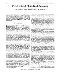
penalty coefficients related directly to the dual objectives in this study and therefore are considered more important than the others. Second, the MTC and PDB constraints can be readily satisfied whereas the peaking and cycle length constraints are more difficult to meet. Third, the 3-D peaking factor and radial peaking factor are interrelated. For the required sensitivity analysis, four different values are assigned to each penalty coefficient, which comes up with 16 different cases in terms of the pair of values for ~c1 , c6 ! as listed in Table II. For the application of the ST, the probability parameter e2 is arbitrarily set to 0.954. This implies that the probability that dJ is within the 2s ranges around dJ is 95.4% no matter which distribution dJ may actually assume. To validate this, we calculated dJ for about 3000 independent LPs for each case of Table II and examined the fraction of LPs whose dJ value is within dJ 6 2s. As shown in Fig. 4, the fraction of LPs whose dJ is within the 2s ranges of dJ turns out to be .95.4% for all 16 cases. Thus, this ensures that the lower and upper bounds of dJ given by Eq. ~14! are met.

TABLE II A Pair of Parameters ~c1 , c6 ! for Sensitivity Analysis by Case Number c6 c1

0.1

1

10

100

0.1 1 10 100

1 5 9 13

2 6 10 14

3 7 11 15

4 8 12 16

For each of the 16 cases, the dual-objective LP optimization calculations are performed, and 16 sets of the final candidate LPs are obtained as summarized in Table III, which lists the number of LP’s sampled ~Ngen !, the number of LPs subject to 3-D evaluations ~N3-D !, the number of LPs accepted ~Na !, the screening efficiency ~hST !, the number of feasible LPs ~Nfea !, the number of candidate LPs ~Ncan !, and the turnaround time ~Thr !. It is observed that all the LPs in the final candidate set satisfy all the design constraints imposed: namely, the values of the penalty function are all zero, and only those LPs that are nondominating mutually remain in the final candidate set. The screening efficiency turns out to range from 51 to 74%, and the turnaround time varies from 6.8 to 13 h on a Linux cluster consisting of 35 Xeon CPUs ~eleven 3.0-GHz Xeon 3.0 CPUs and twenty-four 2.33-GHz Xeon 64 CPUs!. A final candidate LP set is always produced for each of the 16 cases although the number of LPs in each candidate set differs depending on the cases. For further examination, the L c ⫺ Fr plots of all the LPs in the 16 candidate sets are shown in Fig. 5. From comparison of the candidate LP sets in terms of the cycle length and the peaking factor of the individual LPs, it seems that cases 7, 11, or 12 give rise to better LPs while case 10 has worse LPs than those in any other candidate sets. The better LPs here refer to those that have relatively longer cycle lengths but relatively lower peaking factors and are located in the lower right region of Fig. 5. By observing that c1 ⫽ 1 and c6 ⫽ 10 for the best case ~case 7! and c1 ⫽ 10 and c6 ⫽ 1 for the worst case ~case 10!, one may conjecture that the penalty coefficients may affect the optimum results of the dualobjective SA calculations. To ascertain whether this is a

TABLE III Summary of MOSA Optimization for the 16 Cases for the YGN4 Cycle 4

Fig. 4. Fraction of LPs whose dJ’s are within 2s ranges around dJ.

Case

Ngen

N3-D

Na

hST

Nfea

Ncan

Th

1 2 3 4 5 6 7 8 9 10 11 12 13 14 15 16

15 881 11 222 11 099 15 240 12 233 13 854 10 112 15 783 11 376 15 881 13 524 16 289 13 162 19 605 17 476 14 703

6763 3959 5451 4465 4058 4697 4506 5228 4580 4193 6078 5936 5044 5277 7878 6333

4203 2980 3493 2968 3247 3081 3320 3245 3281 3060 2998 3422 3114 3423 3370 3402

0.57 0.65 0.51 0.71 0.67 0.66 0.55 0.67 0.60 0.74 0.55 0.64 0.62 0.73 0.55 0.57

565 496 341 402 548 293 216 372 288 448 353 282 399 915 320 269

6 8 1 2 3 6 6 1 1 5 2 5 2 11 4 1

11.4 6.8 9.1 7.7 7.1 7.8 7.8 8.7 7.9 7.0 10.3 10.1 8.8 8.2 13.0 10.8


VOL. 162

JUNE 2009


Fig. 5. L C -Fr plot of LPs in the final candidate sets from 16 different cases in ~c1 , c6 !.

pure coincidence or a real trend, the SA optimization calculations for cases 7 and 10 are redone by employing different random number sequences because the stochastic effect resulting from different random numbers may affect the SA outcome. Twelve candidate sets or a total of 55 candidate LPs are obtained from six independent SA runs for each of cases 7 and 10, including the two original sets shown already in Fig. 5. Figure 6 shows the L c ⫺ Fr plots of the 55 LPs in the 12 candidate sets. The L c ⫺ Fr plots show that in contrast to the observation in Fig. 5, case 7 can generate worse candidate LPs while case 10 can produce better candidate LPs comparable to those plotted for this case in Fig. 5, depending on the

Fig. 6. L C -Fr plot of LPs in 12 final candidate sets from 12 independent runs for cases 7 and 10. NUCLEAR SCIENCE AND ENGINEERING

VOL. 162

JUNE 2009

143

Fig. 7. Behavior of discontinuous penalty function with different ci .

random number sequence. This indicates clearly that the outcome of the dual-objective SA optimization depends less on the values of the penalty coefficients represented here by c1 and c6 but rather strongly on the stochastic effect. The weak dependence on the penalty coefficients can be better explained by using Fig. 7, which illustrates the dependence of the discontinuous penalty function J ~X ! on one of the penalty coefficients ci . The three curves in Fig. 7 are obtained with the three different ci values, but they share the same discontinuity point and the same horizontal line below this point. Consider now two LPs, a feasible LP X, and a nonfeasible LP X ' . The discontinuous penalty function value of X is always zero regardless of the value of ci while that of X ' is 3, 5, and 9, respectively, for the three different ci values. Obviously, the acceptance probability of new LPs above the nonfeasible region depends on ci values. Therefore, the moves from a nonfeasible LP like X ' to another nonfeasible LP are affected by ci values. The effect depends on where the moves occur and becomes increasingly weaker as the region of moves approaches the feasible region. Suppose now that X is produced as a new LP from X ' in the course of the MOSA calculation. This is the move that reduces the discontinuous function value. Though the magnitude of reduction in the discontinuous function values depends on the ci value, X is always accepted, regardless of the ci values. Once X is produced, the acceptance probabilities for the moves from X to other feasible LPs around X are not affected because the moves do not change the discontinuous penalty function values no matter what values ci may have. Only the stochastic effect is dominant in the feasible region and can lead the search to the nonfeasible region. Although the value of ci can affect the path leading to the feasible region, it is not very significant unless the feasible region is very narrow. Finer tuning in the feasible region is performed

144

PARK et al.

stochastically by dominance check. This is the merit of the new MOSA algorithm based on the discontinuous penalty function and dominance check. IV.C. Optimization Calculation for Cycle 4 Core of YGN4 With all the necessary input parameters for the MOSA algorithm as specified above, ten independent MOSA optimization runs are conducted. Each MOSA run is done with different random number sequences to examine the stochastic effect. The results are summarized in Table IV. From the results of ten MOSA runs, it is estimated that the average CPU time is ;8.1 h. The average screening efficiency is ;66% with approximately 95 770 LPs out of approximately 144 000 LPs generated in ten MOSA runs screened out. On the ten-run average, a total of 372 LPs out of 14 400 LPs are found to be feasible solutions; among them 5 remain as candidate LPs. Actually, the ten optimization runs produced a total of 54 candidate LPs, which are displayed in L c ⫺ Fr plots in Fig. 8. From an additional dominance check over them, five final candidate LPs are finally obtained. Shown in Table V are the core performance parameters of the 15 candidate LPs selected by the order of cycle length. It should be noted that all the final five LPs are included in Table V and that they are better than the reference one in that the cycle length is longer by .20 days while the peaking is lower by .2.5%. Surprisingly though, it turns out that all of the five final candidate LPs are produced from the third SA run. Figure 9 displays the number of the feasible LPs and that of candidate LPs in the candidate LP set as a function of the stage number of the third optimization run. Figure 10 illustrates the evolution of the candidate LP set with the progress of the stages. The first candidate

TABLE IV Summary of Ten Optimization Runs for Cycle 4 Core of YGN4 Run

Ngen

N3-D

Na

hST

Nfea

Ncan

Th

1 2 3 4 5 6 7 8 9 10

17 236 11 398 10 888 17 694 13 982 12 600 12 401 14 393 17 155 16 249

5 959 4 089 3 427 4 668 4 882 4 136 5 231 5 210 4 949 5 676

3 654 3 155 2 649 2 918 3 352 3 209 3 183 3 470 3 374 3 696

0.65 0.64 0.69 0.74 0.65 0.67 0.58 0.64 0.71 0.65

424 502 445 411 400 348 315 304 366 208

5 6 5 5 7 7 6 4 5 4

9.5 6.9 5.8 7.7 8.0 7.3 8.8 8.6 8.5 9.8

Total

143 996

48 227

32 660

6.62

3723

54

80.9

Average ~s!

14 400 ~2553!

4 823 ~770!

3 266 ~320!

0.66 ~0.04!

372 ~83!

5 ~1.1!

8.1 ~1.2!

Fig. 8. L C -Fr plot of 54 candidate LPs in the ten optimization runs.

LP appears at the 31st stage and is removed by the second candidate LP, which is generated at the 32nd stage because it is dominated by the second LP. The second candidate LP is then removed at the 33rd stage by three mutually nondominating candidate LPs, all of which dominate the second one. The candidate LP set continues to be updated with the progress of stages until updating it ends up with the final five LPs at the last stage of number 39. Judging from the standpoint of the intended dual objectives of the problem, the final five LPs show clearly a certain degree of the trade-off between the two objectives. This means that our new MOSA has reached the trade-off surface of the optimum solution to the LP problem. Among the final five LPs shown in Fig. 10, the one marked with a circle seems to be the best in terms of the cycle length and the radial peaking factor. This LP corresponds to the third one listed in Table V and is shown in Fig. 11. Table V shows that the total number of fresh FAs loaded in the five final candidate LPs and the reference LP have the same number of fresh LPs but that the splits of the three types of fresh FAs are different. This is attributed to the fact that in the previous ten MOSA optimization runs, the number of BPRs in the fresh FA was treated as a variable to be determined. In order to compare the reference LP and the MOSA-derived optimum LP on the equal condition, five additional MOSA optimization runs are conducted using the same FAs used for the reference LP of the cycle 4 core of YGN4. The five runs have produced 37 candidate LPs from which 13 LPs are finally obtained through the dominance check. Figure 12 presents a comparison of these 13 candidate LPs and the previous 5 LPs in terms of the cycle length and the radial peaking factor. All 13 candidates exceed the reference LP in terms of the two core performance parameters, which clearly demonstrates the capability of NUCLEAR SCIENCE AND ENGINEERING

VOL. 162

JUNE 2009


145

TABLE V Core Characteristic Parameters of the 15 Candidate LPs Number of Fresh FAs Candidate Index

Fr

Fq

BD

aZ

aF

LC

G0

G1

G2

1 2 3 4 5 6 7 8 9 10 11 12 13 14 15

1.479 1.477 1.467 1.467 1.494 1.462 1.490 1.490 1.489 1.497 1.490 1.490 1.486 1.495 1.496

1.775 1.770 1.756 1.753 1.781 1.754 1.808 1.799 1.796 1.786 1.779 1.780 1.802 1.793 1.782

47.2 47.4 47.5 47.4 48.3 47.1 48.1 48.1 48.2 48.3 48.2 48.3 48.7 46.1 48.8

3.64 3.71 3.84 3.69 4.20 3.27 3.77 3.76 3.87 3.81 3.69 3.63 4.16 3.73 2.84

⫺10.72 ⫺10.62 ⫺10.53 ⫺10.74 ⫺10.21 ⫺11.23 ⫺10.55 ⫺10.68 ⫺10.46 ⫺10.53 ⫺10.67 ⫺10.57 ⫺9.81 ⫺10.7 ⫺11.67

408.3 408.3 408.1 407.5 406.3 404.5 403.5 403.4 402.9 402.8 401.7 401.7 401.6 401.5 401.5

20 20 20 20 24 20 24 24 24 20 20 20 36 16 12

16 16 16 12 16 12 20 16 20 16 16 16 8 28 24

20 20 20 24 16 24 12 16 12 20 20 20 12 12 20

Reference

1.517

1.801

47.2

2.02

⫺12.82

386.0

16

8

32

Fig. 9. Number of feasible and candidate LPs versus stage number for the third optimization run.

Fig. 10. Evolution of candidate LP set in the optimization run 3.

the MOSA optimization scheme proposed here. On the other hand, they are inferior to the previous five LPs. This is simply the consequence of the increased degree of freedom in the former case to allow different burnable poison loading.

discontinuous penalty function. In principle, the new MOSA algorithm and the ST can be applicable to both boiling water reactors and PWRs. But, their effectiveness has been examined only for a dual-objective reload design problem of the cycle 4 core of the YGN4 PWR plant. The discontinuous penalty function J ~X ! formulated here for the new MOSA algorithm is very different from Engrand’s G function. The former is constructed as the sum of discontinuous penalty functions Ji ~X ! of similar magnitude that represent either the individual objectives or the constraints, while the latter as the sum of

V. CONCLUSION

In this paper we have presented a 2-D–based ST as well as a new MOSA algorithm that is based on the NUCLEAR SCIENCE AND ENGINEERING

VOL. 162

JUNE 2009

146

PARK et al.

Fig. 11. Final candidate LP of YGN4 cycle 4.

Fig. 12. L C -Fr plot of candidate LPs obtained with and without burnable poison change option.

logarithms of the individual objective functions of dissimilar magnitude. The role of two functions appears to be similar because they are used to determine the acceptance probability of trial solutions produced in the course of MOSA optimization calculations. Unlike the G function, however, J ~X ! is the composite objective function to be minimized in accordance with the given multiple-objective minimization problem. These differences between the two functions make the new MOSA algorithm distinct from Engrand’s. In particular, the construction of J ~X ! by the individual penalty functions Ji ~X !’s of similar magnitude and discontinuity gives advantageous features to the new MOSA algorithm over the existing MOSA algorithms. It makes the new MOSA algorithm avoid the shortcoming of Engrand’s, which is ascribed to the dissimilar magnitude of the individual objective functions forming his G function and thus results in much less sensitive dependence on the penalty coefficients and objective weighting coefficients. It also makes the new MOSA algorithm much

simpler than the improved MOSA algorithm,6,7 which uses individual annealing temperatures for each objective in order to get around the shortcoming of Engrand’s method. The new MOSA algorithm does not have the drawbacks of Parks and Suppapitnarm such as the risk of committing the underflow or overflow errors in acceptance probability computation, faster cooling of one objective over the other objectives or premature cooling, constraint violation of accepted solutions, etc. It must be noted that to overcome these drawbacks, Keller had to correct the formula for acceptance probability, adjust annealing rate parameters for individual objectives, adopt a two-stage annealing schedule for the primary objectives and adaptive penalty control algorithm, use termination criterion, etc., at the cost of complexity and empiricism. The 2-D–based ST, which is designed to avoid the expensive 3-D calculations for unfavorable LPs that are frequently encountered during the course of SA, is very effective, as demonstrated by the solution of the new MOSA algorithm to the dual-objective reload core design problem. The average screening efficiency turns out to be ;66%, which amounts to a speedup factor of ;3. As a result, the new MOSA algorithm can produce a candidate LP set with the average turnaround time of ;8 h on a LINUX cluster loaded with 35 Xeon CPUs . The resulting LPs obtained from repeated MOSA optimization runs for the cycle 4 core of YGN4 turn out to be better than the reference LP regardless of whether the same constituents of fresh FAs are used or not. The cycle length of the newly found LP is longer by .20 days than the reference LP while the peaking is lower by .2.5%. From these observations, it is safely concluded that the new MOSA optimization method proposed here is an effective method and works well in practice to produce a set of candidate LPs meeting all the imposed constraints while satisfying the mutually exclusive objectives with affordable computing resources and time.

ACKNOWLEDGMENT This work was supported by the project funded by the Ministry of Knowledge Economy of Korea to develop primary design codes for nuclear power plants.

REFERENCES 1. A. KIRKPATRICK, C. D. GELATT, Jr., and M. P. VECHI, “Optimization by Simulated Annealing,” Science, 220, 671 ~1983!. 2. D. J. KROPACZEK and P. J. TURINSKY, “In-Core Nuclear Fuel Management Optimization for Pressurized Water Reactor Using Simulated Annealing,” Nucl. Technol., 95, 9 ~1991!. NUCLEAR SCIENCE AND ENGINEERING

VOL. 162

JUNE 2009


3. J. G. STEVENS, K. S. SMITH, K. R. REMPE, and T. J. DOWNAR, “Optimization of Pressurized Water Reactor Shuffling by Simulated Annealing with Heuristics,” Nucl. Sci. Eng., 121, 67 ~1995!. 4. H. C. LEE, H. J. SHIM, and C. H. KIM, “ Parallel Computing Adaptive Simulated Annealing Scheme for Fuel Assembly Loading Pattern Optimization In PWRs,” Nucl. Technol, 135, 39 ~2001!. 5. P. ENGRAND, “A Multi-Objective Optimization Approach Based on Simulated Annealing and Its Application to Nuclear Fuel Management,” Proc. 5th Int. Conf. Nuclear Engineering (ICONE5), Nice, France, May 26–30, 1997 ~1997!. 6. G. T. PARKS and A. SUPPAPITNARM, “Multiobjective Optimization of PWR Reload Core Designs Using Simulated Annealing,” Proc. Int. Conf. Mathematics and Computation, Reactor Physics, and Environmental Analysis in Nuclear Applications (M&C ’99), Madrid, Spain, September 27–30, 1999. 7. P. M. KELLER “FORMOSA-P Constrained Multiobjective Simulated Annealing Methodology,” Proc. Int. Mtg. Mathematical Methods for Nuclear Applications (MC2001), Salt Lake City, Utah, September 9–13, 2001. 8. K. I. SMITH, R. M. EVERSON, J. E. FIELDSEND, C. MURPHY, and R. MISRA, “Dominance-Based Multi-Objective Simulated Annealing,” IEEE Trans. Evolutionary Comput., 12, 323 ~2008!.


VOL. 162

JUNE 2009

147

9. G. T. PARKS, “Multiobjective Pressurized Water Reactor Reload by Nondominated Genetic Algorithm Search,” Nucl. Sci. Eng., 124, 178 ~1996! 10. C. S. JANG, H. J. SHIM, and C. H. KIM, “Optimization Layer by Layer Networks for In-Core Fuel Management Optimization Computations in PWRs,” Ann. Nucl. Energy, 28, 1115 ~2001!. 11. T. K. PARK, H. C. LEE, H. K. JOO, and C. H. KIM, “Screening Technique for Loading Pattern Optimization by Simulated Annealing,” Trans. Am. Nucl. Soc., 93, 578 ~2005!. 12. T. K. PARK, H. C. LEE, H. K. JOO, and C. H. KIM, “Improvement of Screening Efficiency in Loading Pattern Optimization by Simulated Annealing,” Trans. Am. Nucl. Soc., 96, 578 ~2007!. 13. “The Nuclear Design Report for Yonggwang Nuclear Power Plant Unit 4 Cycle 4,” KNF-Y4C4-98030, Korea Electric Power Corporation and Korea Nuclear Fuel Corporation ~1998!. 14. P. KELLER and P. J. TURINSKY, “FORMOSA-P Multiple Adaptive Penalty Function Methodology,” Trans. Am. Nucl. Soc., 75, 341 ~1996!. 15. H. C. LEE, K. Y. CHUNG, and C. H. KIM, “Unified Nodal Method for Solution to the Space-Time Kinetics Problems,” Nucl. Sci. Eng., 147, 1 ~2004!.