SUGI 30
Data Mining and Predictive Modeling
Paper 075-30
Teaching Data Mining in a University Environment David A. Dickey North Carolina State University
Abstract: Experiences in teaching applied data mining techniques to university students already familiar with some statistical principles are reviewed. Additions to the standard fare of quick automated analyses of large data sets are emphasized. These examples link data mining techniques to the more classic statistical methods. ® SAS procedures from SAS/STAT and base SAS are used. The paper is intended for users with some statistical background and a beginning level knowledge of the SAS system.
1. Introduction Data mining is an increasingly popular set of tools for dealing with large amounts of data, often collected in a haphazard fashion with many missing values. In contrast, traditional statistics courses in university settings deal with very carefully collected data from designed experiments or careful observational studies. Theoretical underpinnings are emphasized and the focus is typically on balanced data cases for the data from experimental designs. Data mining is characterized by tools that deal with large amounts of data with statistical precision being less important than speed. With hundreds of thousands of data points, statistical significance is not really a very big issue and is certainly not equivalent to practical significance. In this paper I will review a course that I have been teaching at North Carolina State University for the past TM couple of years. The course was an applied course for our statistics majors based around the SAS Enterprise Miner (EM) tool and was based around the presentation sequence in the SAS Applied Data Mining Techniques course notes. Section 1 outlines the environment in which the course was taught and the sequence of topics. Sections 3 through give some specific examples of items presented, detailing some examples that I used to tie the EM nodes to long standing statistical concepts when appropriate. Much of this paper addresses these links to SAS procedures and examples that I found useful.
2. Course Outline and Background I had little knowledge of data mining prior to teaching this course. A course of a more theoretical was taught the year before I started this one and I sat in on that to get a feel for some of the techniques and their theoretical basis. Because I was learning the techniques along with the students, we opted to offer the course on a pass-fail basis with rather mild requirements. I posted an attendance check list by the door and required attendance at least 2/3 of the classes. As it turned out, most people missed no more than a class or two. I gave 3 assignments that were detailed step by step analyses (supervised learning!) and a final open ended project analyzing matriculation data from the registrar’s office, with any identifiers stripped off, of course. Students worked in groups and presented their analyses at the end of the course. The day-to-day operation of the course included presentation of the new ideas for the day then working our way through an example or two together. The physical environment consisted of round tables each with 8 laptops and the students would thus group themselves at these tables and follow along with all demos. An instructor station with dual projectors, one for each side wall, allowed the use of powerpoint and SAS as well as having a document projector that allowed display of hard copy material. This setup and organization seemed to work pretty well, with the students actively engaged in analyses for most of each class period. The students were mostly graduate students and were required to have a graduate level statistical methods course. Thus these students would be expected to have some background in statistical inference and in particular would know multiple regression rather well.
1
SUGI 30
Data Mining and Predictive Modeling
About half of the course was spent talking about decision trees. The remainder included discussions of neural networks, logistic regression, clustering, association and sequence analysis, boosting and bagging, nearest neighbor analysis, and missing value imputation methods. When possible, I gave some instruction on SAS PROCs that provide the same kinds of analyses as EM. For example I talked about PROC CLUSTER when we discussed the clustering node of EM. I also talked about the different clustering methods available in SAS software as well as the cubic clustering criterion.
3. Example 1, Day 1 I view the EM tools as a neatly packaged set of techniques based on standard statistics but streamlined for speed and capacity, and presented in a user friendly format with numeric and graphical output. In order to immediately immerse the students in this tool, I use EM to do a standard statistical analysis. I use the international airline ticket sales data from the time series text of Box and Jenkins (1976). The analysis is a multiple regression with dummy variables for the strong seasonal pattern that appears in the data and a linear time trend term. The sequence of steps in the analysis is familiar to the students, but the ease with which they are done, and the appealing presentation of the results should motivate an interest in the EM tools even for standard types of analysis. The ability to create quick graphs of the data allows us to quickly view the data over time. The upward trend and seasonal pattern are obvious, and with a bit closer inspection, it becomes clear that a logarithmic transformation is needed. An additive model on the logarithmic scale becomes a multiplicative model on the original scale, thus the seasonal pattern should show increasing amplitude as the level goes up. Also a linear rate of overall increase on the log scale implies an exponential growth rate on the original scale and thus we should see a convex up pattern in our graph. After the log transformation we would expect a more linear trend and a more uniform seasonal pattern. Figures 1A and 1B illustrate these ideas with a before and after log transformation sequence. These are familiar themes for the students in the audience, but they are worth reviewing and the students usually are impressed by the ease with which the graphics are displayed
Figure 1A: Original data
2
SUGI 30
Data Mining and Predictive Modeling
Figure 1B: Log Transformed Data
The next step is to use the regression node to analyze the data. One nice thing about EM is that, because it is relatively new, the lessons learned by years of experience with statistical methods can be incorporated without compromising downward compatibility. An example of this point is that the EM regression tool treats dummy variables as a group rather than giving test statistics for each individual dummy variable. Thus with the seasonal dummy variables used here, it is not necessary to explain that the dummy variable for February is really there to estimate the difference between the February and December effects as would be the case if one were presenting a discussion of dummy variables in general linear models. With such a small dataset, 144 observations, the discussion of withheld data and cross-validation seems out of place. Besides, the analysis to this point, along with the discussion of the course procedure, the outline of EM’s “SEMMA” structure, and the usual answering of questions and fixing of computer problems is plenty for a first day of class. I have had the great fortune of having a couple of our excellent SAS support personnel willing to walk around the room on the first couple of days to assist those having technical problems. This is a tremendous help to me and it means that I do not have to stop to help people with technical computing problems. In addition, prior to the beginning of class, our systems administrator in the department allocates, based on my class roll, extra space to the students in the class. Based on our experience in the first offering of this class, many of the problems students encountered involved space restrictions and the extra allocation, which we remove at the end of the course, helped to eliminate many of the interruptions that occurred the first time around. Such excellent computing support is, of course, not available at all universities.
4: Recursive Splitting Example Early in the course, I want to get across the idea of data splitting and trees. Looking ahead, we will often compare different analyses and a competitor to trees is logistic regression. I developed an artificial example to accomplish several purposes at once: 1. Develop an appreciation for the amount of calculation that takes place in tree construction 2. Review the methodology of contingency tables. 3. Introduce the concept of log worth.
3
SUGI 30
Data Mining and Predictive Modeling
4. Introduce the logistic regression function. When I first taught this course, the grammy awards were about to be announced. In the running for awards that year were Bruce Springsteen whose career had spanned a rather long time period, and Norah Jones, at that time a relative newcomer to the music scene. I used the following program to motivate the tree idea:
/* Q: If you had to choose between these artists for the grammy, which would you pick? (0) Norah Jones (1) Bruce Springsteen Q: How old are you? ___ */ %let cut 25.2; PROC FORMAT; value winner 1="Springsteen" 0="Norah Jones" other = "-"; value old 0="Age < &cut" 1="Age > &cut"; title "Grammy survey"; **** Create Some Data ****; DATA grammy; do i=1 to 30000; train = (i0 then logworth= -1*log10(p_pchi)-log10(49); else logworth=.; ** There are 50 age groups -> 49 splits possible **; keep cut logworth _pchi_ p_pchi; PROC APPEND base=results data=out1; PROC SORT; by cut; PROC PRINT data=results; run; In this way, the students can try different cut points and view a history of their guesses as they go. I found myself referring back to this exercise over and over again as we discussed various aspects of recursive splitting.
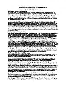
5: O-Rings Example Prediction of a binary response from features, or independent variables, did not start with data mining. It was my feeling in preparing this course that more long standing alternatives to data mining techniques should also be mentioned and to that end, I hoped to find an interesting real data example that uses logistic regression. Note that in the grammy example, the logistic function was used to generate the responses, but logistic regression was not used in the analysis. A real data example that serves well for this purpose is data on the space shuttle launches. The space shuttle Challenger was launched in air that was 31 degrees Fahrenheit, colder than previous launches. Tragically, an explosion just after liftoff destroyed the shuttle and killed all of the astronauts therein. Upon investigation, it was found that O-rings separating volatile elements of fuel were compromised because of the cold launch temperature. Prior to the disastrous launch of the Challenger, there had been 23 launches. Each launch involved 6 of these O-rings and evidence of problems with these, called erosion and blowby, were recorded for each ring. I constructed a dataset by recording a 0 or 1 for each of these 23x6 = 138 rings. A 0 was recorded if a ring had no evidence of damage and a 1 if either erosion or blowby were observed. Note that neither of these conditions is necessarily fatal – all 23 missions returned safely to earth. Nevertheless I will treat the observation of one of these conditions as a “failure” In the analysis that follows, I ignore the fact that the O-rings are not independent, this resulting from the fact that two rings on the same mission would be more alike in terms of stresses to which they were exposed, than two rings selected from different missions. Thus I simply run a logistic regression of this 0-1 response variable on the predictor variables or “features” as they are called in data mining. These features include the pre-launch temperature, the sequence 1-23 of the flight (as a check for possible time trend) and the results of a pre-launch pressure check. After reading in the data, this code is applied to produce a 3-D data plot with the vertical axis being the number of “failures” out of 6 rings for each of the 23 launches and the axes in the floor of the plot being temperature and launch number. PROC G3D DATA=shuttle; scatter launch*temp=failed / shape='prism' zmin=0 tilt=82 rotate=25; title "USA Space Shuttle Flights"; title2 "Failure = erosion or blowby";
7
SUGI 30
Data Mining and Predictive Modeling
Figure 4: Failures (out of 6 exposed)
It appears that failures are more common as we move toward the left (lower temperatures) and possibly as we move further out in the sequence of launches. Are either of these visual impressions backed up by statistics? In logistic regression, the thing that is being estimated is the probability of a failure (or success) p at a given setting of the independent variables, these being the “features” in data mining terminology. If modeling failures, we would expect an increasing probability as the temperature decreases and possibly some increase in probability over time at any given temperature. Logistic regressions can be fit using PROC LOGISTIC or PROC GENMOD and I took this opportunity to introduce both. *Estimate Logistic two ways*; PROC LOGISTIC DATA=shuttle; title3 "Logistic Regression"; model failed/atrisk = temp launch; output out=out1 predicted = p; PROC GENMOD DATA=shuttle; title3 "Logistic Regression"; model failed/atrisk = temp launch/dist=binomial; run; A partial result from the logistic fit is:
The LOGISTIC Procedure Analysis of Maximum Likelihood Estimates
Parameter DF Estimate Intercept 1 temp 1 launch 1
4.0577 -0.1109 0.0571
Wald ChiSq
Pr > ChiSq
1.7917 6.2122 1.0311
0.1807 0.0127 0.3099
Thus it appears that launch sequence is not significant but temperature is, with higher temperatures leading to lower probabilities of failure. The pre-launch pressure check was also insignificant when added to the regression (not shown). A grid of (temp, launch) values that included some points at the 31 degree Challenger temperature had been appended to the data so that extrapolation to that temperature could be done for this model. This also gave the opportunity to review the dangers of such extrapolation with the students.
8
SUGI 30
Data Mining and Predictive Modeling
**Plot prob(failure) vs. temp, launch # **; PROC G3D; plot launch*temp =p/ tilt = 82 rotate=25 zmin=0 zmax=1; where id = "grid"; label p = "Pr{O-ring failure}"; Comparing to the range of values in Figure 3, this is a rather large extrapolation. Keeping in mind these caveats, the graph of estimated failure probabilities is striking. The extrapolated probability of erosion or blowby on a given ring is about 87%, the height of the graph where it touches the vertical axis.
Figure 5: Estimated Probability
Another opportunity to review some basic concepts now presents itself. Recall that what we are calling “failure” is not really fatal, in that several shuttles have successfully returned to earth with one or two of the rings having experienced a problem. How about looking at the probability of, say, 4 or more failures out of the six rings on a mission? Since we have a value of p for each temperature and launch sequence value, we can compute the probability of 4 or more failures using the probability function for the binomial distribution with that p and n=6 trials. The probability becomes: 6 ⎛ ⎞ i 6! ⎟⎟ p (1 − p ) n −i Pr{6 or more}= ∑ ⎜⎜ i = 4 ⎝ j!(6 − j )! ⎠
and this can be computed using built-in SAS functions such as the binomial distribution function or the gamma function (Γ(i+1)=i!) as shown in this program segment: *Compute and plot Pr(4 or more failures) *; DATA NEXT; set out1; Prob_4=0; do i = 0 to 3; pi = gamma(7)/ (gamma(i+1)*gamma(7-i)); if _n_=1 then put pi; * check 6! /(i!)((6-i)!) *; pi = pi*(p**i)*((1-p)**(6-i));
9
SUGI 30
Data Mining and Predictive Modeling
prob_4 = prob_4 + pi; end; prob_4=1-prob_4; title3 "Pr{4 or more failures} vs. temperature & launch no."; PROC G3D; PLOT launch*temp =prob_4/ tilt = 82 rotate=25zmin=0 zmax=1; where id = "grid"; label prob_4 = "Pr{4 or more}";run;
Figure 6: Pr{4 or more out of 6}
Surprisingly, the probability that 4 or more will fail is higher than the probability that an individual will fail if the temperature is low enough, 97% when the temperature is 31. The slight rise as you move from the front to the back of the picture is a result of the inclusion of the insignificant sequence number in the model, its coefficient being a small positive number.
6: Extended Pens Example The University of California, Irvine keeps a collection of data mining test case data sets in their online UCI archive. An often used dataset consists of data from a handwriting recognition experiment. These data are used in some of SAS Institute’s data mining examples, often in the context of a classification tree. In this experiment, participants are asked to write digits on a pressure sensitive pad. Measurements consisting of 16 pen positions are taken for each written digit. The goal is to use these measurements to infer which digit is being written. Each observation is a vector of 16 numbers and a large collection of these vectors is available. One goal of this example is to encourage thinking about the data before mining it. Do we really need 16 numbers for each digit? Can we reduce the size of the vector before using EM? A classic method in this situation is principal components. Using PROC PRINCOMP to do this, here is a plot of the first two principal components using the digit number as a plot symbol. This would be followed by a decision tree or cluster analysis in EM using the principal components as features. This also affords an opportunity to briefly outline text mining which begins by a similar principal decomposition of word counts in documents. There you have rows in your data that represent documents and columns that represent words. The numbers in the data set are the counts of each word in each document so that there are as many columns as you have words in your “dictionary”. Principal components can be used to reduce the number of columns.
10
SUGI 30
Data Mining and Predictive Modeling
Figure 7: Digit Principal Components.
7: Conclusion Data mining has become a popular tool for analyzing large datasets. In the university environment, it seems important to give students some exposure to this popular topic. Because it is a university environment, this can include some ties to standard statistical methods and as a result, illustrate that the methods are actually quite similar to traditional statistics. In this paper I have presented some additions to the standard fare in a data mining course that I have used to accomplish this goal. ® : SAS and all other SAS Institute Inc. product or service names are registered trademarks or trademarks of SAS Institute Inc. in the USA and other countries. ® indicates USA registration. Other brand and product names are registered trademarks or trademarks of their respective companies.
References: Box, G. E. P. and Jenkins G. M. (1976) Time Series Analysis: Forecasting and Control. Holden-Day, San Francisco
Contact Information: David A. Dickey Department of Statistics, Box 8203 N.C. State University Raleigh, N.C. 27695-8203
[email protected]
11