1 Fractured Lattices, Integer Programming, and Diophantine Approximation? dedicated to Prof. Dr. Rainer Burkard (Graz) on the occasion of his 60th birthday G¨ unter Rote Institut f¨ ur Informatik, Freie Universit¨ at Berlin, Takustraße 9, D-14195 Berlin, Germany,
[email protected] Abstract. For a d-dimensional lattice Λ and a d-dimensional vector a we consider the sequence of point sets An := { ia + x | x ∈ Λ, 0 ≤ i < n } for increasing values of n. For the values of n when a new shortest nonzero vector appears in An+1 , the set An has a structure of a perturbed lattice, i. e., each point is in some small neighborhood of a (unique) lattice. We use this structure for a recursive approach to finding best approximations in fixed dimensions, with applications to integer programming. 2000 Mathematics Subject Classification: 11K60 Key words: best simultaneous Diophantine approximation, geometry of numbers.
1.1
Introduction
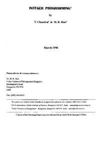
Integer Programming is of course closely connected to integer lattices and the geometry of numbers. Especially the algorithms in small dimensions which have theoretical performance guarantees are based on shortest vectors and good bases for integer lattices or at least approximations of them. The most notable instance is the polynomial-time algorithm of H. W. Lenstra [9] for integer programming in fixed dimensions. For integer programming in two dimensions, there are a number of different algorithms, the nicest (from a geometric viewpoint) being perhaps the algorithm of Kanamuru, Nishizeki and Asano [5]. All these algorithms, in one way or another, eventually boil down to some sort of continued fraction expansion or greatest common divisor computation. This is no surprise, since the greatest common divisor of two numbers a and b can be formulated as an integer programming problem min{ ax + by | ax + by ≥ 1, x, y ∈ Z } On the other hand, it has been shown that integer programming in two variables is no more difficult than greatest common divisor computation, at least as far as the “number-theoretic” complexity is concerned, the dependence on the size of the input numbers. (This does not account for the “combinatorial” (or “geometric”) complexity due to the fact that the problem may have a large number of constraints and the feasible region may be a complicated polytope, in higher dimensions.) Eisenbrand and Rote [3] introduced a novel parametric approach to integer programming in two variables. They reduced it to the following key problem. The Parametric Shortest Vector Problem. Let a two-dimensional lattice Λ and a parameter ε be given. Find the smallest factor l such that scaling the y-coordinate by l produces a lattice whose shortest vector (in the max-norm) has length ε. Of course, the problem has no solution if the x-axis contains a vector shorter than ε. Otherwise, it is easy to see that l can be calculated by solving the following problem, see Figure 1.1. ?
submitted for publication to Monatshefte f¨ ur Mathematik, December 2002
2
G¨ unter Rote
2ε
a ˜ 0 Fig. 1.1. The Best Approximation Problem for a two-dimensional lattice Λ
Let a two-dimensional lattice Λ be given. Find the lowest lattice point of the upper half-plane inside a given vertical strip of width 2ε that is centered at the origin. In [3], the problem is solved by direct application of an algorithm of Sch¨ onhage [12] for best rational approximation. This paper arose from an effort to extend this approach to higher dimensions. We will discuss the higher-dimensional version of the problem and derive some structural properties. We will also give an algorithm, although its running time is not competitive with the best other algorithms [4]. We formulate the higher-dimensional problem a follows. The Best Approximation Problem. Let a (d+1)-dimensional lattice Λ˜ ⊂ Rd+1 and an error tolerance ε be given. Find the lattice point with smallest positive xd+1 -coordinate that lies within a distance ε of the xd+1 -axis. The distance from the xd+1 -axis can be measured by some arbitrary norm, but we will stick mostly to the usual Euclidean norm This problem is just a reformulation of the classical Diophantine approximation problem: We want to approximate a set of d numbers α1 , . . . , αd by rational numbers x1 /Q, . . . , xd /Q with a common denominator Q. If we multiply the approximating numbers by Q, we see that this problem amounts to finding an integer vector (x1 , . . . , xd , Q) ∈ Zd that lies close to the line generated by the vector (α1 , . . . , αd , 1). We just have to transform this line into the xd+1 -axis leaving the other axes fixed, and measure the “distance” from the axis appropriately, namely in the max-norm, to get our formulation of the Best Approximation Problem. We can split the lattice into layers as follows, see Figure 1.1. We assume that the sublattice Λ := { x ∈ Λ˜ | xd+1 = 0 } is d-dimensional. This is no loss of generality if ˜ Λ˜ consist of rational points. Let a ˜ be a vector which, together with Λ, generates Λ. ˜ Then Λ consists of horizontal level Λ + i˜ a, for i ∈ Z. We write a ˜ = (a, ad+1 ) with a ∈ Rd , and assume ad+1 > 0. Then the Best Approximation Problem amounts to the following problem: Find the lowest level Λ + i˜ a (i ≥ 1) which contains a point within ε of the xd+1 -axis. Since the xd+1 -coordinate is irrelevant for measuring the distance from the xd+1 axis, we obtain the following equivalent formulation in Rd . Find the smallest i ≥ 1 such that Λ + ia contains a point within ε of the origin.
1
Fractured Lattices, Integer Programming, and Diophantine Approximation
3
We denote the union of the first n − 1 layers by An := { ia + x | x ∈ Λ, 0 ≤ i < n } Hence we arrive at the following problem formulation, which is the one we will use in the paper. Find the smallest n ≥ 1 such that An contains a nonzero point of length less than ε. (This formulation is not completely equivalent, because Λ might already contain a point of length at most ε, or the desired short point at level i might be the zero vector. These cases have to be checked separately.) 1.1.1
Related Work
The Shortest Vector Problem. We solve the Best Approximation Problem in a sequence of rounds, repeatedly increasing n and looking for a vector in An that is shorter than the previously found shortest vector. Thus, during the course of the ˜ Either this vector lies algorithm, we will also find the shortest non-zero vector of Λ: in Λ, or it lies in one of the other levels Λ + ai. In that level, it must clearly be the closest point to the xd+1 -axis, and there can be no point which is as close to the xd+1 -axis in any of the levels below the i-th level. The process can be stopped as soon as the distance from the hyperplane of the current level to the origin is larger than the shortest vector found so far. The shortest vector problem, and the related problem of finding a good lattice basis, are important for other areas like algebraic number theory or the analysis of pseudo-random number generators. The best general algorithm in arbitrary dimension d is the algorithm of Lov´ asz [8], which computes in polynomial time a d−1 vector which is at most 2 2 times longer than the shortest vector. This algorithm starts with some lattice basis, and repeatedly performs lattice reductions in the two-dimensional lattice spanned by pairs of basis vectors. Schnorr [11] has extended this algorithm so that it looks at k-tuples of vectors and reduces the corresponding k-dimensional sublattices. The algorithm runs in a polynomial number of iterations for fixed k and achieves an approximation factor d of (6k 2 ) 2k . Thus, any progress in lattice reduction algorithms for fixed dimension k has an impact on algorithms for arbitrary dimensions. In fixed dimension, the problems of best approximation, of computing a short lattice vector, of computing a “good” lattice basis or even of enumerating all reduced lattice basis (in a very weak sense) are all computationally equivalent, see [4, Section 6]. There running time is within a constant factor of each other. Continued Fractions. Multi-dimensional continued fraction are also related to best approximations, see [1] for an overview. However, in this area, it is customary to define some procedure (like the classical Jacobi-Perron algorithm), and then try to analyze its behavior. In contrast to this, the algorithm that we describe is found by specifying its behavior clearly in geometric terms. Quasiperiodic tilings. From the above description, the set An arises as a section of the (d + 1)-dimensional lattice Λ˜ between two parallel hyperplanes, projected to a d-dimensional space. Such projections of slices of higher-dimensional lattices are also used to generate quasiperiodic point sets, tilings, and quasicrystals by the cut-and-project method, see [13,10].
4
G¨ unter Rote
1.1.2
Overview.
In Section 1.2 we will discuss how the set An evolves as n increases. In particular, we will be interested in the points when a new shortest nonzero vector appears, because this is a candidate for the solution of the Best Approximation Problem. In particular, we will define the structure of a fractured lattice. In Section 1.3 we will use the properties that we have found for defining an algorithm that solves the Best Approximation Problem recursively by reducing it to lower-dimensional problems.
1.2
The Structure of An
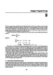
In the following, the concepts will be illustrated with examples in the plane, but unless otherwise stated, they hold in any dimension. We will use the language that is appropriate for the planar case; for example, we will speak of disks when balls would be the proper term for higher dimensions.) Figure 1.2 shows the set A27 for the two-dimensional lattice Λ generated by the vectors (1, 0) and (0, 1) and for the vector a indicated in the figure. Since the point set is periodic with the period of Λ, we only show the range [−0.5, 0.5]2 around the origin. The last point added is point 26, and it is the nearest neighbor of the origin among the points added so far. 13
20
0.4
1
8
15
22
3
0.2
a
17
10 24
5
12
0
19
26 0
7
14
21
−0.2
2
9 16
−0.4
23
4
11
18
25
−0.4
−0.2
0
6
0.2
0.4
Fig. 1.2. The point set A27 . The point labeled i is ia mod Λ
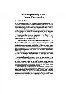
We will regard An as a set of n vectors 0, a, 2a, . . . , (n − 1)a modulo Λ. The vector x mod Λ will denote the congruence class x + Λ and we can perform vector additions and multiplications by integer scalars with these congruence classes as with usual vectors. We denote congruence by x ≡ y (mod Λ), and we will usually omit (modΛ) because the lattice Λ is clear from the context. It is visually apparent that the point set in Figure 1.2 has a somewhat latticelike regular structure. This structure is shown in Figure 1.3. We call this a fractured lattice. A fractured lattice is determined by a fracture vector f , and instead of d basis vectors, it is characterized by d pairs of “basis vectors” {u1 , u1 +f }, . . . , {ud, u1 +f }.
1
Fractured Lattices, Integer Programming, and Diophantine Approximation
13
20
0.4
1
8 u2 +f
0.2
15
22
3
10
17 u1 +f
u2
12
0
26 7
f
5
24 19
0
u1
14
21
−0.2
2
9
16
23
4
−0.4
11
18
25
−0.4
5
−0.2
6
0
0.2
0.4
Fig. 1.3. The point set A26 and the fractured lattice
Lemma 1. Assume that the vectors 0, a, 2a, . . . , (n − 1)a are distinct modulo Λ. Then the set An has the structure of a fractured lattice, in the following sense: For every x and for every i = 1, . . . , d, the following holds. • x + ui ∈ An or x + (ui + f ) ∈ An , but not both. • x − ui ∈ An or x − (ui + f ) ∈ An , but not both. We call these 2d points the neighbors of x. Moreover, An is connected by this neighborhood relation. For f = 0, this definition coincides with the usual concept of a lattice. Proof. Let z1 , . . . , zd be positive integers less than n with gcd(z1 , . . . , zd , n) = 1. Then the vectors ui ≡ zi a and f ≡ −na will form the fractured lattice. To see this, let x ≡ ja ∈ An , for some 0 ≤ j < n. If j + zi < n, then (j + zi )a ≡ x + ui ∈ An . Otherwise, 0 ≤ j + zi − n ≤ n, and (j + zi − n)a = x + (ui + f ) ∈ An . Both possibilities cannot hold simultaneously. Otherwise we would have two vectors in An whose difference is f : ja + f ≡ j 0 a, with 0 ≤ j, j 0 < n. If j < j 0 it follows that (n − 1)a ≡ (j 0 − j − 1)a, contrary to the assumption that all points in An are distinct. If j > j 0 , then 0 ≡ (j 0 − j + n)a ∈ An , again a contradiction. The case where we want to subtract ui or ui + f from x works similarly. To show that any two vectors ja, j 0 a ∈ An are connected, note that the equation j + k1 z1 + k2 z2 + · · · kd zd ≡ j 0
(mod n)
has an integer solution (k1 , . . . , kd ) by assumption. Thus we can transform ja into j 0 a by repeatedly adding or subtracting ui of ui + f (as appropriate), the given number of times |ki |. The result is a vector j 00 a ∈ An with 0 ≤ j 00 < n and j 00 ≡ j 0 (mod n), and hence it must be j 0 a. t u This proof is quite trivial. Note that we did not exclude the possibility z1 = z2 = · · · = zd , and hence the basis vectors ui need not even be distinct. However, the lemma might not give what is suggested by the picture in Figure 1.3. The fracture vector f ≡ −na mod Λ might be very long compared to the “basis vectors” ui , and
6
G¨ unter Rote
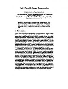
hence the structure is not really visible. However, when na is a best approximation, then we may choose some “good” basis vectors and the structure becomes apparent. When na is a best approximation, then the set An is also a perturbed lattice, in the sense that the points can be moved slightly so that they form a real lattice. Figure 1.4 shows this lattice for the point set of Figure 1.3. 13
20
0.4
1
8
15
22 3
0.2
10
17
24
5
12
0
19
0
26 7
2
14 21
−0.2
9
16
−0.4
24
23 4
11 25
18 6
−0.4
−0.2
0
0.2
0.4
Fig. 1.4. The point set A26 is approximated by the lattice Λˆ shifted by f 0 , which is indicated by the grid of lines. The little disks indicate the largest perturbation error ε
This lattice has been introduced by Larcher [7], and the following theorem is essentially given in [2] (apart from the statement about the bijection). First we state an easy observation. Lemma 2. The length of the shortest vector of An is a lower bound for the distance between two points of An Proof. The distance between two points ja and j 0 a is kja − j 0 ak = |j − j 0 |a, which t u is the length of some vector of An . Let n0 = 1 < n1 < n2 < · · · < nt−1 be the sequence of indices n when An+1 contains a non-zero vector which is shorter than the previous shortest vector (a best approximating vector). We define the last index nt as the first level Λ + ia which contains the zero vector; the set An will remain stable for n ≥ nt . This last index must exist when the data are rational. If a or Λ are not rational, then the sequence n0 , n1 , . . . may be infinite. Theorem 1. For n = n1 , n2 , . . ., let f ≡ na be the shortest non-zero vector in An+1 . (For n = nt , let f = 0.) Then there is a d-dimensional lattice Λˆ and a bijection π between An and Λˆ such that kˆ x + f 0 − xk ≤ ε, ˆ = π(x), with for all x ∈ An and x f0 = f ·
n−1 and ε = kf k. 2n
(1.1)
1
Fractured Lattices, Integer Programming, and Diophantine Approximation
7
Moreover, the given value ε is the smallest value for which such a lattice exists, and the lattice Λˆ is the unique lattice that fulfills (1.1) for any ε < kf k. Proof. Λˆ is generated by Λ and the vector a ˆ := a − f /n. Since nˆ a = na − f ≡ 0, it is indeed a discrete lattice, with at most n congruence classes modulo Λ. The a, and we get x − x ˆ ≡ ja − jˆ a = jf /n, mapping π : An → Λˆ is given by π(ja) := jˆ for j = 0, 1, . . . , n − 1. To balance this error between the two extreme cases j = 0 and j = n − 1, we shift x ˆ by f 0 = 12 · (n − 1)f /n: xˆ + f − x ≡ ( n−1 2 − j)f /n, for some 0 ≤ j ≤ n − 1, and the length of this vector is at most ε. (This is true for any norm.) The mapping π must be injective, since two points ja and j 0 a that are mapped to the same point are within distance ε of a common point, and hence kja − j 0 ak ≤ 2ε < kf k. By Lemma 2, this contradicts the assumption that f is the shortest vector. t u
65 39 13
20 0.4
8 60 34
0.2
10 62 36
17 69 43
33 7
23 75 49
4 56 30 25 77 51
−0.4
2 54 28
9 61 35
11 −0.4
59 14 66 40
21 73 47 16 68 42
−0.2
24
19 71 45
26 0 78 52
0
76 50
5 57 31
12 64 38
−0.2
15 67 41
22 74 48
3 55 29
72 46
1 53 27
18 70 44 0
63 37 58 32 6 0.2 0.4
Fig. 1.5. The point set A79 . Each point x = 0, a, 2a, . . . , 25a has received two neighbors x + f and x + 2f , and point 0 has just received its third neighbor
1.3
Inductive construction of good fractured lattice bases
We will now see how a good “basis” for a fractured lattice or for Λˆ can help us to understand the further evolution of the set An . Consider the situation in Figure 1.2. Point 0 has just received a new nearest neighbor f ≡ na. The next point (n + 1)a = 28a will be a neighbor of a, and then the points 2a, 3a, and so on will get neighbors, by the relation (n + j)a ≡ ja + f , see Figure 1.5. Once all points 0, . . . , (n − 1)a
8
G¨ unter Rote
0.4
3
29
55
0.2 95 147 121
43
38
12
83 135 109
64
−0.2
78 130 104
125 99
73
42
16
68
−0.4
7
11
47
−0.4
51
21
25
56
26
52
62
36
10
5
128 102
30
−0.2
81 133 107 24 76 50 116 142
19
97 149 123
71
66
40
14
85 137 111
9
80 132 106
61
35
4
75 127 101
96 148 122
138 15
41
45
92 144 118
87 139 113
82 134 108
103 77
67
0
0 33
93 145 119
31
57
72
124 98
1
27
88 140 114
17
69
90
22
48
74 126 100
46
53
79 131 105
8
34
60
112 86
136 110
13
39
65
91 143 117
20
70
44
18
49
0.2
58
2
94 146 120
89 141 115 84
0
23
28
54
59
63
32 6
37
129
0.4
Fig. 1.6. The point set A150
have received their neighbors, point 0 will receive a second-degree neighbor 52a, which is a neighbor of 26a, and similarly for the other points. Then there will be third-degree neighbors, and so on. Although this structure has some regularity, it does not approximate a lattice. Only when a new nearest neighbor appears (this is 149a in Figure 1.6), another approximate lattice structure emerges. Now let us imagine that we stand at the origin and wait until a point arrives which has a smaller length than f = na, the shortest vector so far. A typical situation is shown in Figure 1.7. All points of An start “shooting” in the direction of f , by successively generating neighbors at distance f, 2f, 3f, . . .. We are interested in the first point which hits the small disc of radius kf k around the origin. The set An can be divided into (d − 1)-dimensional layers according to the fractured lattice structure. If the layers are sufficiently well “separated”, as in Figure 1.7, we can ask for the first layer whose shooting ray in direction f hits the small disk. A schematic picture is shown in Figure 1.8. The shooting direction is vertical downward, we have arranged each layer on a horizontal line and placed the layers on successive levels. The origin with the target disc lies on the horizontal ground line. Now, the points in this drawing form a lattice: The difference vectors between neighbors are of the form ±ui or ±(ui + f ), by the fractured lattice structure. The irregularity introduced by the fracture vector f is projected away in this process, since we are only interested in rays parallel to f through the points. This observation is the main geometric insight on which our algorithm is based. The situation in Figure 1.8 is now almost the same as the picture of the Best Approximation Problem in two dimensions shown in Figure 1.1. In other words, the
1
Fractured Lattices, Integer Programming, and Diophantine Approximation
9
j ui + f ui
j+n j + 2n j + 3n 0 f n 2n 3n
Fig. 1.7. The points of An are arranged in successive layers and shoot in direction f
problem that we face is of the same kind as the original problem, but one dimension lower.
0
Fig. 1.8. A schematic picture of the shooting process
There are some differences, however. If we ask which ray in direction f is the first one that hits the disk, we can replace the disk by its intersection with the ground line (the thick segment in Figure 1.8). In higher dimensions, this target is not a segment but a (d − 1)-dimensional ball. Thus we would get exactly the Best Approximation Problem in one dimension lower. However, the neighbors are generated for the points of An in discrete steps and don’t fill a ray densely. It may happen that some ray in direction f passes through the disc but none of the points fall in the disk, see Figure 1.9a. We call this a phase error because it depends on the locations of the equidistantly placed points on the ray.
10
G¨ unter Rote
j2 j1 j1
j2
0 f
0
j1 +2n j2 +3n
j2 +n
f
j1 +3n (a)
(b)
Fig. 1.9. (a) A phase error. The first point whose ray in direction f hits the disk is j1 , but the points j1 + n, j1 + 2n, . . . miss the disk. The first point that really falls in the disk comes later from j2 . (b) A sequence error. The point j1 lies on a lower layer than j2 but the sequence of points starting at j2 hits the disk first
There is another source of error, a sequence error. It may happen that the levels are not so clearly separated, and a point on a later layer hits the disk first, see Figure 1.9b. This phenomenon may occur when the layers form a small angle with the shooting direction. It may also happen that sequences of points emanating from two points on the same layer of An hit the disk in the wrong order. To deal with these problems, we sometimes have to continue the procedure even after finding the “first” ray that hits the horizontal segment, in order to build a safety margin. The Repeated Best Approximation Problem is like the Best Approximation Problem defined in Section 1.1, but after the lowest lattice point within a distance ε of the xd+1 -axis is found, we may also ask for the second-lowest, the third-lowest, and so on (up to some constant bound that depends only on the dimension). The Repeated Best Approximation Problem Enumerate the points ia + x, i > 0, x ∈ Λ, with kia + xk < ε in order of increasing i. In our application of this problem, we will have ε ≤ min{ kxk | x ∈ Λ, x 6= 0 }. Then the number of points with the same value of i is bounded by a constant that depends only on the dimension, by Lemma 2. Lemma 3. In each dimension, there is some constant bound Cd1 on the number of times that a phase error can occur. Proof. This is a volume packing argument. For each ray that hits the vertical projection of the disk, there must be a point generated that falls into the bounding box vertical cylinder circumscribed about the disk. (This appears as a circumscribed square in Figure 1.9a). By Lemma 2, these points must have a minimum distance of kf k as long as no point lies within the disk. The box can only contain a constant
1
Fractured Lattices, Integer Programming, and Diophantine Approximation
11
Input: A lattice basis u1 , . . . , ud , a vector a, and a threshold ε. Output: A sequence of points x = z1 u1 + · · · + zd ud + ia for the Repeated Best Approximation Problem. Initialization: Set f := a; Main loop: Select one vector of the current basis. (For convenience, let us assume it is ud .) Let u01 , . . . , u0d denote the projection of u1 , . . . , ud onto the hyperplane perpendicular to f . Solve the (d − 1)-dimensional Repeated Best Approximation Problem for u01 , . . . , u0d−1 , a0 := u0d and ε0 := kf k. This will enumerate the successive points y = z1 u01 + · · · + zd u0d with kyk < kf k in order of increasing zd > 0. For each point y, find all i ∈ Z such that x = z1 u1 + · · · + zd ud + if satisfies kxk < kf k. If enough points have been generated to be sure that the point x with minimum i has been found, then let f be this vector. If kf k > ε, update the basis u1 , . . . , ud and repeat the loop. Output the generated points x with kxk < ε in order of increasing i. Fig. 1.10. The recursive algorithm for the Repeated Best Approximation Problem
number of points with minimum separation kf k. (This argument can be adapted to other metrics. In the (d − 1)-dimensional problem one works with a projection of a d-dimensional unit ball, or with a suitable enclosing body that is easier to handle.) t u The recursive algorithm is schematically shown in Figure 1.10. To take care of the sequence error, we have to relate the order of the points x = z1 u1 + · · · zd ud + if with kxk < kf k according to zd , in which the points are generated, to the desired order according to i. We use the following lemma. Lemma 4. Let x = z1 u1 + · · · + zd ud + if and x0 = z10 u1 + · · · + zd0 ud + i0 f be two points with kxk ≤ kf k and kx0 k ≤ kf k, and let zd0 ≥ zd . Then i0 ≥ i − C for C = 3ku∗dk · kf k, where u∗1 , . . . , u∗d is a basis of the dual lattice. Proof. Let y = z1 u1 + · · · + zd ud and y 0 = z10 u1 + · · · + zd0 ud be the corresponding points of the lattice. Then we have zd = hy, u∗d i and zd0 = hy 0 , u∗d i, and if − i0 f = (x − y) − (x0 − y 0 ) = (x − x0 ) − (y − y 0 ). By taking the inner product with u∗d , we obtain i − i0 ≤ zd − zd0 + kx − x0 k · ku∗d k. We have kx − x0 k ≤ 2kf k, and we have to add kf k because of the error bound between the point set An and the lattice (Theorem 1). t u Since f is shorter than the shortest vector of the lattice, the product ku∗d k · kf k is bounded by a constant which depends only on the dimension. It follows that, in fixed dimension, the algorithm has to wait only a constant number of rounds after the first point x = z1 u1 +· · ·+zd ud +if with kxk ≤ kf k (the point x with smallest zd ) has been found before it can start to output x. Thus the
12
G¨ unter Rote
algorithm has to accommodate a buffer for a limited number of points. In addition, for some points y which are generated, there may be no integer value i such that kz1 u1 +· · ·+zdud +if k < kf k. The occurrence of these phase errors is also bounded, by Lemma 3. Thus we can conclude: Lemma 5. In one iteration of the main loop, there is a constant number of calls to the (d − 1)-dimensional Repeated Best Approximation Problem. t u The number of iterations is equal to the number of best approximations, which is known to be logarithmic in the size of the input numbers [6]. Theorem 2. For fixed d, the algorithm reduces the d-dimensional Repeated Best Approximation Problem with input numbers of s bits to O(s) instances of the (d−1)dimensional Repeated Best Approximation Problem. Therefore, the d-dimensional Repeated Best Approximation Problem is solved in t u O(sd ) steps.
1.4
Conclusion
The algorithm that we have given is not competitive with the fastest theoretical algorithm in fixed dimension [4], which reduced the problem to only O(logd s) greatest common divisor computations. However, the simple and in some sense, canonical structure may be the key to an algorithm in the style of Sch¨ onhage’s algorithm for the two-dimensional problem [12], which solves the problem only approximately for the leading half of the bits of the numbers, and then extends this solution to the full numbers (the “half-GCD” approach). A canonical procedure like the continued fraction expansion (the Euclidean algorithm) seems crucial for the success of this approach. We have not analyzed the constants in the algorithm. They depend on relations between a lattice and its dual lattice and on packing arguments, for which precise estimates are hard to obtain, even in three dimensions.
References 1. A. J. Brentjes, Multi-dimensional continued fraction algorithms, Mathematical Centre Tracts, vol. 145, Mathematisch Centrum, Amsterdam, 1981. 2. Nicolas Chevallier, Meilleures approximations diophantiennes d’un ´ el´ement du tore T2 et g´eom´etrie de la suite des multiples de cet ´el´ement, Acta Arith. 78 (1996), 19–35. 3. Friedrich Eisenbrand and G¨ unter Rote, Fast 2-variable integer programming, IPCO 2001—Proceedings of the 8th Conference on Integer Programming and Combinatorial Optimization, Utrecht (K. Aardal and B. Gerards, eds.), Lecture Notes in Computer Science, vol. 2081, Springer-Verlag, 2001, pp. 78–89. 4. , Fast reduction of ternary quadratic forms, Cryptography and Lattices — International Conference, CaLC 2001 (Joseph H. Silverman, ed.), Lecture Notes in Computer Science, vol. 2146, Springer-Verlag, 2001, pp. 32–44. 5. Naoyoshi Kanamuru, Takao Nishizeki, and Tetsuo Asano, Efficient enumeration of grid points in a convex polygon and its application to integer programming, Internat. J. Comput. Geom. Appl. 4 (1994), 69–85. 6. Jeff C. Lagarias, Best simultaneous diophantine approximations. I: Growth rates of best approximation denominators, Trans. Am. Math. Soc. 272 (1982), 545–554. 7. G. Larcher, On the distribution of s-dimensional Kronecker sequences, Acta Arithmetica 51 (1988), 335–347. 8. A. K. Lenstra, H. W. Lenstra, Jr., and L. Lov´asz, Factoring polynomials with rational coefficients, Math. Ann. 261 (1982), 514–534. 9. H. W. Lenstra, Integer programming with a fixed number of variables, Math. Oper. Res. 8 (1983), 538–548.
1
Fractured Lattices, Integer Programming, and Diophantine Approximation
13
10. Yves Meyer, Quasicrystals, diophantine approximation and algebraic numbers, Beyond Quasicrystals. Papers of the winter school, Les Houches, France, March 7–18, 1994. (Fran¸coise Axel and D. Gratias, eds.), Springer, Berlin, 1995, pp. 3–16. 11. C. P. Schnorr, A hierarchy of polynomial time lattice basis reduction algorithms, Theoret. Comput. Sci. 53 (1987), 201–224. 12. Arnold Sch¨ onhage, Schnelle Berechnung von Kettenbruchentwicklungen, Acta Informatica 1 (1971), 139–144. 13. Marjorie Senechal, Quasicrystals and geometry, Cambridge University Press, 1996.