Department of Civil & Environmental Engineering, Imperial College, London ... consolidation problems and was implemented in the FE program ICFEP (Imperial.
Stability Investigation of the Generalised-α Time Integration Method for Dynamic Coupled Consolidation Analysis Bo Han, Lidija Zdravković, Stavroula Kontoe Department of Civil & Environmental Engineering, Imperial College, London SW7 2AZ, United Kingdom
Abstract. In this paper, the stability of the Generalised-α time integration method (the CH method) for a fully coupled solid-pore fluid formulation is analytically investigated for the first time and the corresponding theoretical stability conditions are proposed based on a rigorous mathematical derivation process. The proposed stability conditions simplify to the existing ones of the CH method for the one–phase formulation when the solid-fluid coupling is ignored. Furthermore, by degrading the CH method to the Newmark method, the stability conditions are in agreement with the ones proposed in previous stability investigations on coupled formulation for the Newmark method. The analytically derived stability conditions are validated with finite element (FE) analyses considering a range of loading conditions and for various soil permeability values, showing that the numerical results are in agreement with the theoretical investigation. Then, the stability characteristics of the CH method are explored beyond the limits of the theoretical investigation, assuming elasto-plastic soil behaviour which is prescribed with a bounding surface plasticity constitutive model. Since the CH method is a generalisation of a number of other time integration methods, the derived stability conditions are relevant for most of the commonly utilised time integration methods for the two-phase coupled formulation. Key Words: stability condition, CH method, dynamic analysis, finite element method, coupled formulation
1. Introduction In dynamic FE analysis, time integration schemes have been widely and successfully used to solve the second order governing equation of motion, as they can incorporate both material and geometric nonlinearities. Since 1950s, various time integration methods have been proposed, such as the Newmark (Newmark, 1959), HHT (Hilber et al., 1977), WBZ (Wood at al., 1981) and Generalised-α methods (CH method) of Chung 1
and Hulbert (1993), which have been widely implemented into FE programs and successfully utilised to solve numerically the equation of motion for one-phase materials. The CH method satisfies the main requirements for an efficient time marching algorithm, which include unconditional stability for linear problems, second order accuracy and controllable numerical dissipation in the high frequency range (Hilber and Hughes, 1978). The role of numerical damping is to eliminate spurious high-frequency oscillations that are introduced into the solution due to poor spatial representation of the high-frequency modes. Depending on the range of soil permeability and dynamic loading duration, it is often necessary to employ coupled consolidation analysis to accurately model the two-phase soil behaviour. Dynamic analyses are further complicated by the presence of the inertia forces of the different phases (i.e. solid skeleton and pore water) and the coupling between them. Hence, the formulation of the CH method was extended by Kontoe (2006) and Kontoe et al. (2008b) to enable the solution of dynamic coupled consolidation problems and was implemented in the FE program ICFEP (Imperial College Finite Element Program) (Potts and Zdravković, 1999). Over the last decade the CH method has been used for the dynamic analysis of geotechnical problems involving both one-phase (e.g. Kontoe et al. 2008b, 2012; Nazem et al. 2009) and two-phase formulations (Sabetamal et al. 2014). The key feature of unconditional stability of this method has been comprehensively investigated by previous studies, both analytically and numerically, but only for the one-phase formulation (Chung and Hulbert, 1993). The two-phase coupled FE formulation requires an additional equation (the dynamic consolidation equation) and an additional unknown (pore water pressure). Aiming to solve two dynamic coupled equations (i.e. the equation of motion and the consolidation equation), the time integration method is applied to both equations. This not only increases the complexity of the implementation, but it also changes the numerical features of the time integration method. Therefore, the numerical stability of the CH method needs to be investigated rigorously for two-phase coupled problems. In this paper, the stability of the CH method for the coupled formulation is systematically investigated for the first time and the corresponding theoretical stability conditions are derived. The analytically derived stability conditions are validated by FE analyses and the stability characteristics of the CH method are further investigated considering a range of loading conditions, model geometries and constitutive models. 2
Furthermore, since the CH method is a generalisation of the Newmark, HHT and WBZ methods, the stability investigation of the CH method for the two-phase coupled formulation is relevant for most of the commonly utilised time integration methods.
2. The CH method for the coupled dynamic formulation The principle of the CH method is that the acceleration, velocity, displacement and pore fluid pressure terms are evaluated at different instances within a time step, Δt, controlled by integration parameters m and f (shown in Equation (1)). The variations of velocity and displacement within a time step for the CH method are approximated by Newmark’s equations, governed by the integration parameters and
(shown in Equation (2)). Kontoe (2006) and Kontoe et al. (2008b) showed that the final dynamic FE coupled consolidation formulation for the CH method can be described by Equation (3) (sign convention: tension positive), where five integration parameters, m , f , , and , are involved. It should be noted that is the integration parameter of a time marching scheme which is employed in ICFEP to solve the integrals of the consolidation equation, as shown in Equation (4) (Potts and Zdravković, 1999). In particular, as illustrated in Figure 1, the pore fluid integral on the left hand side of Equation (4) is represented by the grey area, which can be approximated by the hatched area through adopting the time marching scheme. Based on the principle of this time marching scheme, the values should be bounded between 0 and 1. Furthermore, according to Booker and Small (1975), in order to ensure the stability of the employed time marching scheme for static consolidation problems,
should be equal or larger than 0.5. dtk 1m 1 m dtk 1 m dtk dtk 1 f 1 f dtk 1 f dtk dtk 1 f 1 f dtk 1 f dtk ptk 1 f 1 f ptk 1 f ptk tk 1 m 1 m tk 1 m tk tk 1 1 f tk 1 f tk f d
t
d
dt 1 t dt 2 k
1 1 1 d d d tk dt t 2 t 2 k
(1)
k
(2)
3
1 1 f m M C 1 f t t 2 1 m G 1 L T f t
K
d R p F 1 f t Φ S
1 L f
(3)
tk t
pdt p p t p 1 p t tk
tk 1
tk
(4)
tk
Figure 1: Approximation of pore water pressure integral (after Potts and Zdravković (1999))
The coupled dynamic formulation (Equation (3)) was derived based on the dynamic equilibrium of the solid-fluid mixture, the continuity equation of the pore fluid flow and the generalised Darcy’s law. In the above equations, M , C , K , L , Φ and
S are
the global mass, damping, stiffness, coupling, permeability and water
compressibility matrices respectively, and 𝑑̈ , 𝑑̇ , 𝑑 and 𝑝 represent the nodal acceleration, velocity, displacement and pore fluid pressure variables respectively. It should be noted that the matrix G in Equation (3) represents the impact of the inertia of the solid on the pore fluid pressure. It has been though suggested that the influence of the matrix G on the dynamic response is insignificant for the frequency range within which the “u-p” formulation is valid (Chan, 1988). Therefore, the matrix G is not taken into account in the dynamic coupled formulation for the work presented herein. Furthermore, the matrices and the right hand side terms of Equation (3) are detailed in the Appendix.
3. Stability investigation of the CH method for the coupled formulation Since the stability of a time integration method is a key numerical feature, 4
researchers have extensively investigated the stability of the widely used time integration methods, i.e. Newmark (1959), Hilber et al. (1977), Wood et al. (1981) and Chan (1988). As an increasingly widely employed time integration method, the stability of the CH method was also studied by Chung and Hulbert (1993), but only for the one-phase formulation. In this part, the stability of the CH method for a fully coupled dynamic consolidation formulation is systematically investigated and the unconditional stability conditions are proposed. The stability investigation presented in this section follows a four-step procedure. First, the accumulated scalar form of the coupled dynamic formulation is derived based on the FE formulation presented in the previous section. Second, the expressions of the Newmark method for the variation of velocity and displacement within a time step are utilised in the accumulated scalar form of the coupled dynamic formulation. Third, the approximations of the CH method for various variables are employed in the dynamic formulation. Last, the stability of the CH method is investigated based on the derived formulation which includes only two variables: the incremental acceleration and pore fluid pressure. According to Bathe (1996), a time integration method is considered stable when it produces a numerical solution which remains always bounded. The fundamental assumption of the time integration method is that the acceleration, velocity and displacement at a specific increment can be expressed as a function of these variables at previous increments, as shown in Equation (5), where A is the amplification matrix controlling the stability, accuracy and other numerical features of the considered time integration method. Based on the definition of numerical stability, for a time integration method to be stable, the matrix A should be bounded. Therefore, the modulus of the eigenvalues of matrix A should be less or equal to one, expressed by Equation (6), where ρ is the spectral radius of the matrix
A
and 1 , 2 and 3 are the
eigenvalues of the matrix A . The Routh-Hurwitz condition, which has been widely employed in the stability analysis of various time integration methods (Wood, 1990), is adopted in this study. In particular, it is suggested by Routh (1877) and Hurwitz (1895) that, if λ is substituted by a function of a complex number z (as shown in Equation (7)), the condition of 1 can be converted to the condition of Rez 0 , indicating that the real part of z should be less or equal to zero in order to satisfy the stability condition.
5
Furthermore, for a general polynomial of the form shown in Equation (8) to satisfy the condition of Rez 0 , the conditions of Equations (9) and (10) should be satisfied. Therefore, the stability condition of 1 is finally converted to the conditions given by Equations (9) and (10), which will be used for the following stability analysis of the CH method.
dtk 1 dtk d tk 1 Adtk d d tk 1 tk
(5)
A max1 , 2 , 3 1
(6)
1 z 1 z
(7)
a0 z n a1 z n1 a2 z n2 ....an 0
(8)
a0 0 and ai 0
for i 0
a1 a2 a3 a0 a32 a4 a12 0
(9) (10)
3.1 Scalar form of the coupled dynamic FE formulation In order to analyse the stability of the CH method, it is simpler to use the accumulated scalar form of the coupled dynamic formulation. For the equation of motion, the accumulated scalar form after utilising the CH method is shown in Equations (11) and (12), where m, c, k and l are the scalar forms of the matrices M ,
C , K
and L respectively. Furthermore, the scalar form of the consolidation
equation is shown in Equation (13), where φ and s are the scalar forms of the matrices
Φ
and S . m dtk 1m c dtk 1 f k dtk 1 f l ptk1 f 0 dtk 1m 1 d m tk 1 dtk 1 f 1 f dtk 1 dtk 1 f 1 f dtk 1 p 1 p f tk 1 tk 1 f
1 f pk p 1 f s
m d tk f d tk f d tk f ptk
p d 1 f l T 0 t t
(11)
(12)
(13) 6
3.2 Application of the expressions of the Newmark method Based on the fundamental principle of the time integration method, the acceleration, velocity and displacement at time increment t k 1 can be expressed as a function of their historic values, as shown in Equation (14) after employing the Routh-Hurwitz condition. dtk 1 dtk d tk 1 1 z dtk d tk 1 1 z d tk pt pt k 1 k
(14)
The left hand side of Equation (14) is rewritten in incremental form employing the expressions of the Newmark method (see Equation (2)) for displacement and velocity. dtk 1 dtk d dtk dtk t d t dtk 1 2 dtk 1 dtk dtk t 0.5dtk t d t pt ptk p k 1
(15)
By substituting Equation (14) into Equation (15), the acceleration, velocity, displacement and pore fluid pressure at the time instant t k can be expressed as follows. 1 z d 2z d tk 1 z 1 2 1 z d t d tk 4z2 dtk 1 z 1 2 1 z 4 2 z 2 d t 2 pt 3 8z k 1 z p 2z
(16)
3.3 Application of the CH method In order to perform the stability analysis of the CH method, Equations (14) and (16) are substituted into the equations for the CH method (Equation (12)), giving the final expressions of acceleration, velocity, displacement and pore fluid pressure:
7
1 2 m z 1 d 2z dtk 1m 2 2 2 2 1 1 2 z z 1 f f d t dtk 1 f 4z2 (17) dtk 1 f 4 2 1 2 f z 3 4 4 f 2 f 1 z 2 2 2 f z 1 d t 2 p 8z3 tk 1 f 1 2 f z 1 p 2z
In addition, based on Equations (14) and (16), d in Equation (13) can be expressed by Equation (18). d
4 2 z 2 2 1 z 1 d t 2 4z2
(18)
3.4 Derivation of the unconditional stability conditions The expressions for the acceleration, velocity, displacement and pore fluid pressure in the form of Equations (17) and (18) can be then substituted into the scalar forms of the coupled FE formulation (Equations (11) and (13)). This allows the equation of motion and the dynamic consolidation equation to be expressed in terms of only two unknowns ( d and p ) as shown in Equations (19) and (20). m 4 1 2 m z 3 4 z 2 d c t 2 2 1 1 2 f z 3 2 2 2 f z 2 2 z d k t 2 4 2 1 2 f z 3 4 4 f 2 f 1 z 2 2 2 f z 1 d
(19)
l 4 1 2 f z 3 4 z 2 p 0 p 1 f 2 z 4 2 z 2 p 4s 1 f z 2 t l t 1 f 4 2 z 2 1 z 1 d 0 T
(20)
2
In order to separate the main unknowns d and p , another form of Equations (19) and (20) is obtained after algebraic rearrangement, expressed in Equations (21) and (22).
8
4m 1 2 m 2c t 2 1 1 2 f k t 2 4 2 1 2 f z 3 4m 2c t 2 2 f k t 2 4 4 f 2 f 1 z 2 d 2c t k t 2 2 2 f z k t 2
(21)
4l 1 2 f z 3 p 0 4l z 2
l T t 4 2 1 f z 2 s 4 2 1 f 4 1 f z 2 T t l t 2 1 1 f z d p 0 (22) 2 1 f z l T t 1 f
For convenience A and B are set to represent the multipliers in front of d and p respectively in Equation (21), whereas C and D are used for the same purpose in Equation (22). The two equations are then written as: A B d C D 0 p
(23)
A B For a non-trivial solution, the determinant of the matrix must be zero. The C D determinant of this matrix is a polynomial of z, which leads to the following: F z
A B A D B C 0 C D
(24)
where F z is the polynomial of z. After substituting the original forms of A, B, C and D into Equation (24), F z is expressed as the following equation: F z a0 z 5 a1 z 4 a2 z 3 a3 z 2 a4 z 0
(25)
where a0 a b c o p l j a1 a b c q d e f o p l k m j a2 d e f q g h o p m k n j a3 g h q i o p n k a4 i q
9
and a, b, …,q are illustrated in Equation (26).
(26)
Based on the Routh-Hurwitz condition for stability, in order for the CH method to be stable, the coefficients in Equation (25) should firstly obey the conditions of
a0 0 and ai 0
for i 0 . However, based on the expressions of a0 to a4, the
time step t is included in these terms, which means that the derived stability conditions will also depend on the time step and therefore the CH method is only conditionally stable. Considering that t is always greater than zero, the unconditional stability conditions for the CH method can be obtained by setting every single term in a0 to a4, (i.e. a, b,…,q) to be equal or larger than zero, which leads to the following conditions:
a, b,..., q 0
(27)
Based on Chung and Hulbert (1993), the CH method achieves second order accuracy and
maximum
high-frequency
dissipation
when
0.5 m f
and
0.251 m f 2 . These two expressions for and are employed herein to derive the unconditional stability conditions only in terms of m , f and . Hence, after substituting the two expressions, based on Equation (27), the final unconditional stability conditions of the CH method for the coupled formulation are summarised in
10
Table 1.
The overall unconditional stability conditions are expressed by parameters m ,
f and , which are m f 0.5 and 0.5 . However, the second determinant inequality in Equation (10) is difficult to algebraically evaluate. Based on the investigation strategy in Chan (1988), random values for parameters αm, αf and β within the stable range are employed in this determinant condition to check the stability condition, where no violating case has been observed. This procedure empirically ensures the satisfaction of the second determinant inequality in Equation (10). The stability conditions derived by employing the Routh-Hurwitz conditions cannot guarantee the L-stability of the CH method. A time integration method is said to be L-stable if it is A-stable and the numerical solution tends to be zero when the real part of λΔt approaches infinity, where λ is the eigenvalue of the amplification matrix and Δt is the time step (Wood, 1990). L-stability is critical for stiff systems of equations originating from FE discretisation, and it can help FE analysis to dissipate the high-frequency spurious vibrations for stiff problems. However, for geotechnical earthquake engineering problems, soil stiffness is relatively low compared to the stiffness of structural materials, such as concrete and steel, and therefore the A-stability is reasonably sufficient for the dynamic FE analysis of geotechnical problems.
11
Table 1: Unconditional stability conditions of the CH method for the coupled formulation
For the one-phase formulation
Terms in the polynomial F(z)
Unconditional stability conditions
a : 4m 1 2 m 0 b : 2c t 2 1 1 2 f 0 c : k t 2 4 2 1 2 f 0
m 0.5
m f , f 0.5 f 0.5
d : 4m 0
e : 2c t 2 2 f 0 f : k t 2 4 4 f 2 f 1 0 g : 2c t 0
m 0.5
m f , m 3 f 2 0
h : k t 2 2 2 f 0 i : k t 2 0 j : 4l 1 2 f 0
m 0.5
l : l T t 4 2 1 f 0 m : l T t 2 1 1 f 0 n : l T t 1 f 0 o : 4 2 1 f 0 p : 4s / t 1 f 0 q : 2 1 f 0
f 1.0 m f , f 1.0 f 1.0 0.5, f 1.0 f 1.0 f 1.0 m f 0.5 and 0.5
f 0.5
k : 4l 0
Additional conditions for the two-phase coupled formulation
Overall
3.5 Comparison with existing stability investigations Chung and Hulbert investigated the stability of the CH method for the one-phase
12
formulation in 1993, and proposed the stability conditions as a function of m and
f , as shown in Equation (28).
m f 0.5
(28)
Based on the derived unconditional stability conditions of the CH method for the coupled formulation, i.e. m f 0.5 and
0.5 , the former condition is based
on the equation of motion and the latter on the dynamic consolidation equation. It is obvious that the stability conditions can reduce to m f 0.5 by ignoring the hydraulic coupling, which is identical to the unconditional stability conditions of the CH method for the one-phase formulation proposed by Chung and Hulbert (1993). The CH method collapses to the Newmark method by applying m f 0 . In
Table 1,
if m f 0 is adopted in the relevant terms of the polynomial F z , the
unconditional stability conditions of the Newmark method for the coupled formulation can be obtained, which is 2 0.5 and 0.5 . It is worthy to mention that the stability of the Newmark method for the coupled formulation was investigated by Chan (1988), and the unconditional stability conditions were proposed as Equation (29).
2 1 0.5 and 1 0.5
(29)
where 2 represents 2 , 1 represents and 1 is the integration parameter for 13
the pore fluid pressure in the consolidation equation. According to Chan (1988), the variation of pore fluid pressure within a time increment is assumed by 1 , as shown in Equation (30). It should be noted that the parameter 1 is similar to the integration parameter which is adopted in the present study, suggesting that the proposed conditions for unconditional stability for the Newmark method are in agreement with the ones given by Chan (1988).
pk 1 pk pk t 1 p t
(30)
4. Numerical investigation of the stability characteristics of the CH method In this part of the paper, the analytically derived stability conditions of the CH method are firstly validated with dynamic coupled consolidation FE analyses and then the stability performance of the CH method is examined beyond the limits of the theoretical investigation assuming elasto-plastic soil behaviour. For the validation part, a one-dimensional (1-D) soil column, assuming linear elastic soil behaviour and plane-strain conditions, is analysed considering a range of dynamic loading conditions for various soil permeability values. The numerical results are firstly compared with previously published numerical investigations to further verify the implementation of the CH method for dynamic coupled consolidation analysis. It should be noted that zero material damping is employed for all the linear elastic numerical simulations for consistency with the assumptions of the theoretical stability analysis. The last numerical exercise involves plane-strain analyses of a foundation subjected to dynamic surface loading, assuming elasto-plastic soil behaviour prescribed with a bounding surface plasticity constitutive model.
4.1 1-D column subjected to harmonic loading The first example concerns a soil column subjected to harmonic loading. The FE mesh (consisting of 80 8-noded quadrilateral isoparametric elements) and the boundary conditions are shown in Figure 2. For the hydraulic boundary conditions, pore water pressure is prescribed as zero at the top of the mesh and is not allowed to change
14
throughout the analysis (i.e. Δp=0). The remaining boundaries are considered to be impermeable (i.e. no flow across the boundaries). Hydrostatic pore water pressure and static self-weight are prescribed as the initial stresses for the numerical analyses. Furthermore, a uniformly distributed sinusoidal load is applied on the top boundary of the model, which is described by Equation (31) and is illustrated in Figure 3. The soil properties of the model are listed in Table 2. In all the presented examples, the values of the time integration parameters for the CH method are obtained by complying with the previously discussed conditions for unconditional stability, second order accuracy and optimum high-frequency dissipation with minimum low frequency impact. In this example, the adopted parameters of the CH method, shown in Table 3, correspond to a spectral radius at the high frequency limit of 𝜌∞ =0.818. It should be noted that the spectral radius is a measure of numerical damping; 𝜌 =1.0 corresponds to zero numerical damping and descending values below that limit indicate an increasing presence of numerical damping. This set of parameters is denoted as CH2 in order to distinguish it from the sets of parameters which are adopted in the subsequent examples. It should be noted that a value of =0.8 is initially adopted as an example for the unconditionally stable range for this parameter.
Figure 2: FE model for 1-D column analysis subjected to harmonic loading
t / 0.02 0 t 0.02s q t 0.02s 1 0.25 sin 20 t 0.02
(31)
15
Figure 3: The loading history for 1-D column analysis subjected to harmonic loading
Table 2: Soil properties for 1-D column analysis subjected to harmonic loading Parameter Young’s modulus E (kPa) Density ρ (g/cm3) Poisson’s ratio ν Void ratio e Permeability k (m/s) Time step Δt (s)
Values 1.0E+04 2.0 0.2 0.538 1.0E-15 1.0E-03
Table 3: Integration parameters for the CH method in the harmonic loading example Parameter CH method (CH2)
δ 0.6
α 0.3025
αm 0.35
αf 0.45
𝝆∞ 0.818
β 0.8
The numerical predictions of this study are first compared with the results presented by Li et al. (2003), where a similar FE analysis was conducted and an “iterative stabilised fractional step” time integration algorithm was used. It should be noted that an impermeable soil column was simulated by Li et al. (2003). However, in the present study, a very low permeability value (1.0E-15 m/s) is adopted to represent an impermeable material, utilising the two-phase coupled formulation. Figure 4 shows the comparison of the compressive excess pore water pressure time history at the point B, which shows good agreement between the numerical prediction and Li et al. (2003). Although not shown here for brevity and clarity of the graphs, the same response is obtained for all values between 0.5 and 1.0 inclusive.
16
Figure 4: Comparison of the excess pore water pressure time history at point B
Further analyses are then performed in which is reduced below 0.5 in order to check numerically the stability limit for the CH method. The results show the same stable excess pore water pressure response as shown in Figure 4, even for values as low as 0.2. This is attributed to the employed extremely low permeability for the soil column. In particular, the multiplier in front of β in the dynamic coupled formulation of Equation (22) is φ, which is the scalar form of the matrix Φ . For the analysis with low permeability, Φ is close to zero, and therefore the effect of β on the stability is insignificant. However, the effect of the parameter β on the stability of the analysis becomes more significant when higher soil permeability is employed. In the following analysis, a higher permeability value (k=1.0E-2m/s) is adopted for the soil column, where β is again gradually reduced to reach numerically the stability limit. The FE results by using the CH method in terms of displacement (at point A) and excess pore water pressure (at point B) time histories are shown in Figure 5. Clearly, when β=0.8 (Figure 5 (a)), both the displacement and pore water pressure responses are stable and the same results are obtained for values of 0.5 1.0 . When, however, β is reduced to a slightly smaller value of 0.497, an instability in the pore water pressure response is observed immediately. Nevertheless, the evolution of displacement with time remains stable (Figure 5 (b)). Furthermore, when β is reduced further to 0.493, the instability in terms of excess pore water pressure aggravates, while the displacement response also starts to be unstable (Figure 5 (c)). Consequently, this example confirms that, to ensure stability of the numerical solution when using the CH method, β should be equal or larger than 0.5, which is in agreement with the proposed theoretical condition for unconditional stability. Furthermore, the pore water pressure response seems to be slightly more 17
sensitive to the β value than the displacement response.
(a): β=0.800
(b): β=0.497
(c): β=0.493 Figure 5: Displacement (point A) and excess pore water pressure (point B) time histories for various β values, predicted with the CH2 parameters for high permeability of the soil column 18
4.2 1-D column subjected to impulse loading The main advantage of the CH method is that the numerical damping is controllable by the user allowing the dissipation of spurious high-frequency noise without affecting low-frequency response. For the one-phase formulation, this feature of the CH method has been thoroughly investigated in Kontoe (2006) and Kontoe et al. (2008a). However, for the two-phase coupled formulation, the numerical damping does not only affect the displacement response, but also the predicted pore water pressure. Therefore, in order to explore the effects of numerical damping on the predicted response, FE analyses of a soil column subjected to impulse loading are carried out herein. The FE mesh and the boundary conditions are the same as the model used in the previous section, shown in Figure 2. Furthermore, the loading applied on the top boundary of the soil column is illustrated in Figure 6 and the soil properties are shown in Table 4.
Figure 6: The loading history for 1-D column analysis subjected to impulse loading
Table 4: Soil properties for 1-D column analysis subjected to impulse loading Parameter Young’s modulus E (kPa) Density ρ (g/cm3) Poisson’s ratio ν Void ratio e Permeability k (m/s) Time step Δt (s)
Value 1.0E+06 2.0 0.2 0.538 1.0E-02 1.0E-01
Two time integration methods are used in the analyses, the CH and the Newmark methods, adopting in total 5 sets of parameters, which are shown in Table 5. The
19
spectral radius ( ) variations against t / T for the five sets of parameters are shown in Figure 7, where
1 corresponds to zero numerical damping and
0
corresponds to the maximum attained numerical damping. Furthermore, T is the natural period of an undamped single degree-of-freedom (SDOF) system and t is the time step. For the examined soil column this corresponds to an equivalent SDOF t / T of 1.8. Therefore, based on Figure 7, it can be seen that, when t / T is equal to 1.8, the order of the numerical damping obtained by the five integration methods is CH3>NMK2>CH2>CH1=NMK1.
Table 5: Parameters for the CH and Newmark method Time integration method CH method CH method Newmark method Newmark method CH method
Integration scheme CH2 CH1 NMK2 NMK1 CH3
δ 0.6 0.5 0.6 0.5 0.9286
α 0.3025 0.25 0.3025 0.25 0.5102
αm 0.35 0.5
αf 0.45 0.5
-0.1429
0.2857
β 0.8 0.8 0.8 0.8 0.8
Figure 7: Spectral radii for the CH3, CH2, CH1, NMK2 and NMK1 method (after Kontoe (2006))
The acceleration and displacement time histories at monitoring point A and the excess pore water pressure time history at monitoring point B are computed with the five time integration methods. To investigate the impact of numerical damping on the predicted response, the analysis results using the five methods are compared in Figures 8, 9 and 10, in terms of acceleration, displacement and excess pore water pressure time
20
histories respectively, in both original and zoom-in scales. From the three figures, it can be seen that the predicted oscillations in different responses by the five methods vary significantly. In particular, based on the comparison of acceleration time histories, undamped oscillations are observed for the dynamic responses predicted by CH1 and NMK1 methods, while for those analyses involving numerical damping (CH2, NMK2 and CH3), oscillations are more significantly damped as larger numerical damping is employed. Furthermore, for the displacement and pore water pressure response, it can be seen that with a larger numerical damping, the oscillation magnitude reduces more dramatically, approaching faster the steady state. However, for more general recommendations for the selection of numerical damping, a wider study is necessary on a range of real engineering problems.
Figure 8: Comparison of acceleration time histories (at point A) by using five time integration methods
21
Figure 9: Comparison of displacement time histories (at point A) by using five time integration methods
Figure 10: Comparison of excess pore pressure time histories (at point B) by using five time integration methods
4.3 Elasto-plastic foundation subjected to step loading In order to explore the stability performance of the CH method beyond the assumptions of the theoretical investigation, a strip footing resting on the ground surface is analysed, assuming elasto-plastic soil constitutive behaviour. The FE mesh and boundary conditions of the problem are shown in Figure 11, where only a half of the model is discretised because of the symmetry, and 100 8-noded quadrilateral isoparametric elements are generated. For the displacement boundary conditions, both horizontal and vertical displacements are restricted at the bottom boundary and only horizontal displacements are restricted at the lateral boundaries. It should be noted that advanced absorbing boundary conditions could be used to avoid the reflection of waves for the dynamic analysis. However, since the purpose of this analysis is to investigate the stability conditions for the CH method, only elementary boundary conditions are utilised. Furthermore, for the hydraulic boundary conditions, the pore water pressure is prescribed as zero at the ground surface (outside the footing) and is not allowed to 22
change. The remaining boundaries are considered as impermeable. Hydrostatic pore water pressure and static self-weight are prescribed as the initial stresses for the numerical analyses. Finally, a uniformly distributed load is applied on the top boundary, as illustrated in Figure 12 and the time integration parameters listed in Table 3 are employed, varying parametrically the value of β. A variant of the bounding surface plasticity model of Papadimitriou and Bouckovalas (2002) (Taborda, 2011; Taborda et al. 2014), is utilised for this foundation analysis, which is capable of simulating elasto-plastic cyclic behaviour of granular materials subjected to dynamic loading. For this constitutive model, a kinematic yield surface, bounding surface, dilatancy surface and critical state surface are utilised to simulate the plastic deformation, hardening and softening behaviour and failure criterion. 29 model parameters are required to describe the soil behaviour and various surfaces for this model. It is pointed out that the objective of the current paper is not the presentation and detailed calibration of this model, but the investigation of performance of the CH algorithm in more realistic soil condition. Therefore, fully calibrated model parameters for dense Nevada sand are taken from Taborda (2011) and Taborda et al. (2014) and applied in the analysis of this footing. Only the basic soil properties are given in Table 6 for brevity and the reader is directed to Taborda et al. (2014) for detailed description of model parameters and their calibration.
Figure 11: FE model for the elasto-plastic foundation analysis
23
Figure 12: The loading history for the elasto-plastic foundation analysis
Table 6: Soil properties for the elasto-plastic foundation analysis Parameter Shear modulus E (kPa) Density ρ (g/cm3) Poisson’s ratio ν Void ratio e Permeability k (m/s) Time step Δt (s)
Soil properties 164.0 2.0 0.20 0.724 1.0E-02 1.0E-03
The stability condition of the CH method is investigated for the elasto-plastic foundation by gradually reducing β values in order to reach numerically the stability limit for the coupled analysis. The displacement (at point C) and excess pore water pressure (at point D) time histories are presented in Figure 13. When =0.5-1.0, both displacement and pore water pressure responses are stable, as shown in Figure 13 (a) of taking =0.8 for example. However, based on Figure 13 (b), when β is gradually reduced to 0.496, the pore water pressure response starts to be unstable immediately. It should be noted that the displacement response is observed to be stable, but its magnitude at the end of analysis is slightly greater than that with β=0.8. This indicates that the numerical error has been slightly amplified through the FE analysis although no obvious unstable displacement response is observed. Lastly, when β is reduced further to 0.493, the instability of excess pore water pressure deteriorates, which triggers the instability of displacement response (Figure 13 (c)). Furthermore, the contours of displacements and excess pore water pressures at the end
24
of the analyses (at t=1.0s) are presented in Figure 14. It should be noted hat for each analysis the contours show a range of displacement and excess pore water pressure between the maximum and the minimum respective values in the mesh. Firstly, when
=0.8, stable displacement and pore pressure responses are observed in the contours (Figure 14 (a)). The excess pore water pressure is negligible at this stage. Secondly, when β is reduced to 0.496, the excess pore water pressure starts to be unstable from the bottom of the numerical model, creating unusual contour patterns (Figure 14 (b)). Slightly larger displacement response is observed compared with the response with β=0.8 (Figure 14 (a)), due to the amplified numerical error, which however has not resulted in obvious numerical instability for displacement response as explained above for Figure 13 (b). Thirdly, when β is reduced further to 0.493, the instability of excess pore water pressure aggravates, which triggers the instability of displacement response (Figure 13 (c)). Furthermore, both in terms of displacement and pore water pressure, the response at the bottom of the numerical model is more unstable than the response at the top. Consequently, based on the results shown for the elasto-plastic foundation analysis, in order to obtain stable dynamic results with the CH method, β should be equal or larger than 0.5. Therefore, good agreement is observed between FE analysis results and the theoretical stability condition. Furthermore, despite that the theoretical stability condition for the CH method is only derived for the linear elastic behaviour, the examined case indicates that it could also be relevant for nonlinear elasto-plastic problems.
25
(a): β=0.800
(b): β=0.496
(c): β=0.493 Figure 13: Displacement (at point C) and excess pore water pressure (at point D) time histories of various β values by using CH2 method 26
(a): β=0.800
(b): β=0.496
(c): β=0.493 Figure 14: Displacement and excess pore water pressure contours at t=1.0s of various β values by using CH2 method (displacement: m and excess pore water pressure: kPa)
27
5. Conclusions The stability of the CH method for a fully coupled dynamic consolidation formulation is analytically investigated for the first time and conditions for unconditional stability are derived. It is shown that the proposed stability conditions can simplify to the stability conditions of the CH method for the one-phase formulation (i.e. without hydraulic coupling). Furthermore, by degrading the CH method to the Newmark method, the stability conditions are in agreement with the ones proposed in previous stability investigations for the Newmark method for coupled formulation. Since the CH method is a generalisation of the Newmark, HHT and WBZ methods, the principle advantage of the proposed stability conditions is that they are relevant for most of the commonly used time integration methods under the two-phase coupled formulation. The analytically derived stability conditions are explored with FE analyses considering a range of loading conditions, model geometries and constitutive models. Firstly, analyses considering a 1D linear elastic soil column subjected to a harmonic load are carried out, showing a good agreement between the theoretically derived stability condition and the back-calculated one with the aid of numerical analysis. This set of analyses also showed that the stability of the solution depends on the adopted soil permeability value, with the instability been more pronounced in the high-permeability soil column. The next set of analyses considered the impact of numerical damping on the predicted response of a soil column subjected to impulse loading. The parametric variation of numerical damping showed that the predicted response is significantly affected in terms of acceleration, displacement and pore water pressure. In particular, oscillations are more significantly damped as larger numerical damping is employed but without affecting the response finally approaching the same steady state. Finally, the stability characteristics of the CH method are investigated more stringently with an elasto-plastic analysis of a foundation subjected to dynamic loading. The investigated stability conditions with this set of analyses is also in agreement with the theoretical stability conditions, indicating that the proposed stability conditions may be also applicable to more realistic nonlinear problems.
28
6. Appendix N
i 1
Vol
M N T N dVol N
i 1
Vol
C N T cN dVol N
i 1
Vol
K BT DBdVol N
i 1
Vol
L mBT N p dVol
mT 1
1 1 0 0 0
1
f
Φ N
i 1 Vol
E T k E dVol
N
i 1
Vol g
N
G 1 N T k E dVol
S
N dVol
n Np i 1 Vol K f
T
p
N
i 1
Vol
n E T k iG dVol N E p x
N p y
N p z
T
1 1 R 1 f R 1 m M d tk d tk 1 f C dtk 1 t d tk 2 t 2
R
1 1 F 1 f t n Q Φptk G dtk 1 m t G d tk d t F tk 2 k t where N is the shape function matrix, B is the matrix of derivatives of the shape 29
tk
function, D is the constitutive relation matrix, N P is the shape function matrix for
the pore fluid, ρ and c are the material density and damping ratio of the material, k is the permeability matrix, n and Kf are the porosity of the soil and the bulk modulus of the pore fluid, iG iGx iGy
iGz is the unit vector parallel, but in the opposite T
direction, to the gravity, f is the bulk unit weight for the pore fluid, Q is any sink or/and sources, and Rtk and F tk are the out-of-balance force at the previous time increment, which ideally should be zero.
7. References [1] Bathe, K. J. Finite element procedures in engineering analysis. New Jersey: Prentice Hall; 1996. [2] Booker, J.R. and Small, J.C. An investigation of the stability of numerical solutions of Biot’s equations of consolidation. International Journal of Solids and Structures 1975; 11: 907-917. [3] Chan, A. H. C. A unified finite element solution to static and dynamic problems of geomechanics. PhD thesis 1988, Swansea University. [4] Chung. J. and Hulbert, G. M. A time integration algorithm for structural dynamics with improved numerical dissipation: the generalized-α method. Journal of Applied Mechanics 1993; 60(2), 371-375. [5] Hilber, H. M. and Hughes, T. J. R. Collocation, dissipation and overshoot for time integration schemes in structural dynamics. Earthquake Engineering & Structural Dynamics 1978; 6(1): 99-117. [6] Hilber, H. M., Hughes, T. J. R. and Taylor, R. L. Improved numerical dissipation for time integration algorithms in structural dynamics. Earthquake Engineering and Structural Dynamics 1977; 5(3): 283-292. [7] Hurwitz, A. Uber die Bedingungen, unter welchen eine Gleichung nur Wurzeln mit negativen reellen Teilen bestzt. Mathematische Annalen 1895; 46: 273-284. [8] Kontoe, S. Development of time integration schemes and advanced boundary conditions for dynamic geotechnical analysis. PhD thesis 2006, Imperial College London. [9] Kontoe, S., Zdravković, L., Menkiti, C. O. and Potts, D. M. Seismic response and interaction of complex soil retaining systems. Computers and Geotechnics 2012; 39: 17-26. [10] Kontoe, S., Zdravković, L. and Potts, D. M. An assessment of time integration schemes for dynamic geotechnical problems. Computers and Geotechnics 2008a; 35 (2): 253-264. [11] Kontoe, S., Zdravković, L. and Potts, D. M. The generalized α-algorithm for dynamic coupled consolidation problems in geotechnical engineering. 12th International Conference of International Association for Computer Methods and Advances in Geomechanics (IACMAG) 2008b; 1449-1558. [12] Li, X., Han, X. and Pastor, M. An iterative stabilized fractional step algorithm for finite element analysis in saturated soil dynamics. Computer Methods in Applied Mechanics and Engineering 2003; 192 (35-36): 3845-3859. [13] Nazem, M., Carter, J. P. and Airey, D. W. Arbitrary Lagrangian–Eulerian method for dynamic analysis of geotechnical problems. Computers and Geotechnics 2009; 36 (4): 549-557. [14] Newmark, N. M. A method of computation for structural dynamics. Journal of Engineering Mechanics, ASCE 1959; 85: 67-94. [15] Papadimitriou A. G. and Bouckovalas G. D. Plasticity model for sand under small and large cyclic 30
strains: a multiaxial formulation. Soil Dynamics and Earthquake Engineering 2002; 22 (3): 191–204. [16] Potts, D. M. and Zdravković, L. Finite element analysis in geotechnical engineering: Theory. London: Thomas Telford; 1999. [17] Routh, E. J. A treatise on the stability of a given state of motion. London: Macmillan; 1877. [18] Sabetamal, H., Nazem, M., Carter, J. P. and Sloan, S. W. Large deformation dynamic analysis of saturated porous media with applications to penetration problems. Computers and Geotechnics 2014; 55: 117-131. [19] Taborda, D. M. G. Development of constitutive models for application in soil dynamics. PhD thesis 2011. Imperial College London. [20] Taborda, D. M. G., Zdravković, L., Kontoe, S. and Potts, D. M. Computational study on the modification of a bounding surface plasticity model for sands. Computers and Geotechnics 2014; 59: 145-160. [21] Wood, W. L. Practical Time-Stepping Schemes. Oxford: Clarendon Press; 1990. [22] Wood, W. L., Bossak, M. and Zienkiewicz, O. C. An alpha modification of Newmark's method. International Journal for Numerical Methods in Engineering 1981; 15 (10): 1562-1566.
31