INTEGRAL EQUATIONS AND KERR-SCHILD FIELDS II. THE KERR SOLUTION Chris Doran1 , Anthony Lasenby2 and Stephen Gull3 Astrophysics Group, Cavendish Laboratory, Madingley Road, Cambridge CB3 0HE, UK. Abstract Stationary vacuum solutions of Kerr-Schild type are analysed within the framework of gauge-theory gravity. The complex structure at the heart of these fields is shown to have a clear geometric origin, with the role of the unit imaginary fulfilled by the spacetime pseudoscalar. A number of general results for stationary Kerr-Schild fields are obtained, and it is shown that the stress-energy tensor is a total divergence. The Kerr solution is analysed from this gauge-theory viewpoint, leading to a novel picture of its global properties. In particular, application of Gauss’ theorem to the stress-energy tensor reveals the presence of a disk of tension surrounded by the matter ring singularity. Remarkably, the tension profile over this disk has a simple classical interpretation. It is also shown that the matter in the ring follows a light-like path, as one expects for the endpoint of rotating, collapsing matter. Some implications of these results for physically-realistic black holes are discussed.
1
Introduction
In this paper the ideas developed in [1] (henceforth Paper I) are applied to more general stationary vacuum solutions of Kerr-Schild type. Again, these are analysed within the gauge-theory approach to gravity of [2, 3], and the spacetime algebra (STA) is used throughout to emphasise the physical and geometric content of the equations. The first part of this paper closely follows the work of Schiffer et al. [4], who showed that stationary Kerr-Schild vacuum solutions are generated by a single, complex generating function. This complex structure underlies the ‘trick’ by which the Kerr solution is obtained from the Schwarzschild solution via a complex ‘coordinate transformation’ [5]. (This is a trick because there is no a priori justification for expecting the complex transformation to result in a new vacuum solution.) The complex structure associated with vacuum Kerr-Schild fields is shown here to have a simple geometric origin, with the role of the unit imaginary fulfilled by the spacetime pseudoscalar — the same entity that is responsible for duality transformations of the Riemann tensor. This unification of previously disparate structures is made possible through the consistent application of the (real) STA. The remainder of this paper deals with the analysis of the Kerr solution within the gauge-theory approach to gravity. In Paper I it was shown that the 1 E-mail:
[email protected] [email protected] 3 E-mail:
[email protected]
2 E-mail:
1
matter stress-energy tensor is a total divergence in Minkowski spacetime. For vacuum solutions, volume integrals of the stress-energy tensor can be converted to surface integrals away from the singular region to probe the nature of the matter singularities. Here this idea is applied to the (uncharged) Kerr solution. Careful choice of the surface of integration reveals the detailed structure of the singular region, confirming that the matter is concentrated in a ring which circulates on a lightlike trajectory. This is as one would expect, since the Riemann tensor only diverges on a ring, and special relativity alone is sufficient to predict that rotating collapsing matter will fall inwards until its velocity becomes lightlike. A more surprising result is obtained from considering integrals inside the ring, which reveal the presence of a disc of planar tension. This tension is isotropic over the disk and has a simple radial dependence, rising to ∞ at the ring. Remarkably, the functional form of the tension has a simple non-gravitational interpretation. In non-relativistic dynamics a membrane holding together a rotating ring of disconnected particles would be under a constant tension. When special-relativistic effects are included the picture is altered by the fact that tension can act as a source of inertia. This introduces a radial dependence into the tension, the functional form of which is precisely that which lies at the heart of the Kerr solution! Crucial to the application of Gauss’ theorem is the correct identification of the global form of the gauge fields generating the Kerr solution. This turns out to require a careful definition of the branch of the complex square route in the generating function. Continuity of the fields away from the source imposes a definite choice for this branch, resulting in a discontinuity in the fields over the entire disk region bounded by the matter singularity. This discontinuity is responsible for generating the tension field. Addressing global issues of this nature is unproblematic within gauge-theory gravity, though the picture is not always so clear in conventional general relativity. The potential differences between these two approaches are highlighted in the concluding section. The fact that we deal with global solutions which incorporate horizons and the singular region distinguishes the present work from that of Pichon & Lynden-Bell [6] and Neugebauer & Meinel [7]. These authors find disk configurations which match onto the Kerr vacuum fields, but their solutions do not have horizons present. Furthermore, there is no claim that their solutions could represent the endpoint of a collapse process, which the full Kerr solution is believed to do. Throughout this paper the notation and equations of Paper I are assumed without comment. Equations from Paper I are referred to as (I.n). The term ‘complex’ is used to refer to quantities of the form scalar + pseudoscalar.
2
Static Vacuum Solutions and the Hidden Complex Structure
Stationary vacuum fields of Kerr-Schild type can be written in the form ¯ h(a) = a + a·l l with l=
√
α0 n,
n = γ0 − nγ0
2
(1) (2)
where n2 = 1, and α0 and n are functions of the spatial position vector x = x∧γ0 only. The condition that l·∇l = φl immediately yields √ −n·∇[ α0 (γ0 − nγ0 )] = φ(γ0 − nγ0 ) (3) hence
√ φ = −n·∇ α0 ,
and
n·∇n = 0.
(4)
The latter equation shows that the integral curves of n are straight lines. These define possible incoming photon trajectories in space. From I.43 the field equation R(a) = 0 splits into the equations ∇·Ω(γ0 ) = 0
(5) 0
∇·Ω(aγ0 ) + a·∇[∇·(α n)n] = 0.
(6)
For equation (5) we need the result that Ω(γ0 ) = ∇∧(α0 n) = −∇α0 − ∇∧(α0 n),
(7)
On splitting into spatial vector and bivector parts equation (5) reduces to ∇2 α0 = 0,
∇·[∇∧(α0 n)] = 0.
and
(8)
The content of the remaining equation, (6), is summarised in the equation a·∇n + ∇(a·n) =
2α0 [∇(a·n)]·∇n. ∇·(α0 n)
(9)
In [4] the authors showed that this equation implies that we can write a·∇n = αa∧nn − iβa∧n,
(10)
where α and β are two new real scalar functions. We see immediately that ∇·n = 2α,
∇∧n = −2iβn,
(11)
and it follows that ∇·(βn) = 0,
=⇒
n·∇β = −2αβ.
(12)
Now, setting a = ∇ in equation (10), we obtain ∇2 n = ∇α − ∇·(αn)n − i∇∧(βn).
(13)
Similarly, writing equations (11) in the form ∇n = 2(α − iβn) and differentiating we obtain ∇2 n = 2∇α − 2i∇(βn). (14) On combining these equations we find that n·∇α = β 2 − α2 ,
(15)
∇α − i∇β n = −(α2 + β 2 )n + 2iβ(α − iβn).
(16)
and we can therefore write
3
This equation is simplified by employing the idempotent element N , N ≡ 21 nγ0 = 21 (1 − n),
(17)
N 2 = N = −nN = −N n.
(18)
which satisfies (An idempotent is a mixed-grade multivector which squares to give itself. Spacetime idempotents are usually closely related to null vectors.) On postmultiplying by N , equation (16) yields ∇γN = γ 2 N, (19) where γ ≡ α + iβ.
(20)
˙ n)N ˙ ∇2 γN = 2γ 3 N − N 21 (γ 2 ∇n − ∇∇γ
(21)
It follows that (∇γ)2 = γ 4 so that, if we define ω = 1/γ, then (∇ω)2 = 1. This is the first of the pair of complex equations found in [4]. The novel feature of the derivation presented here is that the ‘complex’ quantity γ is of the form of a scalar + pseudoscalar. This gives a clear geometric origin to the complex structure at the heart of the Kerr solution. This complex structure carries through to the form of the Riemann tensor, and hence to all of the observable quantities associated with the solution. Use of the idempotent N simplifies many expressions and derivations. For example, differentiating (19) and pre- and post-multiplying by N yields
But we know that n · ∇γ = −γ 2 and ∇nN = 2γN , so we can rearrange the final term as follows: ˙ ˙ N ∇∇γ nN ˙ = −N n∇∇γ nN ˙ ˙ = N ∇n∇γ nN ˙ ˙ = −2N γ 2 ∇nN − N ∇∇γ nN ˙
= −2γ 3 N.
(22)
This type of rearrangement is typical of the way that one can take advantage of the properties of idempotents in the STA. Substituting this result into equation (21) we now find that ∇2 γ N = 0
=⇒
∇2 γ = 0.
(23)
This is the second of the pair of complex equations found in [4]. Solving the field equations now reduces to finding a complex harmonic function γ whose inverse ω satisfies (∇ω)2 = 1. The above derivation reveals the geometric origin of this complex structure, as well as demonstrating the role of the null vector n through the idempotent N . To complete the solution we need to find forms for α0 and n. For the former we note that α2 + β 2 ∇·(α0 n) ∇·(αn) = = (24) 2α 2α 2α0 and ∇·[∇∧(αn)] = ∇·[∇∧(α0 n)] = 0. (25) 4
From these it is a simple matter to show that α0 = M α, where M is some arbitrary constant. To recover n we use equation (19) in the form ∇ω ∗ (1 + n) = (1 + n)
−∇ω(1 − n) = (1 − n),
(26)
where the ∗ denotes the complex conjugation operation (which can be written as ω ∗ = γ0 ωγ0 ). On rearranging we obtain (∇ω + ∇ω ∗ )n = 2 + ∇ω − ∇ω ∗ ∇ω + ∇ω ∗ − ∇ω×∇ω ∗ . =⇒ n= 1 + ∇ω·∇ω ∗
(27) (28)
(Recall that the × symbol represents half the commutator of the terms on either side, and not the vector cross product. The cross product of two vectors a× × ×b is derived from the commutator via a duality transformation, a× × ×b = −i a×b.) Some further insight into the nature of the solution and the role of the complex structure is obtained from the form of Ω(γ0 ). From equations (11) to (14) it is straightforward to show that ∇∧(αn) = i∇β.
(29)
It follows that Ω(γ0 ) is now given by Ω(γ0 ) = −M [∇α + ∇∧(αn)] = −M ∇γ.
(30)
This shows how the harmonic function γ generalises the scalar Newtonian potential, so giving rise to many of the novel properties of the Kerr solution.
2.1
The Riemann Tensor
The Riemann tensor would be expected to contain terms of order M and M 2 , but it is not hard to see that the latter contribution vanishes. Using equations I.39 and (10) this term can be written in the form R4 (B) = −
M2 2 ˙ n(1 iα β(1 − n)∇B ˙ + n). 2
(31)
But when B is the spatial bivector a we see that ˙ n(1 (1 − n)∇a ˙ + n) = (1 − n)[2a·∇n − a∇n](1 + n) = (1 − n)[2γ ∗ a∧n − 2γ ∗ a](1 + n) = −2γ ∗ a·n(1 − n)(1 + n) = 0,
(32)
and the same result holds for B = ib. The annihilation of orthogonal idempotents in this derivation, (1 + n)(1 − n) = 0, is merely a reexpression of the fact that n is a null vector. The only contribution to R(B) therefore comes from R2 (B). For a spatial bivector this contribution can be written as R(a) = R(a∧γ0 ) = a·∇Ω(γ0 )
= −M a·∇∇γ ˙ γ. ˙ = − 1 M ∇a∇ 2
5
(33)
For a vacuum solution the Riemann tensor only contains a Weyl term, and so satisfies the self-duality property [3] R(iB) = iR(B). It follows that we can write ˙ R(B) = − 12 M ∇B∇ γ, ˙ (34) for all B. This expression captures all of the terms of the Riemann tensor in a single, highly compact expression.
2.2
The Schwarzschild Solution
The simplest solution to the pair of equations ∇2 γ = 0 and (∇ω)2 = 1 is γ = 1/r. This is the Schwarzschild solution. The vector n is given by equation (28), yielding n = σr , (35) which is the only possible vector consistent with spherical symmetry. The null vector n is given by γ0 − er and defines incoming photon paths in spacetime. This is the form of solution analysed in Paper I. The Riemann tensor can be found directly from equation (34), which yields R(B) = 21 M ∇(Bx/r 3 ) M = − 3 (B + 3σ r Bσ r ) 2r
(36)
as found in Paper I. For the remainder of this paper we concentrate on applications to the uncharged Kerr solution — the simplest solution which fully exploits the complex structure underlying stationary Kerr-Schild vacuum solutions.
3
The Kerr Solution
Since the equations ∇2 γ = 0 and (∇ω)2 = 1 are invariant under a complex ‘coordinate transformation’, a new solution is obtained from the Schwarzschild solution by setting ω = (x2 + y 2 + (z − iL)2 )1/2 . (37) This is the most general complex translation that can be applied to the Schwarzschild solution [4] and generates the Kerr solution. (The symbol L (L > 0) is preferred here to the more common symbol a since a is reserved for a vector variable.) As was first shown in [4], this complex transformation justifies the ‘trick’ first discovered by Newman and Janis [5]. Precisely how the complex square root in (37) is defined is discussed further in Section 5. From equation (34), we can immediately construct the Riemann tensor as follows: R(B) = − 12 M ∇(B∇γ) 3M M = − 5 ∇(ω 2 )B∇(ω 2 ) + ∇[B∇(ω 2 )] 8ω 4ω 3 M ¡ x − L iσ 3 x − L iσ 3 ¢ =− 3 B+3 B . 2ω ω ω
6
(38)
The bivector
x − L iσ 3 = ∇ω (39) ω satisfies σγ 2 = 1, so the Riemann tensor (38) has the same algebraic structure as for the Schwarzschild solution (it is type D). The only difference is that the eigenvalues are now complex, rather than real. The Riemann tensor is only singular when ω = 0, which is over the ring r = L, z = 0. This is the reason why the solution is conventionally refered to as containing a ring singularity. The structure of the fields away from the region enclosed by the ring is most easily seen in an oblate spheroidal coordinate system. Such a system is defined by: σγ ≡
L coshu cosv = (x2 + y 2 )1/2 = ρ
(40)
L sinhu sinv = z,
(41)
with 0 ≤ u < ∞, −π/2 ≤ v ≤ π/2. These relations are summarised neatly in the single identity L cosh(u + iv) = ρ + iz. (42) The basic identities for oblate spheroidal coordinates, and their relationship to cylindrical polar coordinates, are summarised in Table 1 The point of adopting an oblate spheroidal coordinate system is apparent from the form of ω: w = L(cosh2 u cos2 v + sinh2 u sin2 v − 1 − 2i sinhu sinv)1/2 = L(sinhu − i sinv).
(43)
This definition of the square root ensures that ω 7→ r at large distances. Equation (28) yields a unit vector n of 2L coshu eu − L2 (coshu eu + i cosv ev )×(coshu eu − i cosv ev ) 1 + L2 (coshu eu + i cosv ev )·(coshu eu − i cosv ev ) 1 (eu − L cosv σ φ ). (44) = L coshu As a check, ¢¡ ¡ ¢ cosv 1 1 ∂φ tanhu cosv eρ + sinv σ 3 − n·∇n = ∂u − σφ 2 L coshu coshu L cosh u =0 (45) n=
and n2 =
1 (cosh2 u − cos2 v + cos2 v) = 1, cosh2 u
(46)
as required. The vector field n satisfies n·∇n = 0, so its integral curves in flat space are straight lines. These are parameterised by x(λ) = L cosv0 eρ (φ0 ) − λ[cos v0 σ φ (φ0 ) − sinv0 σ 3 ],
(47)
where L cosv0 and φ0 are the polar coordinates for the starting point of the integral curve over the central disk. Plots of these integral curves are shown in Figure 1. The fact that the trajectories are straight lines in the background space is a feature of our chosen gauge. The same picture is not produced in alternative gauges, though the fact that the integral curves emerge from the central disk region is gauge invariant. 7
Cylindrical Polar Coordinates {ρ, φ, z} ρ = (x2 + y 2 )1/2 φ = tan−1 (y/x) eρ = cosφ σ 1 + sinφ σ 2 eφ = ρσ φ = ρ(− sinφ σ 1 + cosφ σ 2 ) eρ eφ σ 3 = ρi
Oblate Spheroidal Coordinates {u, φ, v} L coshu cosv = ρ, L sinhu sinv = z eu = L(sinhu cosv eρ + coshu sinv σ 3 ) ev = L(− coshu sinv eρ + sinhu cosv σ 3 ) eu ·ev = 0, e2u = e2v = L2 (cosh2 u − cos2 v) eu eφ ev = ρL2 (cosh2 u − cos2 v)i Further Relations eρ = L(sinhu cosv eu − coshu sinv ev ) σ 3 = L(coshu sinv eu + sinhu cosv ev ) x = L2 (sinhu coshu eu − sinv cosv ev )
Table 1: Some basic relations for oblate spheroidal coordinates.
4
Exterior Integrals
Oblate spheroidal coordinates are very useful for performing surface integrals in the Kerr solution over regions entirely surrounding the disk. The most convenient surfaces to consider are ellipsoids of constant u, for which the divergence theorem can be given in the form Z
← → d3 x A ∇ B = u0 ≤u
Z
2π
dφ 0
Z
π/2
dv ρAeu B,
(48)
−π/2
where A and B are general multivectors. The ↔ on ∇ indicates that the vector derivative acts both to the left and right, ← → ˙ + A∇B, A ∇ B = A˙ ∇B
(49)
and the measure d3 x is taken as running over u0 rather than u. This slightly loose notation ensures that the result of the integral is a function of u. Equation (48) accounts for all of the cases we will encounter. Our aim is to explore the nature of the matter singularity through the use of integral equations. As a first step, we look at the total mass-energy in the 8
source. Taking the surface as one of constant u we find that Z
d3 x G(γ0 ) = M
u0 ≤u
Z
2π
dφ 0
= M γ0
Z
Z
π/2
¡ ¢ dv ρ(γ0 eu )· −∇γ + (α2 + β 2 )n
−π/2
2π
dφ 0
= 2πM γ0
Z
Z
π/2
¡ ∂α ∂β e2u ¢ dv ρ − − σ φ + (α2 + β 2 ) ∂u ∂v L coshu −π/2
π/2
dv −π/2
¡ cosh2 u cosv(sinh2 u − sin2 v) 2
(sinh u + sin
2
v)2
+ cosv
¢
= 8πM γ0 .
(50)
So, as the with Schwarzschild case, the total mass-energy in the γ0 -frame is M . For the spatial part we find that Z
d3 x G(aγ0 ) = M
u0 ≤u
Z
2π
dφ 0
Z
π/2
dv ρ(γ0 eu )·[−∇(αa·n) − ∇∧(αa·n n)
−π/2
+ (α2 + β 2 )(a + a∧n)].
(51)
Once the angular integral is performed, the γ0 contribution to this integral becomes Z π/2 2πM γ0 dv ρ[−∂u (α sinv) + (α2 + β 2 )L coshu sinv] = 0, (52) −π/2
which vanishes as the integrand is odd in v. This is reassuring, as we expect the integrated stress-energy tensor to be symmetric if there is no source of torsion hidden in the singularity. The remaining integral to be performed transforms to Z Z 2π Z π/2 dv ρieu ∧∇(βa·n) dφ d3 x G(aγ0 )γ0 = M 0
u0 ≤u
=M
Z
=M
Z
−π/2
2π
dφ 0 2π
dφ 0
Z Z
π/2
¡ ¢ dv i ρσ φ a·[∂v (βn)] − ev a·[∂φ (βn)]
−π/2 π/2
dv iβa·n(−∂v ρ σ φ + ∂φ ev ) −π/2
= 0.
(53)
In terms of the corresponding matter stress-energy tensor T (a) the above results are summarised by Z d3 x T (a) = M a·γ0 γ0 ,
(54)
where the integral is over any region of space entirely enclosing the central disk. Integrating the matter stress-energy tensor over the entire disk region averages out any possible angular momentum contribution. To recover the angular momentum we look at ¡ ¢ x∧G(a) = tγ0 ∧G(a) + (xγ0 )∧ (γ0 ∇)·[Ω(a) − a∧(∂b ·Ω(b))] . (55) 9
The first term on the right-hand side will give zero when integrated over a region enclosing the disk. For the second term we use the rearrangement ← → (xγ0 )∧[(γ0 ∇)·B] = (xγ0 )∧[(γ0 ∇ )·B] − (B ·γ0 γ0 + 2B ∧γ0 γ0 ).
(56)
This will leave a contribition to the volume integral going as Ω(a) − a∧(∂b ·Ω(b)) = M ∇∧(αa·nn) − M a∧(∇·(αn)n + αn·∇n)
(57)
which is also a total divergence and can be converted to a surface integral. For the γ0 term we find that Z d3 x x∧G(γ0 ) u0 ≤u
=M
Z
=M
Z
2π
dφ 0 2π
dφ 0
Z Z
π/2
¡ ¢ dv ρ (xγ0 )∧[(γ0 eu )·(−∇γ + (α2 + β 2 )n) + α[eu ∧n n + 2eu ∧n]
−π/2 π/2
¡ ¢ dv ρ −ix·(eu ∧∇β) + 2αeu ∧n
−π/2
= −2πM Liσ 3
Z
π/2
dv −π/2
¡ cosh2 u cos3 v(sinh2 u − sin2 v) (sinh2 u + sin2 v)2
+
2 sinh3 u cos3 v ¢ sinh2 u + sin2 v
= −8πM L iσ 3 .
(58)
For the spatial terms we obtain Z d3 x x∧G(aγ0 ) u≤u0
=M
=M
=M
Z Z Z
2π
dφ 0 2π
dφ 0 2π
dφ 0
Z Z Z
π/2
¡ dv ρ − ix·[eu ∧∇(βa·n)] + x eu ·[−∇(αa·n) + (α2 + β 2 )a] ¢ −π/2 + α[2(eu ∧a)·nn + (eu ∧a)·n] π/2
dv −π/2 π/2
¡
− 2Liσ 3 cosv a·n − 2ραeu ·n a∧n + ρα(eu ∧a)·n ¢ + ρx eu ·[−∇(αa·n) + (α2 + β 2 )a]
¡ ¢ dv ρ α(eu ∧a)·n + x eu ·[−∇(αa·n) + (α2 + β 2 )a] .
(59)
−π/2
The final integral is best performed term by term, yielding Z d3 x x∧G(γ1 ) = 4πM Lσ 2 Z d3 x x∧G(γ2 ) = −4πM Lσ 1 Z d3 x x∧G(γ3 ) = 0. These results combine to give Z d3 x x∧T (a) = M L[−a·γ0 iσ 3 + 21 (a∧γ0 )×iσ 3 ], 10
(60) (61) (62)
(63)
where the integral is taken over any region entirely enclosing the central disk. This expression clearly identifies M L as the total angular momentum in the fields, as expected from the long-range behaviour. The expression also has the correct algebraic form for a symmetric stress-energy tensor. A symmetric stress-energy tensor has ∂a ∧T (a) = 0. (64) If this relation holds then we expect that
∂a ∧[−a·γ0 iσ 3 + 21 (a∧γ0 )×(iσ 3 )] = 0,
(65)
which is easily verified to hold. We therefore expect that there are no sources of torsion hidden in the singular region. A discussion of the gauge-invariance of the mass-energy and angular-momentum integrals will be delayed until after we have a more complete understanding of the stress-energy tensor.
5
The Singularity
In order to fully understand the nature of the source matter for the Kerr solution we must look at the region ρ < L. One has to be careful with the application of oblate spheroidal coordinates in this region, and it is safer to return to cylindrical polar coordinates for most calculations. Central to an understanding of this region is the definition of the complex square root in (37). If we consider some fixed ρ > L, then the complex function ω 2 has a real part > 0 for all values of z and the square root can be defined as a smooth continuous function also with a real part > 0 (see Figure 2.a). This is the definition of the square root implicitly adopted in equation (43) with the introduction of oblate spheroidal coordinates. If we now consider a region where ρ < L and z is finite, continuity of ω requires that the square root still be defined to have a positive real part. This means that positive and negative z now correspond to different branches of the square root (see Figure 2.b). As a result, ω is discontinuous across the entire disk ρ < L, z = 0. This discontinuity is also easily seen in oblate spheroidal coordinates, for which z = 0, ρ < L implies that u = 0 and sinv is discontinuous over the disk.
5.1
The Ricci Scalar
The simplest gauge-invariant quantity to study over the disk is the Ricci scalar, which is given by the total divergence R = −2∇·[∂a ·Ω(a)] = −2M ∇·[(α2 + β 2 )n].
(66)
We compute the integral of this over an infinite cylinder centred on the z-axis of radius ρ, ρ < L. In converting this to a surface integral the contributions from the top and bottom of the cylinder can be ignored, leaving Z Z 2π Z ∞ 3 dz ρ(α2 + β 2 )eρ ·n. (67) dφ d x R = −2M ρ0 ≤ρ
0
−∞
(Similarly to above, the dummy radial variable in the measure is taken as ρ 0 , so that the result is a function of ρ.) We therefore define Z 2π Z ∞ Z 1 dφ dz ργγ ∗ eρ ·n. (68) d3 x ∂a ·T (a)/M = W (ρ) ≡ 4π 0 −∞ ρ0 ≤ρ 11
Now eρ ·n =
sinhu cosv ρL sinhu , = 2 coshu L cosh2 u
(69)
and we can write 1 L sinhu = R[(ρ2 + (z − iL)2 )1/2 ] = R( ). γ
(70)
We therefore only require an explicit expression for L2 cosh2 u in terms of ρ and z. Such an expression is found from x2 + L2 = L2 (cosh2 u cos2 v + sinh2 u sin2 v + 1) = L2 (cosh2 u + cos2 v) and
(71)
L2 (cosh2 u − cos2 v) = [(ρ2 + z 2 − L2 )2 + 4L2 z 2 ]1/2 ,
(72)
2L2 cosh2 u = ρ2 + z 2 + L2 + [(ρ2 + z 2 − L2 )2 + 4L2 z 2 ]1/2 .
(73)
so that
On substituting these results into (68) we obtain W (ρ) =
Z
∞
dz ρ2 −∞
R[(ρ2 + (z + iL)2 )−1/2 ] , ρ2 + z 2 + L2 + [(ρ2 + z 2 − L2 )2 + 4L2 z 2 ]1/2
(74)
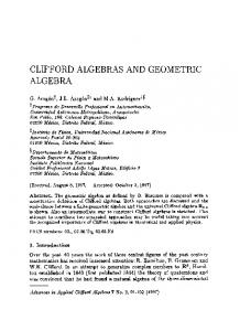
where the integrand contains a finite jump at z = 0, (ρ < L) and no singularities. The integral is simplified by rescaling to give Z ∞ R[(1 + (z + iλ)2 )−1/2 ] , (75) dz 2 W (ρ) = z + 1 + λ2 + [(z 2 + 1 − λ2 )2 + 4λ2 z 2 ]1/2 −∞ where λ = L/ρ > 1. The branch cuts for the complex square roots in this integral follow from the global definition of ω and are shown in Figure 3. The integral is performed by splitting into the two regions z > 0 and z < 0 and rotating each of the contours to lie on the positive imaginary z axis. This leaves six integrals to compute (shown in Figure 3) which combine as follows: I1 + I6 = −2
Z
∞
dy λ+1
y2
λ+1
−
λ2
[(y + λ)2 − 1]−1/2 − 1 + [(y 2 − λ2 − 1)2 − 4λ2 ]1/2
y 2 − λ2 − 1 1 dy 2λ2 λ−1 [(y + λ)2 − 1]1/2 Z λ−1 [(y + λ)2 − 1]−1/2 I3 + I4 = +2 dy 2 . 2 λ + 1 − y + [(y 2 − λ2 − 1)2 − 4λ2 ]1/2 0 I2 + I 5 = −
Z
(76)
These combine into the simpler integrals Z b Z b y 2 − λ2 − 1 1 1 dy dy [(y − λ)2 − 1]1/2 + b→∞ 2λ2 0 2λ2 λ+1 [(y + λ)2 − 1]1/2 Z λ−1 1 − 2 dy [(y − λ)2 − 1]1/2 , (77) 2λ 0
W (ρ) = lim −
12
which are easily evaluated with cosh substitutions. The cutoff b is introduced since the separate integrals are divergent. On performing the substitutions we find that −1 Z Z cosh−1 (b+λ) 1 1 cosh (b+λ) W (ρ) = lim dw coshw− 2 dw sinh2 w b→∞ λ cosh−1 (λ) 2λ cosh−1 (b−λ) ¢ 1 ¡ (b − λ)[(b − λ)2 − 1]1/2 − (b − 3λ)[(b + λ)2 − 1]1/2 = lim 2 b→∞ 4λ 1 − (λ2 − 1)1/2 λ (L2 − ρ2 )1/2 =1− , (78) L so that Z
³ (L2 − ρ2 )1/2 ´ . d3 x ∂a ·T (a) = M 1 − L ρ0 ≤ρ
(79)
Since the solution is axisymmetric, ∂a ·T (a) can only depend on ρ and z. We must therefore have, for ρ < L, ∂a ·T (a) = f (ρ)δ(z),
(80)
where f (ρ) is found from differentiating (79): f (ρ) =
M . − ρ2 )1/2
2πL(L2
(81)
The function f (ρ) is remarkably simple, given the convoluted route by which it is obtained. However, its true significance is not seen until the remaining gauge-invariant information has been extracted from G(a). This information resides in the eigenvalues of G(a), the calculation of which introduces further complexities.
5.2
The Einstein Tensor
To calculate the full form of G(a) over the disk, we start with the most general form that G(a) can take consistent with the fact that the Kerr solution is axisymmetric. Such a form is defined by, for ρ < L, G(γ0 ) = δ(z)[α1 γ0 + β1 φˆ + δ1 eρ + ²1 γ3 ] ˆ = δ(z)[α2 φˆ + β2 γ0 + δ2 eρ + ²2 γ3 ] G(φ)
G(eρ ) = δ(z)[α3 eρ + β3 γ0 + δ3 φˆ + ²3 γ3 ] G(γ3 ) = δ(z)[α4 γ3 + β4 φˆ + δ4 eρ + ²4 γ0 ],
(82)
where each of the αi . . . ²i are scalar functions of ρ only. We do not assume that G(a) is a symmetric linear function so as to allow for the possibility that the matter contains a hidden source of torsion. Calculation of each of the terms in G(a) proceeds in the same manner as the calculation of the Ricci scalar. The resulting computations are long, and
13
somewhat tedious, and have been relegated to Appendix A. The final results are that, for ρ < L, 2M ρ ˆ [ργ0 + Lφ] L(L2 − ρ2 )3/2 2M ˆ = δ(z) ˆ G(φ) [ργ0 + Lφ] (L2 − ρ2 )3/2 2M G(eρ ) = δ(z) eρ 2 L(L − ρ2 )1/2 G(γ3 ) = 0.
G(γ0 ) = −δ(z)
(83)
These confirm that G(a) is symmetric, so there is no hidden torsion. We see immediately that eρ is an eigenvector of G(a), with eigenvalue 2M/[L(L2 − ρ2 )1/2 ], and also that there is no momentum flow in the γ3 direction, which is physically obvious. The structure of the remaining terms is most easily seen by introducing the boost factor λ via tanhλ ≡
cosv coshu
(84)
and defining the timelike velocity ˆ v ≡ eλσ φ γ0 = coshλγ0 + sinhλφ.
(85)
(This second use of the symbol v should not cause any confusion.) With these definitions we see that, over the disk, G(v) = 0, and G(σ φ v) = δ(z)
2M σ φ v. L(L2 − ρ2 )1/2
(86)
(87)
There is therefore zero energy density in the v direction, with isotropic tension of M/[4πL(L2 −ρ2 )1/2 ] in the plane of the disk. This conclusion is gauge invariant, since it is based solely on the eigenvalue structure of the Einstein tensor. It is truly remarkable that such a simple picture emerges from the complicated set of calculations in Appendix A. The velocity vector v defines the natural rest frame in the region of the disk. A second velocity is defined by the timelike Killing vector gt ≡ h−1 (γ0 ) (88) ¯ (see [3] for details of how Killing vectors are handled within gauge-theory gravity.) The boost required to move between these velocities therefore provides an intrinsic definition of the field velocity in the disk region. In this region the ¯ function h(a) reduces to the identity, so gt is simply γ0 . It follows that the velocity is given by tanhλ = cosv = ρ/L, (89) and the angular velocity is therefore 1/L. This is precisely as expected for a rigid rotation, which fits in with the observation of [8] that the Kerr solution can be viewed as the limiting case of a rigidly-rotating matter distribution. 14
5.3
An Alternative Gauge and the Matter Ring
The form of the eigenvectors of G(a) suggest that the more appropriate gauge for the study of the Kerr solution is provided by the boost R ≡ e−λσ φ /2
(90)
so that the new solution is generated by ¯ 0 (a) = R[a + M αa·nn]R. ˜ h
(91)
In this gauge the tension lies entirely in the iσ 3 eigenplane, and the characteristic bivector of the Riemann tensor becomes ˜ = eu (92) Rσ γ R |eu | which is now a relative spatial vector. In this gauge the γ0 frame is the rest frame defined by the Weyl and matter tensors, whereas the Killing vectors are now swept round. The boost (90) is well-defined everywhere except for the ring singularity where the matter is located. This is unproblematic, since the fields are already singular there. We know that the integral of the Ricci scalar over the disk gives Z L ρ = 8πM (93) dρ 8πM 2 − ρ2 )1/2 L(L 0 which accounts for the entire contribution to R found for integrals outside the disk. It follows that the contribution to the stress-energy tensor from the ring singularity must have a vanishing trace, so that no contribution is made to the Ricci scalar. It is also clear that the entire contribution to the angular momentum must come from the ring, since the tension is isotropic over the disk. From these considerations it is clear that the contribution to G(a) from the ring singularity, in the gauge defined by (91), must be of the form Gring (a) =
4M ˆ (γ0 + φ). ˆ δ(z) δ(ρ − L) a·(γ0 + φ) L
(94)
This confirms that the ring current follows a lightlike trajectory — the natural endpoint for collapsing matter with angular momentum. The radius of the orbit, L, agrees with the minimum size allowed by special relativity (see Exercise 5.6 of [9], for example).
5.4
The Physics of the Disk
A natural question is whether the tension field has a simple non-gravitational explanation. This is indeed the case. The equations for a special relativistic fluid are (ε + P )(v·∇v)∧v = ∇P ∧v
∇·(εv) = −P ∇·v,
(95) (96)
where ε is the energy density, P is the pressure and v is the fluid velocity (v 2 = 1). For the case of a ring of particles surrounding a rigidly-rotating 15
massless membrane under tension we see that (ignoring the factors of δ(z)), P = P (ρ) and ˆ v = coshλ γ0 + sinhλ φ, If follows that
ˆ φˆ = − v·∇v = sinh2 λ φ·∇
so the equation for P is
This has the solution
tanhλ = ρ/L.
(97)
ρ eρ , − ρ2
(98)
L2
∂P ρ − 2 P = 0. ∂ρ L − ρ2 P =
P0 , (L2 − ρ2 )1/2
(99)
(100)
which has precisely the functional form of the tension distribution found above. The constant P0 is found by requiring that the trace of the stress-energy tensor returns M when integrated over the disk. This fixes the tension to M/[4πL(L2 − ρ2 )1/2 ], precisely as is built into the gravitational fields. Of course, the required ‘light’ membrane cannot be made from any known matter. Indeed, the fact that the membrane generates a tension whilst having zero energy density means that it violates the weak energy condition. Nevertheless, it is quite remarkable that such a simple physical picture holds in a region of such extreme fields. In writing the tension as M/[4πL(L2 − ρ2 )1/2 ] we are expressing it in terms of the radial coordinate ρ. This coordinate is given physical significance by ¯ function is the identity over the disk region, so ρ is the the fact that the h proper distance from the centre of the disk. This gives a simple gauge-invariant definition of L as the physical radius of the disk. Furthermore, the form of the Riemann tensor (38) shows that its complex eigenvalues are driven by M/ω 3 , which is gauge-invariant, and hence a physically-measurable quantity. This affords gauge-invariant significance to M and ω, and hence to the coordinates ρ and z. It follows that both L and M have simple gauge-invariant definitions, without needing to appeal to the asymptotic properties of the solution.
6
Conclusions
The calculations performed in this paper confirm that the combination of spacetime algebra and the flatspace, gauge-theoretic approach to gravitation provides a powerful new methodology for the analysis of gravitational phenomena. This is exemplified by the demonstration that the complex structure at the heart of vacuum Kerr-Schild fields is the same as the natural complex structure inherent in the Weyl tensor through its self-duality symmetry. Further insights are obtained through the use of null vectors as idempotent elements, simplifying many of the derivations of the vacuum equations. The algebraic advantages of the spacetime algebra approach are seen clearly in equation (34), which gives a remarkably simple and compact expression for the Riemann tensor. The application of Gauss’ theorem in this paper raises a number of questions about the relationship between the gauge-theoretic formulation of gravity and the standard formulation based on differential geometry. We have argued elsewhere [3] that, whilst the approaches agree for common systems of astrophysical 16
interest, differences emerge in more extreme situations. Typically these differences are related to topological considerations, and this is the case for the Kerr solution. According to standard accounts of general relativity [10, 11] if one falls through the ring singularity of a Kerr black hole one ultimately emerges in a new universe — one of an infinite ladder of possible universes connected by a Kerr black hole. Such a situation is possible in standard general relativity because one can continuously patch together separate coordinate systems. The cylindrical Gaussian surfaces used in this paper have no counterpart in such a solution, so it is unclear what the status of the tension field would be. The picture provided by the gauge-theoretic approach is quite different. The ring of matter follows a lightlike trajectory and surrounds a disk of tension. The tension distribution over the disk is precisely that predicted by special relativity. Any particle falling through the ring emerges in the same region of space that is populated by incoming particles from the other side of the hole. The particles then pile up on the inner (Cauchy) horizon, which must be highly unstable. When quantum effects are included the picture is more complicated — the tension over the disk will tear apart any wavepacket, with uncertain consequences. It is also worth noting that the tension field provides an interesting method for pair production by ‘tearing apart’ the vacuum. The fact that the tension membrane violates the weak energy condition raises a further interesting question — how can it be formed from collapsing baryonic matter? Furthermore, if baryonic matter cannot form the membrane, then what is the endpoint of the collapse process? Answers to these questions will only emerge when realistic collapse scenarios are discussed within the gauge-theory gravity framework. There are currently no experimental grounds to choose between our gaugetheoretic approach or conventional general relativity. There is no doubt that the conventional approach to black hole physics is more popular with science fiction writers, but we feel that the pictures provided by the gauge-theoretic approach for both the Reissner-Nordstrom and Kerr solutions have a more physical feel about them. A crucial question to be addressed in future research is whether the differences discussed here could actually have physical consequences for astrophysical rotating black holes with accretion disks. It is known that these spin near the critical rate required for the removal of the horizons. If the horizons were to vanish, leaving a naked singularity, then the presence of the tension disk might be astrophysically testable.
A
Surface Integrals of the Einstein Tensor
From the form of (82) there are 16 scalar functions to find using extensions of the technique described in Section 5.1. These are evaluated below.
A.1
G(γ0 )
For this term we have G(γ0 ) = δ(z)[α1 γ0 + β1 φˆ + δ1 eρ + ²1 γ3 ],
17
(101)
and α1 and ²1 are computed directly from Z ρ Z ¡ ¢ 3 d x G(γ0 ) = 2π dρ0 ρ0 α1 (ρ0 )γ0 + ²1 (ρ0 )γ3 .
(102)
0
ρ0 ≤ρ
On converting to a surface integral we obtain Z 2π Z ∞ Z d3 x G(γ0 ) = ρ dφ dz eρ ·[Ω(γ0 ) − γ0 ∧(∂a ·Ω(a))] ρ0 ≤ρ
0
−∞
2π
Z ∞ 1 dz [(−∂ρ α + (α2 + β 2 )eρ ·n)γ0 + ∂φ β γ3 ] dφ ρ −∞ 0 Z ∞ ¡ L sinhuγγ ∗ ¢ 2 γ0 , (103) = 2πM ρ dz R(γ 3 ) + 2 L cosh2 u −∞ = Mρ
Z
which shows that ²1 = 0. The final term on the right-hand side of (103) is the integral already performed for the Ricci scalar. For the remaining term we need Z ∞ Z ∞ ρ2 dz ρ2 dz R(γ 3 ) = R 2 2 3/2 −∞ −∞ [ρ + (z + iL) ] ¡ ¢ L =2 1− 2 , (104) 2 1/2 (L − ρ ) where it is again crucial that the correct branch cuts are employed in the evaluation of the contour integral. Substituting this result into (103) we find that 2π
Z
ρ 0
¡ dρ0 ρ0 α1 (ρ0 ) = 4πM 2 −
(L2
(L2 − ρ2 )1/2 ¢ L , − 2 1/2 L −ρ )
(105)
and differentiating recovers α1 = −
2M ρ2 . L(L2 − ρ2 )3/2
(106)
For the remaining terms we first observe that Z ρ Z 2 3 ρ d x ρe ·G(γ0 ) = 2π dρ0 ρ0 δ1 (ρ0 ) 0 ρ0 ≤ρ Z ← → d3 x (ρeρ ∧ ∇ )·[Ω(γ0 ) − γ0 ∧(∂a ·Ω(a))] = ρ0 ≤ρ
= 0,
(107)
so we must have δ1 = 0. To find β1 we need to apply the divergence theorem
18
twice: Z ρ Z 2 2π dρ0 ρ0 β1 (ρ0 ) = 0
ˆ d3 x (−ρ0 φ)·G(γ 0) ρ0 ≤ρ 2
= Mρ Z −2
Z
2π
dφ 0
Z
∞
dz (iσ 3 )·(−i∇β) −∞
d3 x (iσ 3 )·[Ω(γ0 ) − γ0 ∧(∂a ·Ω(a))] Z → − 2 = 2πM ρ [β(0− ) − β(0+ )] + 2M d3 x (iσ 3 )·[∇·(αn)n] ρ0 ≤ρ
ρ0 ≤ρ
2
=−
4πM ρ + 4πM ρ − ρ2 )1/2
(L2
Z
∞
dz −∞
α cosv coshu
4πM ρ2 + 8πM LW (ρ), =− 2 (L − ρ2 )1/2
(108)
with W (ρ) as given by equation (78). This time, differentiating yields β1 = −
(L2
2M ρ . − ρ2 )3/2
(109)
Reassuringly, this term vanishes on the axis, as it must do for a valid axiallysymmetric solution.
A.2
G(γ3 )
For G(γ3 ) we can write G(γ3 ) = δ(z)[α4 γ3 + β4 φˆ + δ4 eρ + ²4 γ0 ]. This time we find that Z Z ρ 0 0 0 0 2π dρ ρ [α4 (ρ )γ3 + ²4 (ρ )γ0 ] = 0
(110)
d3 x G(γ3 )
ρ0 ≤ρ
= −2πM ργ0 + M ργ3
Z
0
∞
Z
dz ∂ρ (ασ 3 ·n) −∞ 2π Z ∞ dφ Z
= −2πM ργ0 ∂ρ = 0.
dz (−iσ φ )·[−i∇(βσ 3 ·n)]
−∞ ∞
dz α sinv
−∞
(111)
The final term vanishes because α sinv is an odd function of z. It follows that α4 = ²4 = 0. The same argument as at equation (107) shows that δ4 = 0, and
19
for β4 we construct Z Z ρ 0 02 0 2π dρ ρ β4 (ρ ) = 0
ˆ d3 x (−ρ0 φ)·G(γ 3) ρ0 ≤ρ
= M ρ2 Z −2
Z
2π
dφ 0
Z
∞
dz (iσ 3 )·[−i∇(βσ 3 ·n)]
−∞
d3 x (iσ 3 )·[Ω(γ3 ) − γ3 ∧(∂a ·Ω(a))]
ρ0 ≤ρ
Z
2π
Z
∞
dz (iσ 3 )·[−α(iσ φ )·nn] dφ = −2M ρ −∞ 0 Z ∞ α sinv cosv dz = 4πM ρ coshu −∞ = 0,
(112)
where we have again used the fact that sin v is an odd function of z. We therefore have G(γ3 ) = 0, which is physically reasonable.
A.3
ˆ G(eρ ), G(φ)
For these terms we write ˆ = δ(z)[α2 φˆ + β2 γ0 + δ2 eρ + ²2 γ3 ] G(φ) G(eρ ) = δ(z)[α3 eρ + β3 γ0 + δ3 φˆ + ²3 γ3 ].
(113) (114)
The calculations are now complicated by the fact that the vector arguments are functions of position. To get round this problem we must find equivalent integrals in terms of the fixed γ1 and γ2 vectors. We first form Z ρ 2 2π dρ0 ρ0 ²2 (ρ0 ) 0 Z ˆ = d3 x (−ρ0 γ3 )·G(φ) ρ0 ≤ρ
Z 2π Z ∞ ˆ − φ∧(∂ ˆ = M ρ2 dφ dz (−iσ φ )·[Ω(φ) a ·Ω(a))] 0 −∞ Z ¡ ¢ + d3 x (iσ1 )·[Ω(γ1 ) − γ1 ∧(∂a ·Ω(a))] + (iσ2 )·[Ω(γ2 ) − γ2 ∧(∂a ·Ω(a))] ρ0 ≤ρ
= −2πM ρ2
Z
∞
dz −∞
β sinhu cosv + 2πM ρ coshu
Z
∞
dz −∞
α sinv cosv coshu
=0
(115)
which shows that ²2 = 0. A similar calculation confirms that ²3 = 0.
20
If G(a) is symmetric then we expect to find β2 = −β1 . This is confirmed by Z ρ 2 2π dρ0 ρ0 β2 (ρ0 ) Z 0 ˆ = d3 x ρ0 γ0 ·G(φ) =ρ
ρ0 ≤ρ Z 2π 2
dφ
0
−
Z
Z
∞
ˆ − φ∧(∂ ˆ dz eρ ·[Ω(φ) a ·Ω(a))]
−∞
¡ ¢ d3 x σ1 ·[Ω(γ2 ) − γ2 ∧(∂a ·Ω(a))] − σ2 ·[Ω(γ1 ) − γ1 ∧(∂a ·Ω(a))]
ρ0 ≤ρ
= 2πM ρ2 ∂ρ
Z
∞
dz −∞
α cosv − 2πM ρ coshu
Z
∞
dz −∞
α cosv coshu
2
= 4πM Lρ ∂ρ (W (ρ)/ρ) − 4πM LW (ρ) = −8πM LW (ρ) +
4πM ρ2 . − ρ2 )1/2
(116)
(L2
A similar, though slightly more involved calculation confirms that β3 = 0. For the remaining four functions we need to consider various combinations of integrals. For example, Z Z ρ 0 0 0 0 d3 x γ 1 ·G(γ1 ) π dρ ρ (α2 (ρ ) + α3 (ρ )) = ρ0 ≤ρ
0
= Mρ
Z
2π
dφ 0
Z
∞
dz sinφ(−iσ 3 )·[−i∇(βσ1 ·n)]
−∞
πρ2 M [β(0+ ) − β(0− )] L 2πM ρ2 = , L(L2 − ρ2 )1/2
=
(117)
from which we obtain α2 + α 3 =
L(L2
Similarly, Z Z ρ 0 0 0 0 π dρ ρ (δ2 (ρ ) − δ3 (ρ )) = 0
4M 2M ρ2 + . 2 1/2 −ρ ) L(L2 − ρ2 )3/2
(118)
d3 x γ 1 ·G(γ2 )
ρ0 ≤ρ
= Mρ
Z
2π
dφ 0
=0
Z
∞
dz sinφ (−iσ 3 )·[−i∇(βσ 2 ·n)]
−∞
(119)
(because sinhu = 0 over the disk). This result confirms that G(a) is symmetric over the disk and therefore that there are no hidden sources of torsion.
21
The functions δ2 and δ3 are obtained from Z Z ρ π 2 3 d3 x ρ0 sinφ cosφ γ1 ·G(γ1 ) dρ0 ρ0 (δ2 (ρ0 ) + δ3 (ρ0 )) = 4 0 0 ρ ≤ρ Z 2π Z ∞ = M ρ3 dφ dz sin2 φ cosφ(iσ 3 )·[−i∇(βσ1 ·n)] 0 −∞ Z − d3 x ρ0 cosφ (iσ 3 )·[Ω(γ1 ) − γ1 ∧(∂a ·Ω(a))] ρ0 ≤ρ
= −M ρ2
Z
2π
dφ 0
Z
∞
dz sinφ cosφ α(iσ 3 ∧n)2
−∞
= 0,
(120)
which shows that δ2 = δ3 = 0. It follows that eρ is an eigenvector of the stress-energy tensor. A similar trick is used to evaluate the final term: Z Z π ρ 0 03 2 0 0 dρ ρ (α2 (ρ ) − α3 (ρ )) = d3 x ρ0 sinφ cosφ γ1 ·G(γ2 ) 4 0 0 ρ ≤ρ Z 2π Z ∞ = M ρ3 dφ dz sin2 φ cosφ(iσ 3 )·[−i∇(βσ 2 ·n)] 0 −∞ Z d3 x ρ0 cosφ(iσ 3 )·[Ω(γ2 ) − γ2 ∧(∂b ·Ω(b))] − ρ0 ≤ρ
=
πM ρ4 − 2πM ρ2 W (ρ) 2L(L2 − ρ2 )1/2 Z ρ + 4πM dρ0 ρ0 W (ρ0 ),
(121)
0
where W (ρ) is as defined in equation (78). We do not need to evaluate the final integral since we are only interested in the derivative of the right-hand side. This yields 2M ρ2 α2 − α 3 = (122) L(L2 − ρ2 )3/2 which now gives us all of the terms in G(a).
References [1] C.J.L. Doran. Integral equations and Kerr-Schild fields I. Sphericallysymmetric fields. gr-qc ?, 1997. [2] A.N. Lasenby, C.J.L. Doran, and S.F. Gull. Astrophysical and cosmological consequences of a gauge theory of gravity. In N. S´anchez and A. Zichichi, editors, Advances in Astrofundamental Physics, Erice 1994, page 359. World Scientific, Singapore, 1995. [3] A.N. Lasenby, C.J.L. Doran, and S.F. Gull. Gravity, gauge theories and geometric algebra. To appear in Phil. Trans. R. Soc. Lond. A, 1997. [4] M.M. Schiffer, R.J. Adler, J. Mark, and C. Sheffield. Kerr geometry as complexified Schwarzschild geometry. J. Math. Phys., 14(1):52, 1973. 22
[5] E.T. Newman and A.I. Janis. Note on the Kerr spinning-particle metric. J. Math. Phys., 6(4):915, 1965. [6] C. Pichon and D. Lynden-Bell. New sources for the Kerr and other metrics: Rotating relativistic discs with pressure support. Mon. Not. R. Astron. Soc., 280:1007, 1996. [7] G. Neugebauer and R. Meinel. The Einsteinian gravitational field of the rigidly rotating disk of dust. ApJ, 414:L97, 1993. [8] F.J. Chinea and L.M. Gonzalez-Romero. A differential form approach for rotating perfect fluids in general relativity. Class. Quantum Grav., 9:1271, 1992. [9] C.W. Misner, K.S. Thorne, and J.A. Wheeler. Gravitation. W.H. Freeman and Company, San Francisco, 1973. [10] S.W. Hawking and G.F.R. Ellis. The Large Scale Structure of Space-Time. Cambridge University Press, 1973. [11] W.J. Kaufmann. The Cosmic Frontiers of General Relativity. Penguin Books, 1979.
23
Figure 1: Two views of the integral curves of n. The top figure shows the view from above of a set of incoming geodesics that terminate along a diameter of the central disk. This pattern is rotated around the z-axis to give the full set of geodesics. The lower figure shows incoming geodesics from above and below the disk. These are the mirror image of each other. The ring is shown for convenience — it is not an integral curve of n.
24
3
2
1
00
2
1
3
4
5
-1
-2
-3
4
2
-1
00
1
2
3
4
5
-2
-4
Figure 2: The complex function ω for fixed ρ as a function of z. In both cases L = 1. Figure (a) is for ρ = 2 > L and the right-hand side for ρ = 0.5 < L. The solid lines are for ω 2 and the broken lines for the square root. Continuity of ω for finite z requires that ω be discontiuous over the central disk.
25
λ+1 λ−1 −(λ − 1)
−(λ − 1)
−(λ + 1)
−(λ + 1)
[1 + (z + iλ)2 ]1/2
[(z 2 + 1 − λ2 )2 + 4λ2 z 2 ]−1/2 I1
I6
I2
I5
I3
I4
Figure 3: Branch cuts and contours for the integral (75). The branch cuts for complex z shown in the top two figures follow from the global definition of ω. The bottom figure shows the six integrals that have to be calculated after the integration contour has been rotated.
26