mented via a projection formula by the max-function. Secondly ..... tively, and fem.bnd.r and fem.bnd.g correspond to Gl and Rm when defining the. PDEs and the ...
STRATEGIES FOR TIME-DEPENDENT PDE CONTROL WITH INEQUALITY CONSTRAINTS USING AN INTEGRATED MODELING AND SIMULATION ENVIRONMENT. (AUTHORS VERSION. THE ORIGINAL PUBLICATION IS AVAILABLE AT WWW.SPRINGERLINK.COM.)
IRA NEITZEL∗ , UWE PRÜFERT
F
AND THOMAS SLAWIG�
Abstract. In [17] we have shown how time-dependent optimal control for
partial di�erential equations can be realized in a modern high-level modeling and simulation package. constrained problems.
In this article we extend our approach to (state)
�Pure� state constraints in a function space setting
lead to non-regular Lagrange multipliers (if they exist), i.e.
the Lagrange
multipliers are in general Borel measures. This will be overcome by di�erent regularization techniques. To implement inequality constraints, active set methods and barrier methods are widely in use.
We show how these techniques can be realized in a
modeling and simulation package. We implement a projection method based on active sets as well as a barrier method and a Moreau Yosida regularization, and compare these methods by a program that optimizes the discrete version of the given problem.
1. Introduction In this paper we show how time-dependent optimal control problems (OCP) subject to point-wise state constraints can be solved using an equation based integrated modeling and simulation environment (IMSE) like e.g.
Comsol Multiphysics,
Pdetool, or OpenFoam. We extend the approach from [17] where we considered time-dependent OCPs without inequality constraints. There we focused on two possible methods to deal with reverse time directions appearing in the optimality systems: A somehow �classical� iterative approach based on subsequently solving the forward state and the backward adjoint equation and an alternative approach transforming the complete optimality system into a coupled elliptic system by interpreting time as an additional space dimension. In this paper we focus on the latter approach. Throughout this paper we consider optimal control problems
(1)
min j(y, u)
Key words and phrases.
=
θQ θΩ ky(T ) − yΩ k2L2 (Ω) + ky − yQ k2L2 (Q) 2 2 κΣ κQ + kuΣ k2L2 (Σ) + kuQ k2L2 (Q) 2 2
Optimal control, parabolic PDEs, inequality constraints, integrated
modeling and simulation environments.
> Research supported by the DFG Schwerpunktprogramm SPP 1253, F Research supported by the DFG Research Center Matheon, � Research supported by the DFG Cluster of Excellence The Future Ocean and the DFG Schwerpunktprogramm SPP 1253.
1
subject to the parabolic PDE
(2)
yt − ∇ · (∇y)
= βQ uQ + f
in
Q
~n · ∇y + αy
= βΣ uΣ + g
on
Σ
in
Ω
y(0)
= y0 1
and to the (lower) unilateral constraints
ya ≤ τ y + λuQ
(3)
a.e. in
Q.
In the following, we refer to the parabolic PDE (2) as the state equation. We consider only the case
τ ≥ 0, λ ≥ 0
and
τ + λ > 0.
The setting
τ > 0, λ > 0
implements mixed control-state constraints. For this class of problems, the existence of Lagrange multipliers is often shown by Slater point arguments. Therefore, the state is considered in the space of continuous functions. Due to parabolic regularity theory this can only be expected in the case of one dimensional distributed controls unless higher regularity of controls can be assumed.
Even then, caused by the
fact that for �pure� state constraints the associated Lagrange multipliers are i.g. Borel measures, regularization techniques can improve the behavior of numerical algorithms, cf. [13], [8], or [1]. For constraints given on the same domain as the control we can use the well investigated Lavrentiev-type regularization, see e.g. the works [14] or [19].
In the case of boundary control and constraints given on the
space-time domain the Lavrentiev regularization cannot be applied.
Here, some
di�erent regularization concepts have been developed, examples can be found in [24] and [9] for elliptic problems and [18] for parabolic PDE control. Alternatively, for distributed as well as for boundary controlled problems, the Moreau-Yosida regularization suggested in [8] may be applied. The structure and underlying theory of the optimal control problem should be kept in mind when considering appropriate discretization schemes. In most FEM packages and IMSEs an adequate implementation of regular measures is not possible. Of course, one can try to approximate measures by �nite elements or discretize them by point-wise evaluations [5], but our aim is to implement optimality conditions (and solve optimal control problems) without additional programming e�ort. Therefore, measures should be avoided, and we will mainly consider regularized problem formulations in our experiments, that o�er the additional bene�t that Lagrange multipliers exist without any further restrictions. In this paper, we investigate some methods to handle state constraints. First, we use the regularization suggested in [18] in the parabolic boundary controlled case and the classical Lavrentiev-type regularization as discussed in [14] in the case of distributed control. The optimality system can in this case be implemented via a projection formula by the max-function. Secondly, we test some barrier methods to eliminate the point-wise state constraints. In [21], it is shown that under certain assumptions barrier methods do not need any additional regularization if their order is su�ciently high and the solutions of the state equations are su�ciently smooth. In this sense, barrier methods regularize the problem �by default�. The integration of a path-following algorithm into the framework established in [17] needs only minor changes in comparison to the solution of problems without inequality constraints. Another possible way to overcome the lack of regularity of Lagrange multipliers is the Moreau-Yosida approximation of the Lagrange multipliers, cf. [8], which we also apply to some examples.
1In
this paper, we only consider unilateral constraints of lower type
for upper constraints
βy + γu ≤ yb
is completely analogous.
2
ya ≤ βy + γu.
The theory
This paper is organized as follows: In Section 2 we specify the optimality conditions and quote some results concerning the existence and uniqueness of a minimizer for the given class of problems. In the following Section 3 we introduce regularization techniques to avoid measures as Lagrange multipliers and ensure the existence of multipliers.
In Section
4 we describe di�erent methods to handle inequality constraints algorithmically, followed by the implementation of these algorithms in Section 5 using Comsol
Multiphysics as a concrete example for an IMSE. In Section 6 some examples illustrate the properties of our approach. 2. Optimality conditions for problems with inequality constraints
Assumption 2.1.
Let
Ω ⊂ RN , N ∈ N,
be a bounded domain with
C 0,1 -
∂Ω if N ≥ 2, and a bounded interval in R if N = 1. Moreover, for ¯ , Q = Ω × (0, T ), Σ = ∂Ω × (0, T ) let functions f ∈ L2 (Q), g ∈ L2 (Σ), y0 ∈ C(Ω) 2 2 yQ ∈ L (Q), and yΩ ∈ L (Ω) be given. Further, we have real numbers α, βQ , βΣ , and non-negative numbers θQ , θΩ , κQ , and κΣ . The constraint is a function in ¯ with y0 (x) > ya (x, 0). C(Q) Note, that the following assertions hold valid if we replace the −∇ · ∇-operator ∞ in (2) by a more general elliptic operator −∇ · A∇y + a0 y , where a0 ∈ L (Q), and 1,γ A = (aij (x)), i, j = 1, ..., N is a symmetric matrix with aij ∈ C (Ω), γ ∈ (0, 1), that satis�es the following condition of uniform ellipticity: There is an m > 0 such
boundary
that
ξ > A(x)ξ
≥ m|ξ|2
for all
ξ ∈ RN
and all
¯ x ∈ Ω.
In the following we give a brief survey on known results concerning existence and regularity of solutions of parabolic PDEs as well as on the existence of an optimal solution of the control problem. Further, we specify the necessary optimality conditions for the considered cases.
De�nition 2.2 We de�ne the solution space for the state equation (2) by W (0, T ) = {y ∈ L2 (0, T ; H 1 (Ω)) | yt ∈ L2 (0, T, H 1 (Ω)∗ )}.
Theorem 2.3.
the initial value problem (2)
c>0
(βQ uQ + f, βΣ uΣ + g, y0 ) ∈ L2 (Q)×L2 (Σ)×L2 (Ω) admits a unique solution y ∈ W (0, T ). There exists a
For any triple
such that
kykW (0,T ) ≤ c kβQ uQ + f kL2 (Q) + kβΣ uΣ + gkL2 (Σ) + ky0 kL2 (Ω)
�
holds true. For the proof we refer to [26], [11], or [12].
Theorem 2.4. Let Ω be a bounded domain with C 1,1 -boundary. Further let (βQ uQ +f, βΣ uΣ +g, y0 ) ∈ Lp (Q)×Lq (Σ)×L∞ (Ω) be given. For every p > N/2+1 ∞ ¯ for all and s > N + 1, the weak solution of (2) belongs to L (Q) ∩ C([δ, T ] × Ω) δ > 0. There is a constant c not depending on (uQ , uΣ , f, g), such that kykL∞ (Q) ≤ ckβQ uQ + f kLp (Q) + kβΣ uΣ + gkLq (Σ) + ky0 kL∞ (Ω) holds true. If
¯ , y0 ∈ C(Ω)
then
¯ . y ∈ C(Q)
For a proof we refer to [20, Prop. 3.3] or [4] Depending on the choice of the parameters
κQ , κΣ , βQ ,
and
βΣ
the following
meaningful constellations are possible:
κΣ = 0, βΣ = 0, κQ > 0, βQ 6= 0,
then
u := uQ ,
κQ = 0, βQ = 0, κΣ > 0, βΣ 6= 0,
then
u := uΣ ,
(1) distributed control: Let
U := L2 (Q) (2) boundary control: Let
U := L2 (Σ) 3
κQ > 0, βQ 6= 0, κΣ > 0, βΣ 6= 0, u = (uQ , uΣ ). U := L2 (Q) × L2 (Σ),
(3) boundary and distributed control: Let then where
U
denotes the space of controls.
In our numerical experiments we will consider either distributed or boundary controlled problems.
Theorem 2.5.
Let Assumption 2.1. hold. For each of the cases 1�3, Problem
u∗ ∈ U
(1)�(3) has a unique solution
with associated state
y ∗ ∈ W (0, T ).
For a proof we refer to [23]. In order to formulate �rst order necessary optimality conditions, we rely on the continuity of the optimal state. In contrast to elliptic PDEs here the necessity of continuous states is a stronger restriction. In the case of boundary control, we have
βΣ uΣ + g ∈ L2 (Σ), so that the assumption q > N + 1 of Theorem 2.5 is not ful�lled for q = 2. In the case of distributed control, for space dimension N > 1 the assumption p > N/2 + 1 is not ful�lled for p = 2. In both cases, we do not have the necessary regularity of the state y . To obtain optimality conditions or Lagrange ¯ , hence multipliers at all, we have to claim that the optimal state belongs to C(Q)
only
we rely on the following assumption.
Assumption 2.6.
Either
p
and
Let �pure� state constraints be given.
N = 1 or the control q su�ciently large.
is su�ciently regular, i.e.
Then we demand:
uQ ∈ Lp
and
uΣ ∈ Lq
with
Later we will see that regularization techniques will help to avoid this regularity problem. 2.1.
Control constraints.
Setting
τ = 0 and λ = 1, ya ≤ u .
the mixed control-state
constraint (3) becomes a control constraint
Theorem 2.7.
optimal state
y
∗
Let
. The
u∗ be the optimal solution to problem (1)�(3) with associated adjoint state p is the solution of the adjoint equation
−pt − ∇ · (∇p)
= θQ (y ∗ − yQ )
in
~n · ∇p + αp = 0 p(T ) = θΩ (y ∗ (T ) − yΩ ) Further,
u∗
Q Σ Ω.
on in
satis�es the projection formula
u∗ =
max{ya , − κβQ p} Q
in
Q
if
κQ > 0
max{ya , − κβΣΣ p}
on
Σ
if
κΣ > 0.
The proof of this theorem can be found e.g. in the monograph [23]. The numerical treatment of control constrained problems is widely discussed in the literature, cf. [6], [2], [10], so we abstain from giving examples. Although we do not speci�cally deal with purely control constrained problems, these optimality conditions are the basis of the derivation of optimality systems in the case of Lavrentiev-type regularized problems. cf. [15]. 2.2.
Pure state constraints. ya ≤ y . ∗ Let u be
Setting
λ=0
and
τ = 1,
the constraint becomes a
pure state constraint
Theorem 2.8.
the optimal solution of problem (1)�(3) that ful�lls
¯ . Then there exist an y ∗ ∈ C(Q) ¯ × (0, T ]), µ = µQ + µΣ + µΩ , µ ∈ B(Ω
the Assumption 2.6. with associated optimal state adjoint state
p
and a regular Borel measure
that together with
u∗
and
y∗
ful�ll the adjoint equation
−pt − ∇ · (∇p) ~n · ∇p + αp p(T )
= θQ (y ∗ − yQ ) − µQ = −µΣ
Q
on
∗
= θΩ (y (T ) − yΩ ) − µΩ 4
in
in
Σ
Ω,
the gradient equation
( 0
=
κQ u∗ + βQ p
in
Q
if
κQ > 0
κΣ u∗ + βΣ p
on
Σ
if
κΣ > 0
and the complementary slackness conditions
ZZ
(y ∗ − ya ) dµ(x, t)
=
0
¯ Q
µ ≥ 0 ¯ y ∗ (x, t) − ya (x, t) ≥ 0 ∀ (x, t) ∈ Q. For a proof we refer to e.g. [20, 4]. Note, that due to Assumption 2.1 we have
µ|Ω×{0} = 0 since y0 (x) > ya (x, 0). Note again, that without assumptions on the ¯ dimension N or the regularity of the optimal control, optimality conditions cannot generally be shown. This can be overcome for instance by the regularization techniques presented in the following sections. We will also see that then the regularity of the multipliers can be improved so that the use of standard discretization schemes in an IMSE is justi�ed.
3. Regularization of state constraints 3.1.
Mixed control-state constraint.
λ > 0 and τ > 0 be given. This mixed τ � λ > 0 as
Let
control-state constraint can be seen as model-given or in the case of
regularization of pure state constraints by perturbation of the state constraint by a small quantity of the control. This technique is known under the term Lavrentiev-
type regularization, cf.
[14].
Without loss of generality, we scale the constraints
τ = 1, λ > 0. Theorem 3.1. Let u∗ be the optimal solution of problem (1)�(3) with associated ∗ optimal state y ∈ W (0, T ). Then there exist an adjoint state p ∈ W (0, T ) and a 2 Lagrange multiplier µ = µQ ∈ L (Q) such that the adjoint equation
such that
−pt − ∇ · (∇p) ~n · ∇p + αp
= θQ (y ∗ − yQ ) − µQ
in
= θΣ (y ∗ − yΣ )
on
Σ
in
Ω,
∗
= θΩ (y (T ) − yΩ )
p(T )
Q
the gradient equation
( 0
=
κQ u∗ + βQ p
in
Q
if
κQ > 0
κΣ u∗ + βΣ p
on
Σ
if
κΣ > 0,
and the complementary slackness conditions
ZZ
(y ∗ + λu∗ − ya ) µQ dxdt =
0
¯ Q
µQ y + λu − ya ∗
∗
≥ 0 ≥ 0
a.e. in a.e. in
Q Q
are satis�ed. For a proof we refer to [15]. Note, that no additional assumptions on the control or dimensions are necessary.
5
3.2.
Problem case: state constraints in the domain and boundary control.
One standard problem belonging to this class is the following:
min j(y, u)
(4)
κΣ θQ ky − yQ k2L2 (Q) + kuΣ k2L2 (Σ) 2 2
=
subject to the boundary controlled PDE
yt − ∇ · (∇y)
=
0
~n · ∇y + αy = αuΣ y(0) = y0
(5)
in
Q
on
Σ Ω
in
and to the point-wise constraints in the interior of the space-time domain
ya ≤ y
(6)
a.e. in
Q
In that case we cannot generally expect existence of a Lagrange multiplier, not even in the space of regular Borel measures. The standard Lavrentiev regularization cannot be applied because the control
u is not de�ned in Q.
Here, the new approach
in [24] (for an elliptic PDE) or [18] (for a parabolic PDE) will help to overcome this problem.
The source-term representation The idea behind this regularization is to introduce an auxiliary distributed con-
v which is coupled with u by an adjoint equation, u = S ∗ v , where S denotes the ∗ solution operator of the state equation and S its adjoint. Here, w is the solution of the adjoint equation and u its trace, cf. [18].
trol
We replace (4)�(6) by the problem (7)
min j(y, w, v)
=
θQ κΣ � ky − yQ k2L2 (Q) + kαwk2L2 (Σ) + kvk2L2 (Q) 2 2 2
subject to the state equation
yt − ∇ · (∇y)
=
0 2
~n · ∇y + αy = α w y(0) = y0
(8)
in
Q
on in
Σ Ω,
in
Q
on
Σ Ω
to the additional equation
−wt − ∇ · (∇w)
= v
~n · ∇w + αw = 0 w(T ) = 0
(9)
in
and to the state constraints with modi�ed Lavrentiev-type regularization
ya ≤ y + λv
(10)
a.e. in
Q.
� is chosen � = c0 λ1+c1 , c0 > 0 and 0 ≤ c1 < 1. Theorem 3.2. Let (y∗ , v∗ , w∗ ) be the optimal solution of (7)�(10). Then there 2 exist adjoint states p, q ∈ W (0, T ), and a Lagrange multiplier µQ ∈ L (Q) such In [18] convergence for vanishing Lavrentiev parameters is shown if
according to
that the state and the adjoint equation
yt − ∇ · (∇y ∗ ) ∗
~n · ∇y + αy
∗
y ∗ (0) −pt − ∇ · (∇p) (11)
=
0
= α
2
∗ wΣ
= y0
in
Q
on
Σ Ω
in
= θQ (y ∗ − yQ ) − µQ
~n · ∇p + αp = 0 p(T ) = 0
in
Q
on in
6
Σ Ω,
the control and the second adjoint equation
−wt − ∇ · (∇w∗ ) ∗
~n · ∇w + αw
∗
∗
w (T ) qt − ∇ · (∇q)
1 λ = − q + µQ � � = 0 =
=
in
∗ (κΣ wΣ
Σ Ω
in
0 2
Q
on
0
~n · ∇q + αq = α q(0) = 0
(12)
in
+ p)
on
a.e. in
Q,
Q
Σ in Ω,
the gradient equation
�v ∗ + q − λµQ
(13)
=
0
and the complementary slackness conditions
RR
(y ∗ + λv − ya ) µQ dxdt =
0
Q
(14)
≥ 0 ≥ 0
µQ y ∗ + λv ∗ − ya
a.e. in a.e. in
Q Q
hold. The proof is given in [18]. Here, the Lagrange multiplier is a regular
L2 -function
without additional assumptions. Note, that the equations (9) and (12) are of the same type as the state equation (8) and the adjoint equation (11). 3.3.
Moreau-Yosida regularization.
The Moreau Yosida regularization, cf. e.g.
[8], replaces the state constraint by a modi�ed objective functional. We consider only the case with state constraints given on the space-time domain
Q.
The problem
reads now minj(y, u)
θQ θΩ ky(T ) − yΩ k2L2 (Ω) + ky − yQ k2L2 (Q) 2 2 κQ κΣ + kuk2L2 (Q) + kuk2L2 (Σ) 2 ZZ 2 1 2 + (γ (ya − y) + µ ¯Q )+ dxdt 2γ
=
(15)
Q subject to the state equation (2). This method is referred as penalization, the last integral in (15) is called a penalty term. Here,
µ ¯Q
is an arbitrary function that belongs to
L2 (Q)
and
γ ∈ R, γ � 1
is a
regularization parameter. We obtain the Moreau-Yosida regularized multiplier
which is an object from
µQ = max{0, µ ¯Q + γ (ya − y)}, L (Q). Note that this regularization 2
approach works with-
out additional PDEs even for boundary control problems. 4. Algorithms to handle state constraints 4.1.
The projection method.
The projection method replaces the complemen-
tary slackness conditions by a projection. This can be viewed as an implementation of the well known active set strategy as a semi-smooth newton method, cf. [7]. In this sense it is possible to show that the complementary slackness conditions (14) are equivalent to
µQ = max {0, µQ + c (ya − λv ∗ − y ∗ )} , 7
for an arbitrarily chosen �xed
c > 0.
boundary-controlled case. Choosing
1 ∗ λ (�v + q) in the as in [24], we obtain a projection
Equation (13) yields
� λ2
c=
>0
µQ =
formula for the Lagrange multiplier
� � 1 ∗ max 0, q + 2 (ya − y ) λ λ �
µQ
(16)
=
a.e. in
Q.
Now, we have to solve an optimality system consisting of the PDEs (8), (11), (9), and (12), and the projection equation (16).
In Section 5.1 we present some
details of the implementation of this method in a Comsol Multiphysics-script. Note, that for distributed control the approach leads to
� � 1 κ µQ = max 0, p + 2 (ya − y ∗ ) λ λ
(17) 4.2.
Q.
a.e. in
The Moreau Yosida regularization by Ito and Kunisch.
From Section
3.3 we obtain the optimality system
yt − ∇ · (∇y)
= βQ uQ + f
in
Q
~n · ∇y + αy
= βΣ uΣ + g
on
Σ
in
Ω
y(0) −pt − ∇ · (∇p)
= y0
= θQ (y − yQ ) − µQ
~n · ∇y + αy = 0 y(T ) = θΩ (y(T ) − yΩ ) µQ = max{0, γ(ya − y)} ( 0 where we choose
=
µ ¯ Q ≡ 0.
in
Q Σ Ω
on in
Q
κQ u∗ + βQ p
in
Q
if
κQ > 0
κΣ u∗ + βΣ p
on
Σ
if
κΣ > 0
For a proof
in
of the validity of the optimality system
and for further details see [8] for the elliptic case. We implement this method by a semi-smooth Newton method in Section 5.1. 4.3.
The barrier method.
Barrier methods replace the inequality constraints by
adding an arbitrary barrier (or penalty) term to the objective functional.
De�nition 4.1. For all
q≥1
g(z; ν; q) : R+ → R ∪ {+∞} −ν ln(y − ya ) :q=1 νq g(y; ν; q) := :q>1 (q − 1)(y − ya )q−1
and
ν>0
the function
is called barrier function of order
q.
de�ned by
The barrier functional is de�ned by
Z b(y; ν, q) :=
g(y; ν, q) dxdt. Q
We can now rede�ne our basic problems without any constraints. Let be barrier functions to the given inequality constraints.
gi (zi ; ν; q)
Then we eliminate all
constraints by de�ning the new problem
min f (y, u) = j(y, u) + b(y; ν, q)
(18)
subject to (2) and (3). The presence of (3) is necessary because:
•
if
q = 1,
the barrier function is not de�ned if
with measure greater zero.
8
y − ya < 0
on a subset of
Ω
•
if
q > 1,
g has �nite values on infeasible points, hence it is not a barrier
function. Another way to handle this problem is introducing an indicator function with respect to the feasible set, cf. [21]. First we observe that every pair
(y, u)
respect to the inequality constraints. lower semi-continuous. For
ν→0
that holds
f (y, u) < ∞ is feasible with f is coercive, convex, and
The functional
this optimal control problem is equivalent to the
problem (1) with pure state constraints. In our numerical tests we will use logarithmic barrier functionals. This choice is based on [21, Lemma 6.1.] and the following remarks. By the assumed regularity of the optimal state [21, Lemma 6.1.] provides the strict feasibility of the solution
(yν , uν )
of (18). Then the objective is directional di�erentiable at
(yν , uν )
and the
following theorem holds:
Theorem 4.2.
For �xed
ν > 0 let uν be the optimal solution of Problem yν . Then there exists an adjoint state p such
with associated optimal state
(18) that
the �rst order optimality conditions
−pt − ∇ · (∇p)
= θQ (yν − yQ ) −
~n · ∇p + αp
=
ν yν − ya
in
0
on
= θΩ (yν (T ) − yΩ )
p(T )
Q
in
Σ
Ω,
and
( 0
κQ uν + βQ p
in
Q
if
κQ > 0
κΣ uν + βΣ p
on
Σ
if
κΣ > 0
=
hold. We use the last theorem to implement the path-following Algorithm 1.
Algorithm 1 Path-following Choose
ν0 , 0 < σ < 1, Set k = 0.
and
Choose some initial values for
δ > 0. y k , u k pk
νk > eps
while
solve the optimality system by Newton's method with initial value
(yk , uk , pk )
up to an accuracy
δ.
νk+1 = νk · σ , set k = k + 1;
set
end
Remark 4.3.
For �xed
νk
[21, Theorem 4.1] provides a unique solution.
To
�nd that solution, we have to solve the optimality conditions given by Theorem 4.2. In the spirit of [17], we want to do this by using an IMSE to solve the optimality conditions, i.e. a system of non-linear coupled PDEs, by Newton's method. Unfortunately, we have no information concerning the convergence radius of Newton's method, so we cannot ensure the convergence of the path-following method. However, if we �nd a solution for some by setting
νk = σνk−1 .
ν0 ,
we can decrease the path parameter
In the worst case, this
σ
ν
will be almost one. For further
details we refer to [25, 19], and [21]. 4.4.
Pros and cons of regularization.
The Lavrentiev-type regularization dis-
cussed in Section 3.1, the regularization for boundary controlled problems with distributed state constraints from Section 3.2, as well as the Moreau-Yosida regularization lead to well-posed problems in numerous ways.
9
•
First of all, only functions of at least
L2 -regularity
are involved in the
optimality systems. Therefore, we do not need special techniques to handle measures in discrete systems.
•
This may lead to an improvement of the numerical treatment, i.e.
the
Lagrange multipliers can be discretized without additional e�ort.
•
Moreover, Lagrange multipliers exist for arbitrary spatial dimensions without additional assumptions on the optimal control.
On the other hand, some disadvantages have to be mentioned:
•
Feasible solutions with respect to the mixed control state constraints
y + λu are in general infeasible with respect to the ya ≤ y . This behavior is known under the term
ya ≤
original state constraint �relaxation of the state
constraints�.
•
For boundary controlled systems, the source-term representation leads to a system that contains two additional PDEs, hence the numerical e�ort grows signi�cantly. The Moreau-Yosida regularization avoids this disadvantage.
•
The choice of parameters is di�cult for all methods.
One has to �nd a
balance between good smoothing of the Lagrange multiplier, an acceptable violation of feasibility, and an improvement of the properties of the numerical problems, e.g. the condition numbers of matrices, the number of iterations, etc. For the Lavrentiev-type regularization, the results in [13] suggest that the regularization parameter and
10
−3
λ should be chosen between 10−5
. Di�erent choices for parameters for the source-term representa-
tion and for the Moreau-Yosida regularization have been considered in [18] for speci�c examples. The Robin-parameter the Tikhonov parameter
κ
α is chosen as suggested in [22],
is a �xed problem constant. We point out that
in our numerical experiments we do not study convergence with respect to regularization parameters numerically. Instead we use �xed parameters.
5. Implementing the optimality systems In this section we show how the optimality systems collected in the last section can be implemented using an IMSE. We use the (commercial) program Comsol
Multiphysics.
Our choice is mainly based on the fact that Comsol Multi-
physics provides both, a graphical user interface (GUI) and a scripting language (Comsol script), which is very similar to Matlab. If required, it should be easy to translate our programs into e.g. OpenFoam C++ codes. Although the methods considered in the previous sections are applicable to a wide range of problems, we will carry out our numerical tests on three speci�c cases: A distributed control problem with observation of the state in the whole space-time domain
T,
Q,
a distributed control problem with observation at �nal time
and a boundary control problem with observation in
Q.
Therefore we describe the codes for these speci�c problems with speci�cally given data.
5.1.
Distributed control.
We begin by showing how distributed control problems
can be solved.
Projection method For a Lavrentiev-type regularized state constrained OCP with distributed control
and
βQ = θQ = 1, βΣ = θΩ = 0, κΣ = 0,
we obtain the optimality system
10
yt − ∇ · (∇y ∗ ) ∗
~n · ∇y + αy
∗
∗
y (0) −pt − ∇ · (∇p)
= u+f
in
Q
= g
on
= y0
in
Σ Ω
= y ∗ − yQ − µQ
~n · ∇p + αp = 0 p(T ) = 0 κQ u∗ + p − λµQ
(19)
on in
=
0
(y ∗ + λu − ya ) µQ dxdt =
RR
Q
in
a.e. in
Σ Ω
Q
0
Q
(20)
≥ 0 ≥ 0
µQ y ∗ + λu∗ − ya
a.e. in a.e. in
Q Q.
We solve this system using the projection method described in Section 4.1 as one elliptic boundary value problem by interpreting the time as an additional space
u = − κ1Q p + λ κQ µQ . Also, (19) and (20) are equivalent to (17), cf. Section 4.1. COMSOL script (as well as most other IMSEs) is based mainly on one data
dimension, for details cf. [17]. Note, that we eliminate the control by
fem
structure here called
which is an object of class structure.
It contains all
necessary information about the geometry of the domain, the coe�cients of the PDE, etc.
If one has completely de�ned the
fem
structure, the problem can be
solved by one call of a PDE solver, e.g. by calling the solver for non-linear problems,
femnlin.
The COMSOL script in Listing 1 solves a Lavrentiev-type regularized
state constrained problem by the projection method. We now brie�y explain the script line by line since it will serve as the basis for the following scripts. All codes of this section can also be found on the web-page
www.math.tu-berlin.de/Strategies-for-time-dependent-PDE-control.html
Remark 5.1.
In the following we will explain the code for Example 1, cf. Section 6. This means in particular that not all functions from the general problem de�nition appear in the programs. For instance, in our second example we have
g = 0 in contrast to the
problem explained here. To avoid unnecessary function de�nitions we disregard all functions and parameters that are identically zero.
Q = (0, π)2 (line 1). To obtain a structured mesh meshinit(fem,'hmax',inf), line 2. It will be re�ned by
First, we de�ne the geometry we initialize the mesh by applying
meshrefine
�ve times, cf. lines 3�5.
For readability, we change the names of the independent variables to
x1 and x2 (line 6). We (fem.form = 'general', cf. line 7).
instead of the defaults form
x and time
will describe the PDE in divergence
The unknowns are renamed into y, p, mu, (defaults would be u1 u2 etc.), (line 8). We discretize elements for
mu,
y
and
p
by quadratic �nite elements, whereas we use linear �nite
line 9.
In line 10, we set the Robin parameter and the Tikhonov parameter the inline functions, lower bound
ya ,
(lines 11�26).
kappa.
y_a, y_d, g,
the desired state
alpha,
the Lavrentiev parameter
lambda,
To formulate the PDE in an easy way we specify and
yQ ,
y0
containing the code that describes the
the function
g(t),
y0 fem.function
and the initial value
Next, we assign the de�nition of the inlines to the
structure (line 27). In fact, this could also be done directly, e.g. by the assigments
11
fem . f u n c t i o n s { 1 } . t y p e =
' inline ' ;
fem . f u n c t i o n s { 1 } . name =
' y_a ( x , t i m e ) ' ;
fem . f u n c t i o n s { 1 } . e x p r =
' min(− s i n ( x ) ∗ s i n ( t i m e ) ,
−0.5) '
Now we describe the PDE system given in divergence form
(Γl,k )l=1...N U,k=1,...N E
where
contained in the system . de�ned by
�
∂ ∂ ∂ ∂x1 , ..., ∂xN ∂t
NE
�Note,
∇ · Γ = F, Γ =
is the number of partial di�erential equations that here
F
. Further,
NU = N + 1
and the operator
is a column vector of length
∇
is
N E.
Then, the boundary conditions read
−~n · Gal Rm
M X ∂Rm = Gl + µm ∂yl m=1
=
0.
fem.equ.ga and fem.equ.f in Listing 1 refers to Γ and F , respecfem.bnd.r and fem.bnd.g correspond to Gl and Rm when de�ning the
The notation tively, and
PDEs and the boundary conditions. We de�ne Γ as cell array. Formal Γ by ∇ yields the Laplacian of y and p. Note, that the derivative with respect to time is shifted into F . To complete the de�nition of the PDEs we de�ne the RHS F including the derivative with respect to time, ytime and ptime. ytime as well as yx and px are prede�ned operators. This is a major feature of an In lines 28�29 we implement the PDEs.
multiplication of
IMSE. In lines 30�32 we incorporate the boundary conditions.
Note, that on
Σ
we
have the same boundary conditions for all PDEs, which is why we collect them in boundary group number two, cf.
line 30.
On the (temporal) boundaries at
time=0 and time=pi we have di�erent conditions that we de�ne as di�erent Dirichlet boundary conditions in group one (�rst column in the de�nition of fem.bnd.r and fem.bnd.g) and in group three (third column in the de�nition of fem.bnd.r and fem.bnd.g). In case of true Robin boundary conditions
~n · (∇y) + αy = g
fem.bnd
changes to
g(time)-alpha*y.
At last, we have to build the structure data to solve the PDEs (line 33). nonlinear solver
adaption
fem.xmesh
that contains all necessary
To obtain an initial solution for the adaptive
we call the linear solver
femlin, cf.
We solve the problem by one call of the adaptive solver solution
12
line 34.
adaption
supplying the
of
y.
femlin as an initial solution (line 35).
Finally, in line 36 we visualize the solution
1
fem . geom = r e c t 2 ( 0 , p i , 0 , p i ) ;
2
fem . mesh = m e s h i n i t ( fem , ' hmax ' , i n f ) ;
3
for
4
k = 1:5 , fem . mesh = m e s h r e f i n e ( fem , ' Rmethod ' , ' r e g u l a r ' ) ;
5
end
6
fem . s d i m ={ ' x '
7
fem . f o r m =
8
fem . dim ={ ' y '
'p '
9
fem . s h a p e =[2
2
' time ' } ;
' general ' ; 'mu ' } ;
1];
10
fem . c o n s t ={ ' a l p h a ' ' 0 ' ' kappa ' ' 1 e − 3 ' ' lambda ' ' 1 e − 3 ' } ;
11
f c n s { 1 } . t y p e =' i n l i n e ' ;
12
f c n s { 1 } . e x p r = ' min(− s i n ( x ) ∗ s i n ( t i m e ) , − 0 . 5 ) ' ;
13
f c n s { 2 } . t y p e =' i n l i n e ' ;
14
f c n s {2}. expr = '0 ';
15
f c n s { 3 } . t y p e =' i n l i n e ' ;
16
f c n s { 3 } . e x p r =' s i n ( time ) ' ;
17
f c n s { 4 } . t y p e =' i n l i n e ' ;
18
f c n s { 4 } . e x p r =' −(1+ p i −t i m e ) ∗ c o s ( x )−max ( 0 , s i n ( x ) ∗ s i n ( t i m e )
f c n s { 1 } . name= 'y_a ( x , t i m e ) ' ;
f c n s { 2 } . name= ' y0 ( x ) ' ;
f c n s { 3 } . name= ' g ( t i m e ) ' ;
f c n s { 4 } . name= ' yd ( x , t i m e ) ' ;
− 0 . 5 )− s i n ( x ) ∗
s i n ( time ) ' ; 19
f c n s { 5 } . t y p e =' i n l i n e ' ;
20
f c n s { 5 } . e x p r ='− s i n ( x )
f c n s { 5 } . name= 'ud ( x , t i m e ) ' ;
21
f c n s { 6 } . t y p e =' i n l i n e ' ;
22
f c n s { 6 } . e x p r ='− s i n ( x ) ∗ s i n ( t i m e ) ' ;
23
f c n s { 7 } . t y p e =' i n l i n e ' ;
24
f c n s { 7 } . e x p r ='− s i n ( x )
25
f c n s { 8 } . t y p e =' i n l i n e ' ;
∗ ( c o s ( t i m e )+s i n ( t i m e ) ) + 10 0 0 ∗ ( p i −t i m e ) ∗ c o s ( x )
';
f c n s { 6 } . name= 'y_ex ( x , t i m e ) ' ;
f c n s { 7 } . name= 'u_ex ( x , t i m e ) ' ;
∗ ( c o s ( t i m e )+s i n ( t i m e ) )
';
f c n s { 8 } . name= 'p_ex ( x , t i m e ) ' ;
26
f c n s { 8 } . e x p r = ' ( p i −t i m e ) ∗ c o s ( x ) ' ;
27
fem . f u n c t i o n s=f c n s ; { ' − yx ' ' 0 ' } { '
− px '
28
fem . e q u . ga={ {
29
fem . e q u . f ={{' − y t i m e −1/kappa ∗ p+ud ( x , t i m e )+lambda / kappa ∗mu ' ' p t i m e+y−yd ( x
'0 '}{ '0 ' '0 '}
}
};
, t i m e )−mu ' ' lambda ∗mu−max ( 0 , 1 ∗ p−kappa ∗ ud ( x , t i m e )+kappa / lambda ∗ ( y_a ( x , t i m e )−y ) ) ' } } ; 30
fem . bnd . i n d = [ 1
31
fem . bnd . r = {
{ ' y−y0 ( x ) ' ' 0 ' ' mu' } ; { ' 0 ' ' 0 ' ' mu' } ; { ' 0 ' ' p ' ' mu' }
2
3
2];
32
fem . bnd . g = {
{ '0 ' '0 ' '0 '};{ '
33
fem . xmesh = m e s h e x t e n d ( fem ) ;
34
fem . s o l
35
fem = a d a p t i o n ( fem , ' o u t ' , ' fem ' , ' i n i t ' , fem . s o l ,
' '0 '};{ '0 ' '0 ' '0 '}
};
= f e m l i n ( fem ) ;
' , 5 0 0 , ' H n l i n ' , ' o f f ' , ' N t o l ' , 1 e −6 36
};
− a l p h a ∗ y+g ( t i m e ) ' ' − a l p h a ∗ p
' ngen ' , 1 , ' M a x i t e r
);
p o s t p l o t ( fem , ' t r i d a t a ' , ' y ' , ' t r i z ' , ' y ' , ' t i t l e ' , ' y ' )
Listing 1 A distributed control problem with observation in
Ω
at time
T
can be realized
by the same code if the de�nition of the adjoint equation is changed as follows: fem . e q n . f
={ { ' − y t i m e −1/lambda ∗ p '
...
' p t i m e −mu ' . . . 'mu−max ( 0 , 1 / lambda ∗ p+kappa / lambda ^ 2 ∗ ( y_a ( x , t i m e )−y ) ) ' }}; fem . bnd . r = {
{ ' y−y0 ( x ) '
'0 '
'mu ' } ;
{ '0 '
'0 '
{ '0 '
' p−y+y_d ( x , t i m e ) '
Remark 5.2.
'mu ' } ;
13
'mu' }
};
In the de�nition of
fem.eqn.f
we use the maximum function to implement the
projection. This is not a direct call of the function max, but a symbolic de�nition.
Comsol Multiphysics evaluates these lines as symbolic expressions and they are also derived symbolically. Comsol Multiphysics handles the non-di�erentiable
max function by approximating it by a smoothed version of max.
On the other hand,
a direct implementation of a smooth maximum function is possible, for example by using the identity
x1 + x2 + |x1 − x2 | 2 x1 + x2 + sign(x1 − x2 ) · (x1 − x2 ) = 2 smoothed signum function flsmsign. The
max(x1 , x2 )
and replacing
fem.eqn.f
sign
by a
=
de�nition of
reads now equivalently
fem . e q u . f = {
{ ' − y t i m e −1/kappa ∗ p ' . . .
' p t i m e −mu ' . . . 'mu− 0 . 5 ∗ ( ( 1 / lambda ∗ p+kappa / lambda ^ 2 ∗ ( y_a ( x , t i m e )−y ) ) +f l s m s i g n ( 1 / lambda ∗ p+kappa / lambda ^ 2 ∗ ( y_a ( x , t i m e )−y ) , 0 . 0 0 1 )
∗ ( 1 / lambda ∗ p+kappa / lambda ^ 2 ∗ ( y_a ( x , t i m e )−y ) ) )
'
}};
Moreau-Yosida regularization For implementing the Moreau Yosida regularization for distributed control, cf.
fem.equ.f:
Sections 3.3 and 4.2 , we have to adapt fem . e q u . f = {
{ ' − y t i m e −a l p h a ^2/ kappa ∗ p ' . . . ' p t i m e −mu+y−y_d ( x , t i m e ) ' . . . ' −mu+max ( 0 , gamma ∗ ( ya ( x , t i m e )−y ) ) '
and the de�nition of the boundary conditions in fem . bnd . r = {
fem . bnd . g = {
{ ' y−y0 ( x , t i m e ) ' { '0 '
'0 '
'0 '}; '0 '}}
{ '0 '
'p '
{ '0 '
'0 '
'0 '};
{ '0 '
'0 '
'0 '};
{ '0 '
'0 '
'0 '}
'0 '
}
};
fem.bnd.r
and
fem.bnd.g:
'0 '};
};
Barrier method In Theorem 3.3. we obtain: If a control
uν
yν
is optimal, and
is the associated
optimal state then the state equation
(yν )t − ∇ · (∇yν )
=
~n · ∇y ν + αyν yν (0)
(uν )Q + f
in
= g
on
= y0
in
Q
Σ Ω
the adjoint equation
−pt − ∇ · (∇p)
=
(yν − yQ ) −
~n · ∇p + αp
=
p(T )
=
ν yν − ya
in
Q
0
on
Σ
0
in
Ω,
and the gradient equation
p + κQ u ν
=
0
a.e. in
Q
are satis�ed. Again, we can replace the control by the adjoint
κQ u ν + p = 0
a.e. in
Q.
p
using the gradient equation
We introduce an auxiliary unknown as an approximation
14
νq . Now we have the additional relations (yν − ya )q µν (yν − ya )q = ν q , µν > 0, and (yν − ya )q > 0 a.e. in Q. In the following excerpts of on the Lagrange multiplier
µν =
the Comsol Multiphysics-script we show how this system is implemented using a complementary function of Fischer-Burmeister type:
FF B (y, µ) := y − ya + µ − fem . e q u . g a = {
{ ' − yx '
{
'0 '}
{ ' − px '
'0 '}
{ '0 '
'0 '}
}
};
{ ' − y t i m e −1/kappa ∗ p '
fem . e q u . f = {
p (y − ya )2 + µ2 + 2ν.
...
' p t i m e −mu+y−y_d ( x , t i m e ) ' . . . ' ( y−y_a ( x , t i m e ) )+mu− s q r t (mu^ 2 + . . . ( y−y_a ( x , t i m e ) ) ^2+2∗ nu ) ' } % boundaries :
fem . bnd . i n d = [ 1 % boundary
};
1 : t = 0 , 2 : x=p i , 3 : t = 5 , 4 : x=0 2
3
2];
conditions :
fem . bnd . r = {
fem . bnd . g = {
{ ' y−y0 ( x ) '
'0 '
'mu ' } ;
{ '0 '
'0 '
'mu ' } ;
{ '0 '
'p '
'mu' }
{ '0 '
'0 '
{ '0 '
'0 '
'0 '};
{ '0 '
'0 '
'0 '}
};
'0 '};
};
The implementation of the heart of the program, the path following loop, is given by fem = a d a p t i o n ( fem , ' ngen ' , 1 , ' M a x i t e r ' , 5 0 , ' H n l i n ' , ' on ' ) ; nu0=1e − 1; while
nu0 > 0 . 1 e − 8 ,
nu0=nu0
∗0.5;
fem . c o n s t { 4 } =
n u m 2 s t r ( nu0 ) ;
fem . xmesh = m e s h e x t e n d ( fem ) ; fem
= f e m n l i n ( fem , ' i n i t ' , fem . s o l , . . . ' o u t ' , ' fem ' , ' H n l i n ' , ' o f f ' , ' M a x i t e r ' , 5 0 ) ;
end ;
We choose 5.2.
eps = 10−8
σ = 1/2.
and
Boundary controlled problem. Projection method
For the solution of the boundary controlled problem with state constraints in the whole domain we have observed the optimality system in Section 3.2., Theorem 3.2. The projection method replaces (13)�(14) by the projection formula
�
=
µQ
� 1 � ∗ max 0, q + 2 (ya − y ) λ λ
a.e. in
Q.
In order to implement this example, it is su�cient to replace the corresponding lines in Listing 1 by the following ones. Note, that we choose The de�nition of the unknowns and parameters: fem . dim = { ' y '
'w'
'p '
fem . s h a p e = [ 2
2
2
2
'q '
'mu ' } ;
1];
% parameters : fem . c o n s t = { ' a l p h a ' ' lambda '
' 1 e +3 ' ' 1 e −6 '
' kappa ' ' epsilon '
The de�nition of the PDEs:
15
'1 e
−3
'...
'1 e −9 '};
α = βΣ .
%
coefficients
+ rhd
side : ' − 1/ e p s i l o n ∗ q+lambda / e p s i l o n ∗mu ' } ;
fem . g l o b a l e x p r = { ' v ' fem . e q u . g a = {{{ ' − yx '
'0 '}
{ ' − wx '
'0 '}
{ ' − px '
'0 '}
{ ' − qx '
'0 '}
{ '0 '
'0 '}}};
{'− ytime '
fem . e q u . f = {
' wtime+v ' ' p t i m e+y−mu ' '− q t i m e ' . . . 'mu−max ( 0 , 1 / lambda ∗ q+e p s i l o n / lambda ^ 2 . . .
∗ ( ya ( x , t i m e )−y ) )
'
}
};
The de�nition of the boundary conditions: fem . bnd . r = { { ' y '
'0 '
'0 '
'q '
{ '0 '
'0 '
'0 '
'0 '
'0 '}; '0 '};
{ '0 '
'w'
'p '
'0 '
'0 '}
fem . bnd . g = { { ' 0 '
'0 '
'0 '
'0 '
'0 '};
{ ' a l p h a ^2 ∗w−a l p h a ∗ y '
}; ' − a l p h a ∗w '
'− a l p h a ∗p ' . . .
' − a l p h a ∗ q+nu ∗ a l p h a ^2 ∗w+a l p h a ^2 ∗ p ' { '0 '
'0 '
'0 '
'0 '
0};
'0 '}};
The main di�erence to Listing 1 is caused by the fact that we have �ve unknowns
y, p, w, q, mu
instead of just
y, p, mu.
Hence, �ve PDEs with appropriate
boundary conditions have to be implemented. To improve readability we choose to introduce an expression for the control
fem.globalexpr.
This allows the use of
v, v
derived from the gradient equation, in in the PDE.
Moreau Yosida regularization Analogously to the other examples, we use the gradient equation to replace the control
uΣ
by
− καΣ p.
Altogether, we have to change only four lines of code. First,
we have to de�ne some parameters
α = 10, κ = 10−3 ,
and
γ = 103 ,
where
Moreau-Yosida regularization parameter. % parameters : fem . c o n s t = { ' a l p h a '
' 1 e +3 '
' kappa '
' 1 e −3 '
' gamma '
'1 e +3 '};
The de�nition of the right-hand-side reads now fem . e q u . f = {
{'− ytime ' ' p t i m e+y−mu ' ' −mu+max ( 0 , gamma ∗ ( ya ( x , t i m e )−y ) ) ' }
};
Finally, we have to write the boundary conditions as fem . bnd . r = {
fem . bnd . g = {
{ 'y '
'0 '
'mu ' } ;
{ '0 '
'0 '
'mu−max ( 0 , gamma ∗ ( ya ( x , t i m e )−y ) ) ' } ;
{ '0 '
'p '
'0 '}}
{ '0 '
'0 '
'0 '};
{ ' − a l p h a ∗ y−a l p h a ^2/ kappa ∗ p ' { '0 '
'0 '
'0 '}
};
Barrier method Again, very few changes have to be made. De�nition of the PDE: fem . e q u . g a = {
{
{ ' − yx '
'0 '}
{ ' − px '
'0 '}
{ '0 '
'0 '}}
};
16
'− a l p h a ∗p '
'0 '};
γ
is the
{'− ytime ' . . .
fem . e q u . f = {
' p t i m e+y−mu ' . . . ' ( y−y_a ( x , t i m e ) )+mu . . . − s q r t (mu^2+(y−y_a ( x , t i m e ) ) 2+2∗ nu ^ 2 )
Γ
The implementation of the boundary conditions on fem . bnd . r = { { ' y '
'0 '
'mu ' } ;
{ '0 '
'0 '
'mu ' } ;
{ '0 '
'p '
'mu' }
fem . bnd . g = { { ' 0 '
'0 '
'0 '};
'0 '
'0 '}
};
reads:
};
{ ' − a l p h a / kappa ∗ p−a l p h a ∗ y ' { '0 '
'}
'− a l p h a ∗p '
'0 '};
};
The path-following loop from the distributed case completes the program. 6. Numerical tests 6.1.
An example with given exact solution.
Our �rst example is a distributed
control problem with observation in the whole space-time domain and known analytic solution in order to demonstrate the level of accuracy to be expected by the di�erent solution methods. It is given by
1 κQ ky − yQ k2L2 (Q) + ku − ud k2L2 (Q) 2 2 = 1 and βΣ = 0, and the pointwise state
min
βQ λ = 0. Due to the linearity of the state shift ud is covered by our theory. The only
subject to (2) with with
τ =1
and
the control
constraint in (3)
equation, the presence of di�erence appears in the
gradient equation, which now reads
κQ (u − ud ) + p = 0. Accordingly, all projection formulas change such that
ud
is incorporated appropri-
ately. Similarly to the example previously considered in [18] we set
yQ
π−1 cos(x), κ = −(1 + π − t) cos(x) − max{sin(x) sin(t) − 0.5, 0} − sin(x) sin(t),
ya
=
ud
= − sin(x) (cos(t) + sin(t)) + min{− sin(x) sin(t), −0.5}.
y0 = 0, α = 0, g = sin(t), f ≡ 0, and κQ = 10−3 . 2 as Q = (0, π) . It can easily be veri�ed that
Further, we have domain is given
The space-time
y ∗ = − sin(x) sin(t),
u∗ = − sin(x)(sin(t) + cos(t))
p∗ = (π − t) cos(x),
µ = max(sin(x) sin(t) − 0.5, 0)
together with
solve the optimal control problem. We apply Lavrentiev-type regularization with
λ = 10−3 ,
Moreau-Yosida-regularization with
γ = 102 ,
and also solve the problem
with the barrier method without additional regularization, setting the stopping parameter
eps = 10−5 .
In all our computations we use quadratic �nite elements
for state and adjoint equations and linear elements for the Lagrange multipliers.
meshrefine �ve hmax set to inf. We femlin. In adaption
We choose a mesh generated by applying the re�nement function times to an initial mesh created by a call of meshinit with initialize the adaptive solver with the solution obtained by we set the number of new grid generations
ngen
to one. Moreover, when applying
the projection method and the Moreau Yosida regularization, we use the option
hnlin
(�highly nonlinear problem�), which results in a smaller damping factor in
Newton's method.
17
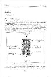
The �nal mesh obtained by the projection method is shown in Figure 6.1, we observe very similar meshes for the other methods. Table 1 lists the
L2 -errors
for
state, adjoint state and control for the di�erent methods. Note that these errors consist of discretization as well as regularization error, where applicable.
3
2.5
2
1.5
1
0.5
0
0
0.5
1
1.5
2
2.5
3
Figure 1. Re�ned mesh to our �rst example. Inner-circle diameter of the mesh is between hmin=0.0102 and hmax=0.0204.
kyh − y ∗ k
kuh − u∗ k
kph − pk
jh (yh , uh )
projection method
1.718e-3
1.558e-2
5.297e-4
8.136e3
moreau-yosida approx.
5.253e-3
2.840e-2
2.840e-5
8.136e3
barrier method
1.687e-4
9.568e-3
9.568e-6
8.136e3
Table 1. Errors in values of
y , u,
and
p
measured in the
L2 -norm,
and
jh .
kuh − u∗ k N=3
N=4
N=5
N=6
projection method
0.6405
0.0975
0.0185
0.0142
moreau-yosida approx.
0.6386
0.0987
0.0301
0.0276
barrier method
0.6416
0.0946
0.0144
0.0035
Table 2. Errors in
u measured in the L2 -norm,
depending on the
number of mesh re�nements.
6.2.
Distributed control with state constraints.
Our second example is taken
from [19], Example 7.2. There is no given analytic solution so we can only compare numerically computed solutions. The problem is given by
min j(y, u) :=
1 κ ky(T )k2L2 (Ω) + kuk2L2 (Q) 2 2 18
subject to
yt − ∆y
= u
∂n y + 10y = 0 y(0) = y0
in
Q,
on
Σ, Ω,
in
and to the state constraint
y ≥ ya := min{−100(t(t − 1) + x(x − 1)) − 49.0, 0.5}
a.e. in
Q.
1
We choose Ω = (0, 1) ⊂ R , T = 1. Further, let y0 = sin(πx) be given and set κ = 10−3 . Obviously, this problem �ts into our general setting with θΩ = 1, θΣ = 0, κQ = κ, κΣ = 0, βQ = 1, βΣ = 0, as well as α = 10. For comparison of the solutions, we use the quadratic programming solver from
2 package to compute a reference solution. Mosek o�ers an interface to
the Mosek
quadprog
Matlab's
function (from the optimization toolbox). For that, we have
to formulate our problem as a discrete optimization problem of the form min
z>
�
� 1 H z + b> z 2
subject to
In contrast to
Aeq z
= beq
Ain z
≤ bin .
quadprog from Matlab's optimization toolbox, MOSEK can handle
sparse matrices so that the limitation of the number of unknowns is lifted.
Results
We compare the solution of all methods with a solution computed by the function
quadprog quadprog
provided by the package MOSEK. Note, that the solution computed by belongs to the unregularized discrete problem formulation, hence mea-
sures do not appear in the optimality system of the problem. In this example, we re�ne the initial grid once. The option all methods. In Table 1 we present the values of
j
hnlin on
is used for
computed by the barrier method,
the projection method, and the Moreau Yosida regularization. For comparison, we give results computed by
quadprog.
In the
quadprog-solver we choose the time λ = 10−3 , γ = 103 , and eps = 10−5 .
step-size as half of the space mesh-size. We set
Barrier method
Projection method
Moreau Yosida regularization
quadprog
jh (yh , uh )
jh (yh , uh )
jh (yh , uh )
jh (yh , uh )
0.0012427
0.0012430
0.0012703
0.0012899
Table 3. Values of jh for the di�erent solution methods.
6.3.
A boundary controlled problem.
Let
Our third example was taken from [3].
Ω = [0, 1] and the time interval I = (0, 5) be given.
The problem formulation
reads as follows: min
2MOSEK
j(y, u) =
κ 1 kyk2L2 (Q) + kuk2L2 (Σ) 2 2
uses an interior point solver.
self-dual algorithm.
It is an implementation of the homogeneous and
For details see the MOSEK manual [16] and the referred literature there.
Incontrast to our approch, MOSEK solves a discrete optimization problem (��rst discretize, then optimize approach�). See the discussion of the di�erent approaches e.g. in [3].
19
subject to
yt − ∆y (21)
=
0
in
Q
y = u y(0) = 0
on
Σ Ω
in
and the point-wise state constraints
ya ≤ y The state constraint is given by
a.e. in
Q.
ya (x, t) = sin(x)(sin(πt/5)) − 0.7,
and
κ
is set to
10−3 . The Dirichlet-boundary condition is di�cult in two ways:
Neither can it be
handled by �nite element methods in the usual way, since the usual technique to substitute the boundary integral of the outer normal derivative of the state by the boundary conditions is not applicable, nor are optimality conditions derived easily, cf. [4]. A possible way to overcome this problem is to approximate the Dirichlet-boundary conditions by Robin boundary conditions: For some replace (21) by
~n · ∇y + αy = αu
on
Σ.
α�1
arbitrarily chosen, we
3 We use Robin boundary conditions for a
correct �nite element implementation of the state equation as well as for a correct implementation of the adjoint equation.
We choose
α = 103 .
In the following,
we assume that there is a continuous optimal state which ensures the existence of optimality conditions wherever we consider an unregularized problem.
Results
There is no analytically given solution for the Betts-Campbell problem, so we can only compare solutions computed by di�erent numerical methods as in the last example.
In the barrier method, we compute a solution for
ν0
on an adaptively
re�ned mesh before we enter the path following loop and twice within the pathfollowing loop. Obviously, the adaption process leads to very small mesh sizes near the boundaries at time bound
ya
t0
and where the distance between the state
is small, i.e. the bound
ya
the grid-adaption process is done in the same call of the function
ngen
y
and the
is almost active. In the projection method,
adaption
with
set to two, that solves the complete problem. Figure 2 shows the adaptively
re�ned meshes. Figure 3 shows the control
u(π, t)
computed by di�erent numerical methods.
In Table 4 we present the values of
j
computed by the barrier method, the
projection method and the Moreau Yosida regularization. For comparison, we give results computed by
quadprog.
Barrier method.
Projection method
Moreau Yosida regularization
quadprog
jh (yh , uh )
jh (yh , uh )
jh (yh , uh )
jh (yh , uh )
0.2327
0.2261
0.2212
0.2346
Table 4. Values of jh for the di�erent solution methods.
7. Conclusion and outlook As shown in [17] for the unconstrained case, IMSEs (here tested Comsol Mul-
tiphysics) can be used also for solving optimal control problems with state constraints. Again, a knowledge about the optimality system for the given problem is
3Some
IMSE like PDETOOL or Comsol Multiphysics use this technique for solving Dirich-
.
let boundary problems by default
In this way it is possible to implement the boundary conditions
directly in Comsol Multiphysics, where it will be corrected internally by using a Robin formulation with a well-chosen parameter
α,
cf. [22].
20
5
5
5
4.5
4.5
4.5
4
4
4
3.5
3.5
3.5
3
3
3
2.5
2.5
2.5
2
2
2
1.5
1.5
1.5
1
1
1
0.5
0.5
0.5
0
0
0.5
1
1.5
2
2.5
0
3
0
1
Figure 2. Adaptive meshes:
2
0
3
0
0.5
1
1.5
2
2.5
3
barrier method (left), projection
method (center), and Moreau Yosida regularization (right). meshes computed by Comsol Multiphysics'
adaption
All
method
with two new grid generations.
0.6 projection quadprog Moreau−Yosida barrier
0.5
0.4
control u
0.3
0.2
0.1
0
−0.1
−0.2
−0.3 0
0.5
1
1.5
2
2.5
3
3.5
4
4.5
5
time t
Figure 3. Solutions of the Betts-Campbell problem.
uh
Controls
computed by the Moreau Yosida regularization (solid line), by
the projection method (dashed), by the MOSEK solver (dash-cross), and by the barrier method (dotted).
quadprog
An analytic
solution is not known. Obviously, the Betts-Campbell problem is symmetric so we show only the control on the boundary with
x = π.
necessary. From the theoretical point of view, the handling of the state constraints and their associated Lagrange multipliers is the most di�cult problem. To guarantee the existence of Lagrange multipliers and to avoid measures in the optimality systems, we apply di�erent regularization techniques in order to justify the use of standard FEM discretizations. To handle (state)-constraints algorithmically, three approaches are considered. Via Lavrentiev-type regularization and source-term representation we arrived at a projection formula for the Lagrange multiplier which leads to an interpretation of the active set strategy as a (semi-smooth) Newton method. The resulting algorithm solved the problem by calls of the solvers
adaption
or
femnlin,
respectively.
Next, we applied a Moreau-Yosida regularization method which can be interpreted as a penalization method and easily implemented with the help of the maximum function. We point out that we used �xed regularization parameters since we do not study the convergence behavior of these methods. It is beyond the scope
21
of this paper to analyze the choice of regularization parameters in more detail. Instead, our main point was to show the implementability of the regularization techniques in IMSEs. At last, we implemented a barrier method by adding a barrier term to the objective functional. The resulting algorithm is a classical (iterative) path following method. Here, in every step a call of a PDE solver is necessary. On the other hand, the regularity of barrier methods permits to pass additional regularization if the order of the rational barrier function is high enough and the solution of the PDEs are su�ciently smooth, cf. [21, Lemma 6.1]. We �rst tested our methods on an example with known exact solution. Then, we applied them to model problems where the solutions are not given. To con�rm our results, we computed reference-solutions by a well-proven program.
All methods
produced similar results in a variety up to ten percent. The di�erence in the results are a combination of discretization and regularization e�ects. Therefore we cannot directly compare the controls de�ned on di�erent grids, but we may expect that a well chosen combination of discretization parameters and parameters inherent to the solution technique such as Lavrentiev parameter, the penalty parameter, or the path parameter in the interior point method, results in a closer approximation of the �real� solution. All together, IMSEs have the capability of solving optimal control problems with inequality constraints and o�er an easily implementable alternative for solving such problems if optimality conditions in PDE formulation are known.
Website WWW.math.tu-berlin.de/Strategies-for-time-dependent-PDE-control.html
References [1] M. Bergounioux, M. Haddou, M. Hintermüller, and K. Kunisch. A comparison of a MoreauYosida-based active set strategy and interior point methods for constrained optimal control problems.
SIAM J. Optimization, 11:495�521, 2000.
[2] M. Bergounioux, K. Ito, and K. Kunisch. Primal-dual strategy for constrained optimal control problems.
SIAM J. Control and Optimization, 37:1176�1194, 1999.
[3] J. T. Betts and S. L. Campbell. Discretize then Optimize. In D. R. Ferguson and T. J. Peters,
Mathematics in Industry: Challenges and Frontiers A Process View: Practice and Theory. SIAM Publications, Philadelphia, 2005. editors,
[4] E. Casas. Pontryagin's principle for state-constrained boundary control problems of semilinear parabolic equations.
SIAM J. Control and Optimization, 35:1297�1327, 1997.
[5] K. Deckelnick and M. Hinze. Convergence of a �nite element approximation to a state constrained elliptic control problem. [6] W. A. Gruver and E. W. Sachs.
SIAM J. Numer. Anal., 45:1937�1953, 2007. Algorithmic Methods in Optimal Control. Pitman, London,
1980. [7] M. Hintermüller, K. Ito, and K. Kunisch. The primal-dual active set strategy as a semismooth Newton method.
SIAM J. Optim., 13:865�888, 2003.
[8] K. Ito and K. Kunisch. Semi-smooth Newton methods for state-constrained optimal control problems.
Systems and Control Letters, 50:221�228, 2003.
[9] K. Krumbiegel and A. Rösch. A virtual control concept for state constrained optimal control
Computational Optimization and Applications. Online �rst. DOI 10.1007/s10589007-9130-0, 2007. Computational Optimization and Applications. problems.
[10] K. Kunisch and A. Rösch. Primal-Dual Active Set Strategy for a General Class of Constrained Optimal Control Problems.
SIAM J. on Optimization, 13:321�334, 2002. Linear and Quasilinear Equa-
[11] O. A. Ladyzhenskaya, V. A. Solonnikov, and N. N. Ural'ceva.
tions of Parabolic Type. American Math. Society, Providence, R.I., 1968. Optimal Control of Systems Governed by Partial Di�erential Equations. Springer-
[12] J. L. Lions.
Verlag, Berlin, 1971. [13] C. Meyer, U. Prüfert, and F. Tröltzsch. On two numerical methods for state-constrained elliptic control problems.
Optimization Methods and Software, 22(6):871�899, 2007.
[14] C. Meyer, A. Rösch, and F. Tröltzsch. Optimal control of PDEs with regularized pointwise state constraints.
Computational Optimization and Applications, 33:209�228, 2006. 22
[15] C. Meyer and F. Tröltzsch. On an elliptic optimal control problem with pointwise mixed
[16]
control-state constraints. In A. Seeger, editor, Recent Advances in Optimization. Proceedings of the 12th French-German-Spanish Conference on Optimization held in Avignon, September 20-24, 2004, Lectures Notes in Economics and Mathematical Systems. Springer-Verlag, 2005. MOSEK ApS. The MOSEK optimization tools manual. Version 5.0 (Revision 60). http://www.mosek.com, 2007.
[17] I. Neitzel, U. Prüfert, and T. Slawig. Strategies for time-dependent PDE control using an integrated modeling and simulation environment. part one: problems without inequality constraints. Technical Report 408, Matheon, Berlin, 2007. [18] I. Neitzel and F. Tröltzsch. On regularization methods for the numerical solution of parabolic control problems with pointwise state constraints. Technical report, SPP 1253, 2007. to appear in ESAIM: COCV. [19] U. Prüfert and F. Tröltzsch. An interior point method for a parabolic optimal control problem with regularized pointwise state constraints.
ZAMM, 87(8�9):564�589, 2007.
[20] J.-P. Raymond and H. Zidani. Pontryagin's principle for state-constrained control problems governed by parabolic equations with unbounded controls.
tion, 36:1853�1879, 1998.
SIAM J. Control and Optimiza-
[21] A. Schiela. Barrier Methods for Optimal Control Problems with State Constraints. ZIBReport 07-07, Konrad-Zuse-Zentrum für Informationstechnik Berlin, 2007. [22] The MathWorks.
Partial Di�erential Equation Toolbox User's Guide. The Math Works Inc.,
1995.
Optimale Steuerung partieller Di�erentialgleichungen. Theorie, Verfahren und Anwendungen. Vieweg, Wiesbaden, 2005.
[23] F. Tröltzsch.
[24] F. Tröltzsch and I. Yousept. A regularization method for the numerical solution of elliptic
boundary control problems with pointwise state constraints. Computational Optimization and Applications. Online �rst. DOI 10.1007/s10589-007-9114-0, 2008.
[25] M. Ulbrich and S. Ulbrich. Primal-dual interior point methods for PDE-constrained optimization. [26] J. Wloka.
Mathematical Programming. Online �rst.DOI 10.1007/s10107-007-0168-7, 2007. Partielle Di�erentialgleichungen. Teubner-Verlag, Leipzig, 1982.
Address: Ira Neitzel, Uwe Prüfert: TU Berlin - Fakultät II, Institut für Mathematik, Straÿe des 17. Juni 136, 10623 Berlin, Germany. Thomas Slawig: ChristianAlbrechts-Universität zu Kiel, Technische Fakultät, Christian-Albrechts-Platz 4, 24118 Kiel, Germany
23