The area of the lobes of the resultant turnstile is given asymptotically by "exp(- 2=h)"(h), where "(h) is an even Gevrey-1 function such that "(0) /= 0 and the radius.
Singular separatrix splitting and the Melnikov method: An experimental study Amadeu Delshams and Rafael Ram��rez-Ros Departament de Matem�atica Aplicada I Universitat Polit�ecnica de Catalunya Diagonal 647, 08028 Barcelona, Spain Abstract
We consider families of analytic area-preserving maps depending on two parameters: the perturbation strength " and the characteristic exponent h of the origin. For " = 0, these maps are integrable with a separatrix to the origin, whereas they asymptote to �ows with homoclinic connections as h ! 0+ . For �xed " 6= 0 and small h, we show that these connections break up. The area of the lobes of the resultant turnstile is given asymptotically by " exp(;�2 =h)�" (h), where �"(h) is an even Gevrey-1 function such that �"(0) 6= 0 and the radius of convergence of its Borel transform is 2�2 . As " ! 0, the function �" tends to an entire function �0 . This function �0 agrees with the one provided by the Melnikov theory, which cannot be applied directly, due to the exponentially small size of the lobe area with respect to h. These results are supported by detailed numerical computations� we use an expensive multiple-precision arithmetic and expand the local invariant curves up to very high order.
Keywords: Area-preserving map, singular separatrix splitting, Melnikov method, numerical experiments AMS Subject Classi�cation (1991): 34C37,34E05,34E15,65L12
1 Introduction The problem
In this paper, we consider the following family of planar standard-like maps
F (x� y) = (y� ;x + U (y))� 0
U (y) = �0 log(1 + y2) + "V (y)� 1
Singular splitting and the Melnikov method 2 where V (y) = Pn 1 Vny2n is an even entire function. Provided that �0 + V1" > 1, the origin O = (0� 0) is a hyperbolic �xed point with Spec� dF (O)] = fexp(�h)g, and its characteristic exponent h > 0 is given by �
cosh h = �0 + V1": Moreover, when " vanishes, F becomes integrable with a separatrix to the origin. Thus, the map F can be considered as a perturbation of an integrable map, " being the perturbation strength. These two parameters, h > 0 and ", will be considered the intrinsic parameters of the map F under study. Our goal is to show that for " 6= 0 and for a general perturbation, the separatrix splits and exactly two (transverse) primary homoclinic points, z+ and z , appear on the quadrant fx� y > 0g. By primary homoclinic orbits we mean that these orbits persist for all " small enough. The pieces of the perturbed invariant curves between the points z enclose a region called lobe. Our measure of the splitting size will be the area A of this lobe, see �gure 2. This lobe area is a homoclinic symplectic invariant, that is, it does not depend on the symplectic coordinates used, and all the lobes have the same area. Lobe areas also measure the �ux along the homoclinic tangle, which is related to the study of transport �MMP84, MMP87, Mei92]. Both parameters, h > 0 and ", will be small \enough", but the exact interpretation of this sentence is crucial for understanding the di�erent kinds of results to be presented. Speci�cally, we are going to deal with the following situations: 1. The regular case: �xed h > 0, and " ! 0. 2. The singular case: h ! 0+. In its turn this case subdivides in two sub-cases: (a) The non-perturbative case: " �xed and h ! 0+. (b) The perturbative case: " = o(hp) and h ! 0+, for some p � 0. Both analytical and numerical results for the splitting of separatrices are obtained. The analytical results are expressed in terms of the Melnikov potential of the problem, which gives explicit formulae for our map. This is the reason for our choice of the map above as a model for this paper, instead of more celebrated maps like the H�enon map or the standard map. The name \singular" for the case h ! 0+, is due to the fact that the lobe areas are exponentially small in h. The measure of such small quantities requires a very careful treatment, both from a numerical and an analytical point of view. ;
�
Outline of results
In the regular case, for 0 < j"j < " (h) = o(exp(;�2 =h)), the discrete version of the usual Melnikov method �DR96, DR97b] ensures the existence of two transverse, primary homoclinic orbits, and provides the �rst order approximation, in the perturbation �
Singular splitting and the Melnikov method strength ", of the lobe area:
A = "AMel + O("2)�
AMel = e
3 �2 =h
;
h
i �0(h) + O(e 2�2 =h) � ;
where �0(h) = Pn 0 �0nh2n is an even entire function. If V (y) is a polynomial, �0(h) can be explicitly computed in a �nite number of steps. For instance, �0 (h) = 8�2 2 h 2 for V (y) = y, and �0(h) = 38 �2 4 h 2�1 + �2h 2 ] for V (y) = y3. The non-polynomial case is harder, although some P closed formulae can be obtained. In particular, �0(0) = �00 = 8�Vb (2�), where Vb ( ) = n 1 Vn 2n 1=(2n ; 1)! is the Borel transform of V (y). In the singular case, the result above cannot be applied, since it requires " to be exponentially small in h. There are, however, a couple of analytical results that hold. In the non-perturbative case, under the assumption �
;
;
0
;
0
;
�
(V1 + 2V2)" < 1� there exist homoclinic orbits for h > 0 small enough, and an exponentially small in h > 0 upper bound is provided for the lobe area. In the perturbative case " = o(hp), with p > 6, under the assumption Vb (2�) 6= 0, the existence of two transverse, primary homoclinic orbits in the �rst quadrant is proved, and an asymptotic expression for the area lobe is given:
A = "e
;
�2 =h
h
i
8�Vb (2�) + O(h2)
(h ! 0+):
Most of these analytical results are spread out over several recent papers of the authors �DR96, DR97b, DR97a]. For the convenience of the reader, we have collected in the present paper the main ideas. The heart of this paper is dedicated to study numerically the situations not covered by the analytical results for the singular case. The numerical experiments have been performed for the simplest even perturbed potentials, that is, for the linear perturbation "V (y) = "y, and the cubic one "V (y) = "y3. In the non-perturbative case, the following asymptotic expansion for the lobe area A is numerically established 0
0
A � "e
�2 =h X �" h2n n n 0
;
(h ! 0+� " �xed):
�
The sign � means that the series Pn 0 �"nh2n is an asymptote, that is, if one retains a �nite number of the �rst successive terms, the error has the order of the �rst missing term: � � N � � 2 =h X � � � " 2 n 2N +2 e �2 =h ): �A ; " e � h � = O("h n � � �
;
The coe�cients
�"n
;
n=0
are real numbers such that
h i �"n = (2n)!(2�2) 2n(2n)4 �" + O(n 1) ;
;
1
(n ! +1)�
Singular splitting and the Melnikov method 4 for some non-zero constant �"P. In particular, Pn �"nh2n is divergent for all h 6= 0, but its Borel transform �c"(h) = n �"n 2n 1=(2n ; 1)! is convergent for j j < 2�2. This implies that the function �"(h) �P" 1 exp (�2=h) A is Gevrey-1 of type � = 1=2�2. Let us recall that a function f (x) � n 0 fnxn is said to be Gevrey-r of type � if there are positive constants C� > 0 such that jfnj � C�rn;(rn + ), where ;(z) stands for the Gamma function. (We follow the notations of �RS96].) In the perturbative case, we study the behavior of the objects �"(h), �"n, �" , checking that all of them tend to well-de�ned limits, as " ! 0. (That is, for " = o(1). In the notation " = o(hp), this means that p = 0.) First, the function �"(h) tends to the Melnikov prediction �0(h) when the perturbation strength " tends to zero more precisely, 1
;
;
�
1
uniformly in h 2 (0� 1]:
�"(h) = �0 (h) + O(")�
The coe�cients �"n of the Gevrey series for �"(h) also converge to the Taylor coe�cients �0n of the entire function �0 (h). ( For example, �"0 = 8�Vb (2�)+O(").) Obviously, this convergence cannot be uniform in the index n, since lim j�"nj = n + !
1
(
0 if " = 0 +1 otherwise.
Finally, lim" 0 �" = 0, since �" quanti�es the growth of the coe�cients �"n, and �0n = lim" 0 �"n gives a decreasing sequence. In fact, one has !
1
1
!
�"
1
= "�0
1
+ O("2)�
where
�0
12� 4 if V (y) = y : = ; ;16=3 if V (y) = y3 (
1
;
0 0
Relation to other work By now, there is a well-developed literature on singular perturbations for maps. Results showing that the splitting size is exponentially small in the characteristic exponent h have been obtained by many authors. For the sake of brevity, we review results concerning analytic area-preserving maps, both from a theoretical and a numerical point of view. For a review of the results concerning �ows, we refer to �DS97, DRS98], and the references therein. The �rst relevant results are exponentially small upper bounds of the splitting size for analytic area-preserving maps with a weakly hyperbolic �xed point and homoclinic points to it �Nei84, FS90, Fon95, FS96, Gel96]. Roughly speaking, in these papers it is proved that the maps asymptote to a Hamiltonian �ow with a separatrix when the characteristic exponent h tends to zero. Then, the splitting size is O (exp(; =h)), for any positive constant smaller than 2�d, d being the analyticity width of the separatrix of the limit �ow. No more general results are known. In order to compare this result with the next ones, it is convenient to formulate it as splitting size = e
;
�=h �(h)�
�(h) bounded when h ! 0+:
(1.1)
Singular splitting and the Melnikov method 5 The next step was the attainment of exponentially small asymptotic formulae in some standard-like maps, by V. Lazutkin and co-workers �Laz84, LST89, GLT91], see also �HM93, Sur94, Tre96]. For instance, regarding the standard map and the H�enon map, in these works it is claimed that the splitting has an asymptotic behavior of the form !0 h� exp(; =h), for some constants !0 6= 0, > 0, and , that is, splitting size = h� e
�=h �(h)�
;
�(h) continuous at h = 0 and �(0) 6= 0:
(1.2)
The constant !0 = �(0) is de�ned by means of a nonlinear parameterless problem which only can be solved numerically, is obtained by linearization about the separatrix in the complex plane, and = 2�d, where d is again the analyticity width of the unperturbed separatrix. A complete proof of these asymptotic formulae has not been published yet, but there is little doubt about its validity. It should be noted that there exist examples where a formula like (1.2) cannot hold, because the splitting behaves asymptotically like !0h� exp(; =h) cos( =h) with 6= 0, see �GLT91, SMH91]. The maps here considered do not fall into this class. The strongest analytical results on the regularity of the function �(h) were contained in �GLS94, Che95, Nik95], where it is stated (again without proofs) that splitting size = h� e
�=h �(h)�
;
�(h) smooth at h = 0 and �(0) 6= 0�
(1.3)
for the standard map �GLS94], the H�enon map �Che95], and the twist map �Nik95]. All these works contains formulae like
!�O] � h� e
�=h X ! h2n � n n 0
;
�
where !�O] stands for the Lazutkin's homoclinic invariant introduced in �GLT91] for some distinguished symmetric homoclinic orbit O. Only a few coe�cients !n were explicitly computed in these works: the �rst �ve coe�cients in �GLS94], the �rst three in �Nik95] and just two in �Che95]. Then, a natural question appears: Which is the growth rate of the coe�cients !n when n ! +1? Or equivalently, is �(h) somewhat stronger than smooth? A numerical answer involves the computation of many of such coe�cients. Recent numerical experiments performed by C. Sim�o suggest that the asymptotic series P 2n n 0 !n h are divergent, although their Borel transforms are convergent, that is, �
splitting size = h� e
�=h �(h)�
;
�(h) Gevrey-1 at h = 0 and �(0) 6= 0:
(1.4)
Our numerical results fall just into this class, with the area A as our measure of the splitting size, and the coe�cients �"n playing the r^ole of !n. The computation of !n for relatively large values of n (namely, up to n = 100), requires the use of an expensive multiple-precision arithmetic, so that these experiments are on the edge of the current computer possibilities. Therefore, further numerical results improving these ones are unlikely to appear in a near future.
Singular splitting and the Melnikov method 6 Regarding rigorous results, to the best of our knowledge, the paper �DR97a] is the only place where a behavior like (1.2) has been rigorously proved for some areapreserving maps. This makes evident that experimental studies are much more advanced than analytical ones. However, numerical results of the form (1.4) open the door to new techniques, like resurgence tools, that have been already applied to the rapidly forced pendulum �Sau95], and may be successful to �ll this gap between analytical and numerical results.
Outline of the computations The area of the lobes of the turnstile created when the separatrices split is computed using the MacKay-Meiss-Percival action principle �MMP84, Eas91], in which the lobe area is interpreted as a di�erence of actions. The numerical computation of such exponentially small lobe areas with arbitrary precision forces us to:
use an expensive multiple-precision arithmetic,
expand the invariant curves up to an optimal order, which is very large,
take the greatest advantage of symmetries and/or reversors. Clearly, the �rst item is unavoidable, due to the strong cancellation produced when subtracting the (exponentially close) actions, and also due to the requirement of arbitrary precision in the �nal result. The second item is intended to take the initial iterates far enough of the weakly hyperbolic point so that the homoclinic points z can be attained in (relatively) few iterations: we are able to �nd the (optimal) order which minimizes the computer time. This optimal choice of order avoids an undesirable accumulation of rounding errors due to the large number of operations. Finally, the third item is crucial to overcome certain stability problems. Those algorithms for computing homoclinic points that do not take into account symmetries and/or reversors (if they exist, of course) have condition numbers inversely proportional to the splitting size, see for instance �BK97, pag. 1218]. Therefore, they would be exponentially ill-conditioned for our singular maps! We have improved the methods used in �LM96] to compute lobe areas. In that paper a similar problem was studied, but the invariant curves were developed only to �rst (linear) order and a standard double-precision arithmetic was used. Due to this, the computations in �LM96] only gave accurate results for lobe areas A � 10 14, that is, for characteristic exponents h not smaller than 1=3. In this work, we have been able to compute lobe areas less than 10 4200 (that is, we have arrived up to h = 0:001), with a relative error less than 10 900. The computation for such extreme cases takes between two and three days on a Pentium 200 under a Linux operative system, depending on the potential V (y). More than 5200 decimal digits in the arithmetic and 1300 coe�cients in the Taylor expansion of the invariant curves have been needed for these accurate computations. �
;
;
;
Singular splitting and the Melnikov method 7 So far, and to the best of our knowledge, the most re�ned (published) experiments about singular splittings for maps were those of �FS90], where splittings of order 10 200 were numerically computed following the above-mentioned items. Other experiments with multiple-precision arithmetic are contained in �FS96], but only order one (that is, linear) expansions of the invariant curves were used in that paper. In �BO93] a quadruple-precision together with high order expansion were used to study the rapidly forced pendulum. ;
Outline of the paper The rest of the paper is devoted to explain how our results have been obtained. In the next section, the model is introduced. In section 3, the regular case " ! 0 and h �xed is discussed. We review how to compute the O(")-approximation of the lobe area using the discrete version of the Melnikov method. In particular, the entire function �0(h) is introduced. Section 4 is devoted to the singular limit h ! 0+. The asymptotic behavior of �"(h) is studied and the connection with the Melnikov theory is drawn. The results in this section are the heart of the paper. In section 5, the algorithm used to compute lobe areas with an arbitrary accuracy is described. This is the key tool in this work. The numerical calculations are complicated by problems of stability, precision and computer time, so we provide su�cient detail to show how these problems can be overcome. Finally, further numerical experiments related to singular separatrix splittings for maps are proposed in section 6. They will be the subject of future research.
2 The model The family of standard-like maps under study is given by F (x� y) = (y� ;x + U (y))� U (y) = �0 log(1 + y2) + "V (y)� (2.1) where V (y) = Pn 1 Vny2n is an even entire function. For � := �0 + "V1 > 1� n o the origin O = (0� 0) is a hyperbolic �xed point with Spec� dF (O)] = e h , where the characteristic exponent h > 0 is determined by cosh h = �. We will consider the characteristic exponent h and the perturbation strength " as the intrinsic parameters of our model. Accordingly, for every h > 0 and every real ", we rewrite the map (2.1) in the form 0
�
�
F (x� y) = (y� ;x + U (y))� U (y) = U0 (y) + "U1(y)� U0 (y) = � log(1 + y2)� U1 (y) = V (y) ; V1 log(1 + y2): 0
(2.2)
From now on, the subscript \0" will denote an unperturbed quantity, that is, " = 0, and the following notations will be used without further comment: � = cosh h� = sinh h� � = eh : (2.3)
Singular splitting and the Melnikov method
8
C+
C0
;
Figure 1: The zero level of I0 for h = 2.
The unperturbed model
Setting " = 0 in (2.2), we obtain the so-called McMillan map �McM71] � ! 2 �y F0 (x� y) = (y� ;x + U0(y)) = y� ;x + 1 + y2 � which is an integrable exact map, with a polynomial �rst integral given by I0 (x� y) = x2 ; 2�xy + y2 + x2 y2: The phase space associated to F0 is rather simple, since it is foliated by the level curves of the �rst integral I0, which are symmetric with respect to the origin. As � > 1, the zero level of I0 is a lemniscate, whose loops are separatrices to the origin (see �gure 1). From now on, we will concentrate on the separatrix $ in the quadrant fx� y > 0g, which can be parameterized by z0(t) = (x0(t)� y0(t)) = ( 0(t ; h=2)� 0(t + h=2))� 0(t) = sech t: (2.4) This parameterization is called natural since F0 (z0(t)) = z0 (t + h), a fact that can be checked simply by noting that 0(t) is a homoclinic solution of the di�erence equation
0(t + h) + 0(t ; h) = U0 ( 0(t)): (2.5) 0
0
Singular splitting and the Melnikov method
9
C+
Wu z+
A
C z
;
;
Ws
Figure 2: The homoclinic points z and the lobe area A for "V (y) = y3=40 and h = 2. �
0
A natural parameterization is unique except for a translation in the independent variable. To determine it, it is worth looking at the reversors of the map. Indeed, the involution R+(x� y) := (y� x) is a reversor of the McMillan map F0 , that is, F0 1 = R+ F0 R+. The separatrix $ is R+-symmetric, i.e., R+$ = $, and intersects transversely the �xed set C + := fz : R+z = zg of R+ in one point z0+. The parameterization (2.4) of $ has been chosen to satisfy z0 (0) = z0+. Moreover, the involution R0 := F0 R+ is another reversor of F0 . The separatrix $ is also R0 -symmetric and intersects transversely the �xed set C0 of R0 in one point z0 , and it turns out that z0 (h=2) = z0 . The associated orbits O0+ := fz0(nh) : n 2 Zg, O0 := fz0 (h=2 + nh) : n 2 Zg, are called symmetric homoclinic orbits, since R+O0+ = O0+, R0 O0 = O0 . ;
;
;
;
;
;
;
;
;
;
;
The perturbed model For " = 6 0, the phase portrait of the exact map (2.2) looks more intricate. The origin is
a hyperbolic �xed point with the same characteristic exponent h, since the perturbation "U1(y) = O(y3) does not contain linear terms at the origin. We denote by W u�s its unstable and stable invariant curves with respect to F . Since the map (2.2) is odd, the 0
Singular splitting and the Melnikov method 10 invariant curves are symmetric with respect to the origin, so that we concentrate only on the positive quadrant fx� y > 0g. By the form of the perturbation, R+ is also a reversor of F , as well as the involution R := F R+ , which is given by R (x� y) = (x� ;y + U (x)). Their �xed sets C = fz : R z = zg are important because R (W u ) = W s. Consequently, any point in the intersection C \ W u is a homoclinic point (see �gure 2), and gives rise to a symmetric homoclinic orbit. Since the separatrix $ intersects transversely the unperturbed curve C0 at the point z0 , there exists a point z = z0 + O(") 2 C \ W u and, therefore, there exist at least two symmetric homoclinic orbits on the quadrant fx� y > 0g, for j"j small enough. They are called primary since they exist for arbitrary small j"j. ;
;
�
0
�
�
�
�
�
�
�
�
3 The regular case Along this section, the characteristic exponent h > 0 will be considered �xed, and then " ! 0. In particular, any sentence like \for j"j small enough" will mean: \there exists " (h) > 0 such that for j"j < " (h)". Typically, " (h) will be exponentially small in h. �
�
�
3.1 The Melnikov theory for exact planar maps
We now recall some perturbative results to detect the existence of transverse homoclinic orbits for exact maps. For simplicity, we will assume that all the objects are smooth and we shall restrict the discussion to maps on the plane with the usual symplectic structure: the area. Given the symplectic form ! = dx ^ dy = d(;y dx) on the plane R 2 , a map F : R 2 ! R 2 is called exact if there exists some function S : R 2 ! R such that F (y dx) ; y dx = dS . The function S is called the generating function of F and, except for an additive constant, it is uniquely determined. Let F0 : R 2 ! R 2 be an integrable exact di�eomorphism with a separatrix $ to a hyperbolic �xed point z0 . Next, consider a family of exact di�eomorphisms F" = F0 + "F1 +O("2), as a general perturbation of the situation above, and let S" = S0 +"S1+O("2) be the generating function of F". We introduce the Melnikov potential of the problem as the smooth real-valued function L : $ ! R given by X L(z) = Sb1(zn )� zn = F0n(z)� z 2 $� (3.1) �
1
n Z 2
where Sb1 : R 2 ! R is de�ned by Sb1 = S1 ; y dx(F0 )�F1]. (In components, writing F0 = (X0� Y0), F1 = (X1� Y1), Sb1 is simply given by Sb1 = S1 ; Y0X1.) In order to get an absolutely convergent series (3.1), Sb1 is determined by imposing Sb1 (z0 ) = 0. The di�erential of L is a geometrical object which gives the O(")-distance between the perturbed invariant curves W"u�s. More precisely, let (t� e) be some cotangent coordinates adapted to $|that is, in these coordinates the separatrix $ is given locally by 1
Singular splitting and the Melnikov method 11 fe = 0g and the symplectic form ! reads as dt ^ de|and let fe = E"u�s(t)g be a part of W"u�s . (Let us recall that cotangent coordinates can be de�ned in neighborhoods of Lagrangian sub-manifolds �Wei73].) Then, in �DR97b] it is shown that
E"u (t) ; E"s(t) = "L (t) + O("2)� 0
and that the construction above does not depend on the cotangent coordinates used. The following theorem �DR97b, Theorem 2.1] is a straightforward corollary of this geometric construction.
Theorem 3.1 Under the above notations and hypotheses, the non-degenerate critical
points of L are associated to perturbed transverse homoclinic orbits. Moreover, when all the critical points of L are non-degenerate, all the primary homoclinic orbits arising from $ are found in this way. Finally, if z and z are consecutive (in the internal order of the separatrix) non-degenerate critical points of L, their associated perturbed homoclinic orbits determine a lobe with area 0
A = "�L(z) ; L(z )] + O("2): 0
3.2 The regular analytical result
We are now ready to apply the theory above to our model. It is worth noting that the knowledge of the natural parameterization (2.4) of the unperturbed separatrix $ will be the crucial point to compute explicitly the Melnikov potential (3.1). The map F = F0 + "F1 + O("2) given in (2.2) is exact with generating function S (x� y) = ;xy + U0 (y) + "U1 (y). Writing its expression in components F0 = (X0� Y0), F1 = (X1� Y1), it turns out that X1 = 0, and consequently Sb1 (x� y) = S1 (x� y) = U1 (y). The parameterization (2.4) allows us to write the Melnikov potential (3.1) of our problem as
L(t) := L(z0 (t)) =
X
n Z
U1(y0(t + hn)) =
2
X
�f (t + hn) ; g(t + hn)]�
n Z 2
where f (t) := V ( 0(t + h=2)) and g(t) := V1 log (1 + 0(t + h=2)2). We are now confronted to the computation of a series for L(t), which is a doublyperiodic function: L(t) = L(t + h) = L(t + � i). Consequently, the explicit computation of L(t) can be performed through the study of its singularities for complex values of the discrete time t �DR96]. P For example, Lg (t) := n g(t + hn) is easily computed simply by noting that Lg (t) has no singularities and, therefore, it must be constant by Liouville's theorem. The exact value of the constant is not important for our purposes, since the intrinsic geometrical object associated to the problem P is L (t) rather than L(t). The computation of Lf (t) := n f (t + hn) follows the same lines, although is more complicated. We sketch here the main ideas, and refer to �DR97a] for the details. 0
Singular splitting and the Melnikov method 12 First, we notice that the singularities of f (t) are just located on the set ;h=2 + P � i =2 + � i Z. Next, we denote by n Z vn(h)� 2n the Laurent expansion around � = 0 of the function � 7! f (;h=2 + � i =2 ; i h� ), and note that v n(h) are even entire functions such that v n(0) = Vn, for all n � 1. Finally, we introduce the even entire function 2
;
;
X (2� )2n 1 0 � (h) := 8� (2n ; 1)! v n(h) = 8�Vb (2�) + O(h2)� n 1 ;
(3.2)
;
�
where Vb ( ) := Pn 1 Vn 2n 1=(2n ; 1)! is the so-called Borel transform of V (y). Then, the following asymptotic formula holds for the Melnikov potential L = Lf ; Lg = Lf (modulo an additive constant): ;
�
L(t) = e
;
�2 =h cos(2�t=h)
h
;�0(h)=2 + O(e
i
2�2 =h )
;
:
(3.3)
If V (y) is a polynomial, �0(h) can be explicitly computed in a �nite number of steps �DR96]. For instance, for the perturbations used in the numerical experiments, 2 2 2 for V (y) = y : �0(h) = 88��2 4hh 2�1 + �2h 2 ] for V (y) = y3 3 (
;
0
;
;
(3.4)
0
From the formula (3.2), it is clear that if Vb (2�) 6= 0 and h is small enough, the set of critical points of the Melnikov potential (3.3) is hZ=2. All of them are non-degenerate, and parameterize the two unperturbed, symmetric, primary homoclinic orbits O0 . Now, the following result is a corollary of theorem 3.1. �
Theorem 3.2 Assume that V (2�) 6= 0. Then, for any small enough (but �xed) charb
acteristic exponent h > 0, there exists a positive constant " = " (h) such that the map (2.2) has exactly two transverse, symmetric, primary homoclinic orbits O in the quadrant fx� y > 0g, for 0 < j"j < " . These orbits determine a lobe with area A = "AMel + O("2), where the �rst order in " approximation AMel is given by �
�
�
�
AMel = L(h=2) ; L(0) = e
;
�2 =h
h
i �0 (h) + O(e 2�2 =h) : ;
(3.5)
Remark 3.1 We note that "AMel is the dominant term for the Melnikov formula of the lobe area A only if j"j < " (h) = o(exp(;�2 =h)). Otherwise, in the case " = O(hp), the �
Melnikov theory as described is not useful, since it only gives the very coarse estimate A = O(h2p), and not the desired exponentially small asymptotic behavior.
4 The singular case
Along this section, h ! 0+, and we will study analytically and numerically two di�erent situations for the parameter ":
The non-perturbative case: " �xed and h ! 0+.
Singular splitting and the Melnikov method 13
The perturbative case: " = o(hp) and h ! 0+, for some p � 0. For the analytical results we only assume that the perturbed potential V (y) is an even entire function. The numerical experiments have been performed for the simplest even perturbed potentials, that is, for the linear perturbation "V (y) = "y, and the cubic one "V (y) = "y3. 0
0
4.1 Singular analytical results
The non-perturbative case The limit h ! 0+ in (2.2) is highly singular, since all the interesting dynamics is contained in a O(h) neighborhood of the origin, which becomes a parabolic point of the map for h = 0. To see clearly this behavior, we perform the following linear change of variables:
z = Cw�
1=2 1=2 C = h ��1=2 �� 1=2 � �
!
;
;
z = (x� y)�
w = (u� v)�
that is, we diagonalize the linear part of (2.2) at the origin and we scale by a factor h. Then, � � C 1 F C w = w + hX 0(w) + O(h2)� (4.1) where � � X 0(u� v) = u ; �(u + v)3 � ;v + �(u + v)3 � � = 1 ; (V1 + 2V2)"� (4.2) is a Hamiltonian vector �eld, with associated Hamiltonian H 0(u� v) = uv ; �(u + v)4=4: (4.3) Expression (4.1) shows clearly that F is O(h)-close to the identity, and that, after the change of variables z = Cw, the map (2.2) asymptotes to the Hamiltonian �ow associated to the vector �eld (4.2) when h ! 0+. When such situation takes place, it is known �Fon89] that the map (2.2) will have homoclinic points to the origin for any small enough h, if and only if the limit Hamiltonian �ow has a homoclinic orbit to the origin. From the expression (4.3), we see that the zero level fH 0(u� v) = 0g contains homoclinic connections to the origin if and only if � > 0, i.e., if (V1 + 2V2)" < 1: (4.4) Assuming � > 0, the homoclinic orbit of the Hamiltonian (4.3) is given by � ! cosh t ; sinh t cosh t + sinh t 0 1 = 2 � 2 cosh2 t � w (t) = � 2 cosh2 t which is analytic on the strip ft 2 C : j=tj < d := �=2g. In this situation, it is also well-known �FS90] that the splitting size is O(exp(; =h)), for all < 2�d = �2. We summarize these �rst analytical results. ;
;
Singular splitting and the Melnikov method 14 Theorem 4.1 For any real " verifying (4.4), and any 2 (0� �2), there exists N = N ("� ) > 0 such that the area of the lobe between the invariant curves of the map (2.2) satis�es: jAj � N e �=h (" �xed� h ! 0+): ;
The perturbative case The previous theorem gives only an upper bound for the lobe area and not an asymptotic one (the constant N ("� ) can blow up when ! �2). In particular, it does not exclude the case A = 0, that is, it cannot detect e�ective splitting of separatrices. In the perturbative case " = o(hp), for p > 6, the following theorem gives an asymptotic expression for the lobe area in terms of the Melnikov potential, and establishes transversal splitting of separatrices. The version presented here is slightly more general than the one contained in �DR97a], since we have dropped out the hypothesis V (0) = 2V1 = 0 of that paper. 0
Theorem 4.2 Assume that " = o(hp), p > 6. Then, if V (2�) 6= 0, there exists h > 0 b
�
such that the map (2.2) has exactly two transverse, symmetric, primary homoclinic orbits in the �rst quadrant, for all 0 < h < h . Moreover, they enclose a lobe with area �
A = "e
�2 =h
;
h
i
8�Vb (2�) + O(h2)
(h ! 0+):
If Vb (2� ) = 0,2 there may exist more primary homoclinic orbits, but the area of any lobe is O("h2 e � =h). ;
Proof. For V1 = 0, the result above is just the Main Theorem of �DR97a]. For V1 6= 0, the perturbative potential U1 (y) = V (y) ; V1 log(1 + y2) in (2.2) is not longer an entire function, due to the term g(y) := V1 log(1 + y2), and the Main Theorem of �DR97a] cannot be applied directly. However, this result follows from the following observations: 1. As we have already seen in section 3.2, the Melnikov potential L(t) is not a�ected by the contribution of Lg (t). 2. One can easily bound g ( 0(t) + �) in such a way that the estimates of Lemma 3.5 in �DR97a] do not change. Now, the rest of arguments in �DR97a] remain applicable, and the result follows. 2 We �nish this account of analytical results by remarking that, to the best of our knowledge, the result above, jointly with �DR97a], are the �rst analytical results about asymptotics for singular separatrix splitting for a map with a complete and rigorous proof. 0
Singular splitting and the Melnikov method
15
4.2 Singular numerical results
In the regular case, we dispose of formula (3.5) for the lobe area A, in terms of an even analytic function �0 (h), with a fairly simple expression (3.4) for V (y) = y� y3. These regular results suggest that in the singular case, for every �xed " verifying (4.4), the actual formula for the lobe area may have the form 0
A = "e
�2 =h
;
h
i �"(h) + O(e 2�2 =h) � ;
(�xed "� h ! 0+)�
(4.5)
for a function �"(h) given by an asymptotic series of the form �"(h) �
X
n 0
�"nh2n�
(�xed "� h ! 0+):
(4.6)
�
The sign � means that the series Pn 0 �"nh2n needs not to be convergent, but only asymptotic, that is, if one retains a �nite number of the �rst successive terms, the error has the order of the �rst missing term: �
� N � X " " 2 n � (h) ; �nh ��� = O(h2N +2 ): n=0
� � � � �
We are interested in computing a relevant number of the coe�cients �"n for some signi�cant perturbations "V (y), in such a way that we can measure their asymptotic behavior, and describe the analytical properties of the function �"(h). To such end, once we have chosen a perturbation "V (y), we compute the lobe area A with a relative error less than �, for a net N of values of the characteristic exponent h. We take an equidistant net in h2, due to the fact that we expect that the asymptotic series (4.6) will contain only even powers of h. That is, we take 0
0
N = fhj := j 1=2 � : j = 1� : : : � ` + 1g for some (relatively) small positive number � and some (relatively) large natural `. We have chosen the values
� = 10
900 �
;
� = 0:001�
` = 99:
(4.7)
Other choices are also possible, but, taking into account our purposes, it is not worth taking values of � much smaller than exp (;2�2 =h`+1). Let us explain this. We do not know how to compute directly the function �"(h), but only how to approximate it by " 1 exp (�2 =h) A. Once obtained the approximated values of �"(h) on the net N , they will be the input of some algorithm which computes the �rst ` + 1 asymptotic coe�cients �"n. This explains why it is rather absurd to take � too small, being � � exp (;2�2 =h) the greatest accuracy we can expect on approximating �"(h) by " 1 exp (�2=h) A. Since all the values in the net are computed with the same accuracy, we must take � not much smaller than exp (;2�2=h`+1) = max1 j `+1 exp (;2�2 =hj ). ;
;
��
Singular splitting and the Melnikov method
16
Figure 3: �"n vs. n, for " = 0:1. The dashed lines correspond to the limit value �" , which is found by extrapolation. Left: V (y) = y and �" = ;9:7737740885 : : : � 10 3. Right: V (y) = y3 and �" = ;4:6302913918 : : : � 10 1. 0
1
;
1
0
;
1
An interpolation method based on Neville's algorithm has been used to compute the asymptotic coe�cients of �"(h) from the values on the net N . That is, we compute the P` " polynomial P (h) = n=0 Pn"h2n which interpolates �"(h) on N , and next we approximate �"n by Pn", for n = 0� : : : � `. Although equidistant interpolation using polynomials of high degree (in our case, degree ` in h2 ) is in some cases an ill-conditioned problem, we have checked that the coe�cients �"n so obtained are accurate enough for our purposes. Concretely, with the choice (4.7), this method gives at least 860 ; 9n signi�cant decimals digits for �"n, n = 0� : : : � 95. (The accuracy decreases as n increases, but this seems unavoidable.) This has been checked simply by studying the dependence of the coe�cients �"n on the precision � and the degree `.
The non-perturbative case
To avoid the factorial increase of the coe�cients �"n that is observed empirically, we introduce other coe�cients �"n de�ned by �"n = (2n)!(2�2) 2n(2n)4 �"n� expecting that the coe�cients �"n will tend to a certain constant �" , as n ! 1. Figure 3 shows clearly this behavior for the two di�erent perturbations: the linear case V (y) = y, and the cubic case V (y) = y3. The limit constants �" are found by applying an extrapolation method on the coe�cients �"n (see also the table 1). In particular, we have that j�"nj � C�2n ;(2n +5) for some constant C and � = 1=2�2, that is, the function �"(h) of (4.6) is Gevrey-1 of type � = 1=2�2 with respect to the variable h. We now summarize these numerical results. Numerical result 4.1 For the linear and cubic perturbations, the following asymptotic expansion for the lobe area A holds X A � " e �2=h �"nh2n (" �xed� h ! 0+)� ;
1
0
0
1
;
n 0 �
Singular splitting and the Melnikov method 17 where the coe cients �"n verify h i �"n = (2n)!(2�2) 2n (2n)4 �" + O(n 1 ) � as n ! +1, for some constant �" 6= 0. ( �" < 0 for " > 0.) In other words, the formula (4.5) for the lobe area holds for an even �"(h) such that P c" its Borel transform � (h) = n �"n 2n 1=(2n ; 1)! is convergent for j j < 2�2. Of course, we believe that the numerical result above holds for any even entire perturbative potential "V (y). ;
;
1
1
1
;
The perturbative case
We now check that all the previous objects �"(h), �"n, �" , tend to well-de�ned limits, as " ! 0. We begin by describing the results connecting the Gevrey-1 function �"(h) with the Melnikov prediction �0(h) given in (3.2). Applying formula (3.4), we immediately get that # " 2 16 8 h �0(h) = 8�2 2h 2 = 8�2 1 + 3 + 45 h4 + 315 h6 + O(h8) � 1
;
for the linear perturbation "V (y) = "y, and �0 (h) = 83 �2 4h 2 �1 + �2h 2]
�
�
34 �2 � h6 + (h8) � = 83 �4 1 + 1 + 23 �2 h2 + 32 + 15 �2 h4 + 15 + 945 O 0
;
;
for the cubic one "V (y) = "y3. The numerical results comparing �"(h) with �0(h), for " ! 0, are displayed in �gure 4. On the left-hand side of �gure 4 it is shown that �"(h) tends uniformly to �0(h) as " ! 0, whereas on the right-hand side we have checked that " 1��"(h) ; �0(h)] tends uniformly to some continuous function. Thus, we conclude that �"(h) = �0(h) + O(")� uniformly for h 2 (0� 1]: Next, we compare the coe�cients �"n in the expression (4.6) of the function �"(h) with the coe�cients �0n in the Taylor expansion of �0 (h), as " ! 0. The results about the convergence of some of the coe�cients are shown in �gure 5, where one can see that �"n tends to �0n as " ! 0. It is worth noting that we cannot expect any kind of uniform convergence in n � 0, since �"(h) is a Gevrey-1 function (in particular, divergent), whereas �0 (h) is an entire function. Finally, we study the behavior of the limit constant �" that appears in the Numerical Result 4.1, for " ! 0. We give in table 1 the values of " 1�" for several values of the perturbation strength ". It is evident from this table that " 1�" = �0 +O("), for some constant �0 = ;12� 4 for the linear perturbation, and �0 = ;16=3 for the cubic one. We summarize now the numerical results found for the perturbative case. 0
;
1
;
1
;
;
1
1
1
1
�� �� ��
Singular splitting and the Melnikov method
18
Figure 4: Up & Left: graphs of h 7! �"(h), for V (y) = y and " = 0� 0:01� 0:03� 0:05� 0:07, from top to bottom. Up & Right: graphs of h 7! (�"(h) ; �0(h))=", for V (y) = y and " = 10 5� 10 4� 10 3� 10 2, from top to bottom. Down & Left: graphs of h 7! �"(h), for V (y) = y3 and " = 0� 0:01� 0:03� 0:05� 0:07, from top to bottom. Down & Right: graphs of h 7! (�"(h) ; �0 (h))=", for V (y) = y3 and " = 0:04� 0:02� 0:01� 0:001, from top to bottom. 0
0
;
0
;
;
;
0
Figure 5: �"n vs. ", for n = 0� 1� 2� 3, from top to bottom. The marked points correspond to the values �0n |that is, " = 0|, obtained by the Melnikov approach. Left: V (y) = y, where �00 = 8�2, �01 = 8�2=3, �02 = 16�2=45, and �03 = 8�2 =315. Right: V (y) = y3, where �00 = 8�4=3, �01 = 8�2(3 + 2�2)=9, �02 = 8�2(10 + 3�2)=45, and �03 = 8�2(189 + 34�2)=2835. 0
0
Singular splitting and the Melnikov method
19
Table 1: Computed values of �" for the linear and cubic perturbations. The last row contains the values of �0 = lim" 0 " 1�" found by extrapolation. 1
;
!
1
"
1
" 1�" ;
V (y) = y
V (y) = y3
1
0
0
;0:09773774088 : : : ;0:12084203100 : : : ;0:12295874638 : : : ;0:12316850220 : : : ;0:12318945876 : : : ;0:12319155423 : : : ! 0 ;0:12319178706 : : :
10 10 10 10 10 10
1 2 3 4 5 6
;4:6302913918 : : : ;5:2302522778 : : : ;5:3224971013 : : : ;5:3322442111 : : : ;5:3332243659 : : : ;5:3333224360 : : : ;5:3333333333 : : :
;
; ; ; ; ;
Numerical result 4.2 For the linear and cubic perturbations, the objects �"(h), �"n, �" , introduced in the Numerical Result 4.1, tend to well-de�ned limits, as " ! 0. More 1
precisely,
1. �"(h) = �0(h) + O("), uniformly in h 2 (0� 1]. 2. �"n = �0n + O("), non-uniformly in n � 0. 3.
�"
1
= "�0
1
+ O("2),
where
�0
1
12� 4 if V (y) = y . = ; ;16=3 if V (y) = y3 (
;
0 0
Again, we believe that the numerical results above hold for any even entire perturbative potential "V (y). Concerning the value of �0 , we conjecture that 1
V (y) 2 Q �y] ) �0 2 Q ��]: 1
5 The computations In this section, we will express the lobe area as a di�erence of homoclinic actions. We also explain how to compute this exponentially small di�erence with an arbitrary accuracy as fast as possible.
5.1 MacKay-Meiss-Percival action principle
Let F be an exact map on the plane with the usual symplectic structure ! = dx^ dy and let S be its generating function: F y dx ; y dx = dS . Assume that z is a hyperbolic �xed point of F and let W u�s be its associated unstable and stable invariant curves. �
1
Singular splitting and the Melnikov method 20 Given a homoclinic orbit O = (zn)n Z of F |that is, O � (W u \ W s ) n fz g and F (zn) = zn+1 |we de�ne its homoclinic action as X W �O] = S (zn)� (5.1) 2
1
n Z 2
where, in order to get an absolutely convergent series, the generating function S has been determined by imposing S (z ) = 0. Given an integer N , we denote by �u�s(N ) the paths contained in the invariant curves W u�s from the hyperbolic point z to the homoclinic one zN . Then, the following formulae hold �MMP84, Eas91, DR97b] 1
1
X
n 0 if and only if � is traveled clockwise, like in �gure 2. Finally, from equations (5.1) and (5.2), the lobe area A can be expressed as a di�erence of homoclinic actions: A = W �O ] ; W �O+]: (5.3) �
�
�
;
;
5.2 Multiple-precision arithmetic
To motivate the multiple-precision arithmetic used in the computations, we note that the lobe areas we want compute are O (exp(;�2=h)), whereas the homoclinic actions W �O ] are much larger since they are of the same order as the region enclosed by the unperturbed separatrix, which is O(h3 ). Thus, equation (5.3) must be carefully used due to the strong cancellation in the di�erence W �O ] ; W �O+]. Even for moderate values h, this causes an important loss of signi�cant digits, which can only be overcome computing the actions with more correct digits than the lost ones. For instance, setting h = 0:1, numerical computations with "V (y) = y3=10 give W �O+] ' 7:02677 � 10 4 ' W �O ]� A ' 3:01433 � 10 42� so that in order to get at least one correct (decimal) digit for the lobe area A one must have approximately 40 correct digits for the actions W �O ]. This exceeds the range of a quadruple-precision. The number P of decimal digits used in the computations is determined by the following formula: P = Q + ��2h 1 log10 e] + 20� where Q is the number of signi�cant decimal digits required for the lobe area (usually Q = 100 or Q = 900), and ��] stands for integer part. The second term is a good �
;
0
;
;
;
�
;
Singular splitting and the Melnikov method 21 approximation for the decimal digits lost by cancellation, and the last one is a security term. The multiple-precision routines have been performed following the algorithms contained in the Knuth's book �Knu69]. We have avoided the use of external packages in order to have a total control on the program. The use of an expensive multiple-precision arithmetic encourages us to study maps as \cheap" as possible. Accordingly, we have restricted the experiments to the linear (V (y) = y) and cubic (V (y) = y3) cases. For numerical purposes, the representation (2.1) is the one that involves less operations. Given " and h > 0, one computes � = cosh h, �0 = � ; "V1, and then, in the linear case, each evaluation of (2.1) requires one division, two products, and three sums. In the cubic case, just one more product is needed. 0
0
5.3 Invariant curves
Local invariant curves associated to weakly hyperbolic �xed points must be developed up to high order (see �Sim90] for general comments). This fact is crucial to get the lobe area with the required accuracy as fast as possible: the initial iterates can then be taken far enough from the hyperbolic �xed point and the homoclinic points z can be attained in a few iterations. In this way, undesirable accumulation of rounding errors due to the large amount of operations is avoided and computing time is reduced. It is very well-known that there exist analytic parameterizations �u�s : R ! W u�s of the invariant curves such that F (�u(r)) = �u(�r) and F (�s(r)) = �s(� 1r), where � is the characteristic multiplier of the hyperbolic point. Such parameterizations conjugate the map F to r ! � r on the invariant curves, and are determined except for a multiplicative constant in the variable r. (A natural parameterization is obtained via the change of variables r = exp t.) In order to accelerate the numerical computation of these parameterizations we must take advantage of the symmetries, reversors, and peculiarities of the map (2.2). First, �u�s are odd, since so is F . Second, the reversors R+ , R = F R+, allow us to obtain a parameterization of the stable curve in terms of the unstable one: �
;
�
;
�s(r) := R+ (�u(r)) = R (�u(�r)):
(5.4)
;
Finally, the particular form of the map (2.2) implies that �u (r) can be written as �
�u(r) = � (�
1=2 r)� � (�1=2 r)� �
(5.5)
;
for some analytic odd function � : R ! R such that
� (�r) + � (� 1r) = U (� (r)) : ;
(5.6)
0
Therefore, to get the Taylor expansion of the invariant curves it is enough to solve equation (5.6). Set � (r) = Pk 0 �k r2k+1 and Q(� (r)) = Pk 0 qk r2k+1, where Q(y) := �
�
Singular splitting and the Melnikov method 22 h i U (y) ; 2�y = O(y3). From (5.6), we get �2k+1 ; 2� + � (2k+1) �k = qk , for all k � 0. Since Q(y) begins with cubic terms, q0 is zero and qk only depends on �0,. . . ,�k 1 . Besides, 2� = � + � 1 (see equalities (2.3)) implies that �` ; 2� + � ` = 0 if and only if ` = �1. Thus, the coe�cient �0 is the free parameter that multiplies the variable r, and h i 1 �k = �2k+1 ; 2� + � (2k+1) qk � k � 1: If all the coe�cients are known up to the index k ; 1, we can compute successively qk and �k , and this recurrent process allows us to compute the coe�cients �k up to any �xed index K . To choose adequately �0, we take into account that in the unperturbed case " = 0, the parameterization �0(r) is given by �0 (exp t) = 0 (t) (see (2.4) and (2.5)), and it takes the form X (5.7) �0(r) = 2 1 +r r2 = 2 (;1)k r2k+1� k 0 i.e., �0(r) only has odd Taylor coe�cients given by (;1)k 2 . In the perturbed case, we choose �0 = 2 to get a controlled growth for the coe�cients �k : �k � (;1)k �0 = (;1)k 2 : (5.8) This stable behavior of the coe�cients �k is particularly suitable for their numerical computation, and makes the previous algorithm very robust in avoiding cancellation problems. 0
;
;
;
;
;
;
�
5.4 Homoclinic points
In order to �nd numerically the symmetric homoclinic points z 2 C , we move along the unstable curve W u to the �rst point that intersects C . We explain the process for z+ the computation of z follows the same lines. First, given the number P of decimal digits used in the arithmetic, and an order K for the invariant curve expansions, we must choose a positive number � such that �
�
�
;
� � � � � �
EK (�) := � (�) ;
X
k K
� � � � � �
�k �2k+1 =
� � �X � � �
k>K
� � � � � �
�k �2k+1 < � := 10 P � ;
and as large as possible, because the size of � determines the number N of iterates needed to reach the homoclinic point. From equation (5.8), we get that
EK (�) < 2 �2K +3 < �2K +3� for h small and � 2 (0� 1). Thus, a good choice is �2K +3 = � = 10 P , that is, ;
� = 10
;
P=(2K +3) :
Singular splitting and the Melnikov method 23 Once we have determined �, we �nd the �rst natural N such that F N (�u(�)) and F N +1(�u(�)) = F N (�u (��)) are separated by C + = fy = xg, so that the function
g+(r) = �1 F N (�u(r)) ; �2F N (�u(r)) � (5.9) has a zero r^+ in the interval ��� ��]. Here, �1 (z) and �2 (z) stand for the projections over the �rst and second components of z, respectively. Next, we use Newton's method to determine r^+ with the precision � we are dealing
with. For the sake of e�ciency, we �rst work in double-precision and the result is later re�ned by doubling the number of digits in the multiple-precision arithmetic after each Newton's iteration. (The convergence of Newton method is quadratic.) In this way, the complete Newton's method takes (at most) thrice what the last Newton's iteration takes. Finally, z+ = F N (�u(^r+)) = �u(r+) is the homoclinic point over C + we are looking for, where r+ = �N r^+. In the unperturbed case r+ = 1, because �0(r) = �0(1=r), see (5.7). Therefore, for moderate perturbation strengths ", e
;
Nh
=�
N
;
� r^+ 2 ��� ��]�
where � = 10 P=(2K +3), and we can express (approximately) the number of iterates N in terms of the characteristic exponent h, the precision P , and the order K : ;
N � (2K + 3)Ph log e :
(5.10)
10
Numerical experiments show that this �t gives, for h ranging in (0� 0:1] and " in (;0:5� 0:5), a maximum relative error below 4%, so that it can be used to approximate the index K minimizing the computer time. In order to do it, we move along the index K , determine the number of iterations N by means of (5.10), and estimate a priori the computer time counting the total number of products and divisions performed in the algorithm. Afterwards, we choose the index K associated to the smallest estimate. It should be noted that this method is very accurate: It turns out that the true optimal choice of K is (at most) a ten per cent faster than our estimation. Let us explain how, for each value of K , the computer time can be estimated a priori. The algorithm to get the lobe area A has several parts: the expansion of the local invariant curves, the Newton's method to �nd the pair of homoclinic orbits, the computation of the action of each homoclinic orbit, and other negligible parts. For the sake of brevity, we shall only discuss how to estimate the time that takes the Newton's method. We can normalize the time scale in such a way that one product takes just one unit of time. Then, numerical experiments show that one division takes approximately 2:75 units of time, for large enough P . Let # (respectively, # ) be the number of products (respectively, divisions) required to evaluate the map (2.1) together with its di�erential. (Of course, # and # depend on the perturbation for instance, in the linear case # = 6 and # = 1, whereas in the cubic one # = 7 and # = 1.) Then, the evaluation of the function g+(r) given
�
�
�
�
Singular splitting and the Melnikov method
24
Figure 6: Estimated computer time T vs. the order K , for " = 0:1 and Q = 900. The dashed lines correspond to V (y) = y and the continuous ones to V (y) = y3. The marked points correspond to the estimated optimal order. Left: h = 0:01 and the time scale has been chosen in such a way that 106 products with P = 1353 decimal digits take one unit of time the estimated optimal orders are 194 (linear case) and 186 (cubic case). Right: h = 0:001 and the time scale has been chosen in such a way that 107 products with P = 5211 decimal digits take one unit of time the estimated optimal orders are 677 (linear case) and 644 (cubic case). 0
0
in (5.9) together with its di�erential takes 4K + (# + 2:75# )N units of time. The �rst term|4K |comes from the Horner's rule to evaluate the Taylor expansions of �u(r) and d�u(r). The second one|(# + 2:75# )N |is due to the computation of F N (z) and its di�erential. Therefore, the time spent during the Newton's computations is 6�4K + (# + 2:75# )N ], since Newton's method takes (at most) thrice what the last Newton's iteration takes, as already said, and we need to compute two homoclinic orbits (6 = 2 � 3). The other parts of the algorithm can be analyzed in the same way, and so one gets a closed formula T = T (K ) for the estimated computed time T in terms of the order K . Then, we take as the (estimated) optimal order the point which realizes the minimum of the function T (K ). See �gure 6 for a sample of this idea. To end, we note that the reversibility of the map allows us to reduce the computation of homoclinic points to a one-dimensional root-�nding problem, instead of a two-dimensional one. This simpli�es the study, avoids stability problems and saves computer time.
�
�
�
5.5 Lobe areas
The lobe area A is the di�erence of actions, according to formula (5.3). Therefore, it is enough to compute the actions W �O ], but this is not so simple as applying directly formula (5.1). Let us describe brie�y the problem that this simple method has. For the sake of brevity, we restrict our study to the homoclinic orbit O+. P The problem is to compute the action W �O+] = n Z S (zn+ ), where zn+ = F n(z+ ), and z+ = �u(r+) 2 C + is the homoclinic point previously computed. Obviously, the �
2
Singular splitting and the Melnikov method 25 action must be computed to the precision � = 10 P � exp (;�2 =h) we are dealing with. The simplest way to get the previous in�nite�P sum is to cut� the terms with jnj > L, for � some threshold L chosen in such a way that � n >L S (zn+ )�� < �. The generating function of the map (2.1) is ;
j
j
S (x� y) = ;xy + �0 log(1 + y2) + "V (y): (5.11) From S (z) = O(z2 ), �u�s(z) = O(hz), and r+ = O(1), we get: u n + 2 2nh n ! ;1, S (zn+ ) = SS ((��s((�� n rr+)))) == OO((hh2 ee 2 n h)) for for n ! +1. Now, we note that the lowest natural number L such that n >L h2 exp (;2 jnj h) < � � exp (;�2=h) is at least O(h 2 ). This cost of O(h 2 ) evaluations of the function S (z) to compute the action W �O+] becomes prohibitive for small h. We proceed now to explain a better method, which requires only O(h 1) evaluations of S (z). First, the reversibility of the map allows us to reduce the computational e�ort (
;j
j
; j
j
;j
j
; j
j
P
j
;
j
;
;
to one half. Indeed, we can write the action as a di�erence of path integrals, see (5.2),
W �O+] =
X
n Z
Z
S (z+ ) = n
u
2
y dx ;
Z
s
y dx�
where �u�s are the paths contained in the invariant curves W u�s from the saddle point z = (0� 0) to the homoclinic one z+ = z0+ = (x+ � x+) 2 C +. Since �s = R+�u, we get 1
W �O+] =
Z
�y dx ; x dy] = u
Z
�2y dx ; d(xy)] = ;(x+ )2 + 2 u
X
n