13 Deterministic Complexity, Explanation, and Predictability in ...

13

Deterministic Complexity, Explanation, and Predictability in Geomorphic Systems Jonathan D. Phillips Department of Geography, East Carolina University

ABSTRACT Increasingly, geomorphic systems are viewed as nonlinear dynamical systems (NDS) and are examined using the tools and concepts of NDS theory. Many geomorphic systems have recently been shown to exhibit the more complex traits of some NDS, including deterministic chaos and self-organization. The exercise of determining that a geomorphic system has, or may have, deterministic complexity is quite troubling to many geomorphologists, usually for one or more of four general reasons: 1. Expectations of what NDS theory can or should reveal are unrealistic. 2. Many NDS concepts and analytical techniques are imported from mathematics and physics, where the simple, abstract systems bear little resemblance to complicated realworld landscapes. 3. NDS analyses are often based on mathematical models which lack rigorous field tests. 4. Merely showing that a geomorphic system exhibits determinstic complexity, while providing a plausible explanation for unexplained real-world complexity, provides no mechanistic explanations of geomorphic process or evolution. This chapter addresses these issues. It is argued that many concepts and definitions of traditional or mainstream NDS theory are indeed inappropriate for earth sciences. There is a need for alternative concepts and definitions devised or adapted specifically for the earth sciences. This is worth doing, as there are examples of specific, testable hypotheses generated by NDS theory which suggest that the latter has some legitimate explanatory value in geomorphology. Finally, a case study of the evolution of soil landscapes is used to show that NDS theory can generate insight into mechanisms of landscape evolution. NDS ________________________________________________________________________________ The Scientific Nature of Geomorphology: Proceedings of the 27th Binghamton Symposium in Geomorphology held 27-29 September 1996. Edited by Bruce L. Rhoads and Colin E. Thorn. 1996 John Wiley & Sons Ltd.

316

SCIENTIFIC NATURE OF GEOMORPHOLOGY

theory, concepts, and methods are not a panacea for geomorphology; neither are they simply a bandwagon fad. Rather, they provide another useful tool in the geomorphologist's kit. INTRODUCTION There is chaos in geomorphology. Many geomorphic systems show clear evidence of chaotic dynamics and deterministic complexity. These phenomena cause many nonlinear dynamical systems to behave unpredictably (at certain scales), to exhibit extraordinary sensitivity to initial conditions, and to show complicated, pseudorandom patterns even in the absence of environmental heterogeneity and stochastic forcings. There is also chaos among geomorphologists, in the more traditional sense. Some have hailed chaos theory and other aspects of NDS theory as a revolutionary perspective. They see a potential to fundamentally change our view of earth surface processes and landscape evolution, and to provide answers to previously unanswerable questions. At the far end of the continuum, NDS theory receives derisive sneers as just another scientific fad, with little relevance to geomorphology beyond providing more toys for computer modelers. Near both ends of the continuum there is considerable hand-wringing that geomorphologists are either missing the nonlinear boat, or riding a nonlinear bandwagon. Given the widespread impacts of NDS theory, not only in mathematics and physics, but in our neighbour disciplines of climatology, meteorology, and geophysics, it was inevitable that geomorphologists would investigate chaos, fractals, and other aspects of NDS, and attempt to apply them to geomorphic problems. The result is that a number of studies have shown that geomorphic systems may exhibit chaos, complex self-organization, and other forms of deterministic complexity. Having done so, we face the question: So what? To have value beyond the pedagogic, applications of NDS theory in geomorphology must provide testable hypotheses, and/or answers to significant geomorphic questions. In this chapter I will attempt to determine the extent to which that is the case. DETERMINISTIC CHAOS IN GEOMORPHIC SYSTEMS Instability, Chaos, and Entropy There is neither need nor space for a review of NDS theory as it applies to earth surface systems. Rather, I will briefly review the methodological basis of my arguments, opting in this case for self-citation rather than self-plagiarism (Phillips 1992a, 1993b, 1994, 1995a, b). Essentially, if you can describe a geomorphic system as a system of partial differential equations, as a box-and-arrow diagram, or as an interaction matrix specifying the components and whether they have positive, negative, or negligible impacts on each other, the stability of the system can be determined using the Routh-Hurwitz criteria (RHC). It does not matter if the system is nonlinear - it probably is - because the stability properties of the original nonlinear system and the interaction-matrix linearized version of it are identical. The RHC allow one to determine whether or not the system has any positive Lyapunov exponents. If it does, the system is unstable to small perturbations and

DETERMINISTIC COMPLEXITY, EXPLANATION AND PREDICTABILITY

317

potentially chaotic. An n-dimensional (where the number of dimensions equals the number of components) system has n Lyapunov exponents, which determine the rate of convergence or divergence of initially similar system states in the system phase space, and thus the sensitivity to perturbations or to variations in initial conditions. Sensitivity to initial conditions is depicted by this standard relationship from chaos theory, where the ∆ represents the difference between two system states at the start (time zero) and at some future time t: ∆t ~ ∆0eλt

(1)

The separation at time t is a function of the Lyapunov exponent. The system is not, and cannot be, chaotic unless there is at least one positive Lyapunov exponent. Because an unstable system has at least one λ > 0, dynamic instability is tantamount to a chaotic system. In much of the NDS literature, a chaotic system is in fact defined as one which has a positive Lyapunov exponent. Deterministic chaos is a property of some NDS whereby even simple deterministic systems can produce complex, pseudorandom patterns, independently of stochastic forcings or environmental heterogeneity. In chaotic systems complexity and unpredictability are inherent in system dynamics. Such systems are strongly sensitive to initial conditions, in that initially similar states diverge exponentially, on average, and become increasingly different over time. Chaotic systems are also sensitive to perturbations of all magnitudes. The Kolmogorov (K-) entropy of a NDS measures its 'chaoticity', because K-entropy is equal to the sum of the positive Lyapunov exponents. In real landscapes, measured entropy can be due to deterministic complexity, or to 'colored noise', the combination of randomness and deterministic order. Culling (1988b) was apparently the first to suggest exploiting the relationship between K-entropy (estimated using standard statistical or information theoretic entropy measures) and chaos in geomorphic systems. In this chapter it is used to show the relationship between self-organization, instability, and chaos. Note that there are three forms of entropy referred to in geomorphology. Thermodynamic entropy is a measure of the amount of thermal energy unavailable to do work, or the disorder in a closed system. Statistical (information theoretic) entropy measures the loss of information in a transmission, or the degree of disorder in a statistical distribution. Kolmogorov (K-) entropy measures the expansion of a system's phase space (the n-dimensional space defining all possible system states or combinations of values of the n components). The mathematical equivalence of these entropy measures is evidence of their interrelatedness (Brooks and Wiley 1988). The argument here deals specifically with K-entropy. Brooks and Wiley (1988) argue from an analogy between thermodynamic and K-entropy, but Culling (1988b) shows that when the complexity of a topographic surface increases, both statistical and K-entropy also increase. Zdenovic and Scheidegger (1989) demonstrate the change in statistical entropy during landscape degradation. Ibanez et al. (1990, 1994) and Phillips (1995b) show that modes of landscape evolution whereby the complexity or diversity of the landscape increases (for example, fluvial dissection or progressive pedogenesis) result in increasing K-entropy (and vice versa). The statistical entropy of a spatial or temporal distribution produced by a nonlinear dynamical system is an estimate of its K-entropy (Culling 1988b; Kapitaniak 1988). Self-organization is common in geomorphology (Hallet 1990), and is seen in, among other things, slope morphology, bedforms, patterned ground, beach cusps, and drainage

318

SCIENTIFIC NATURE OF GEOMORPHOLOGY

networks. Self-organization is linked to instability and chaos, and can be described using the K-entropy. The formal mathematical arguments are spelled out elsewhere (Phillips 1995a, b), but can be summarized thus: 1. If a geomorphic system is organizing itself, initially similar forms are becoming differentiated, as for example when a planar bed develops ripples or dunes; a landscape is dissected by fluvial erosion; or weathered debris develops soil horizons. 2. This differentiation represents increasing divergence over time, on average. 3. Increasing divergence over time requires a positive Lyapunov exponent, and thus finite positive K-entropy. 4. The increasing divergence cannot continue indefinitely (cf. the finite amplitude of ripples and dunes; fluvial erosion to base level; soil profile maturity). This means that while the phase space stretches exponentially in one direction according to the largest positive Lyapunov exponent, the overall volume of the phase space must contract. 5. If phase space contraction is to occur in a nonlinear dynamical system the sum of all n Lyapunov exponents must be negative. The positive λ reflect the K-entropy or 'chaoticity', and the rate of disorganization; the negative λ give the rate of organization. If an open, dissipative geomorphic system is to organize itself, there must be at least one positive Lyapunov exponent, but the sum of λ must be negative. The sum of the diagonal elements of the system interaction matrix are equal to the sum of real parts of the complex eigenvalues, and to the Lyapunov exponents. If all diagonal elements are < 0 or > 0 the result is clear; otherwise the relative magnitude of positive or negative terms must be known. These diagonal elements are self-effects, i.e. self-limiting or self-reinforcing feedback mechanisms for components of the geomorphic system. There are two criteria for determining whether a geomorphic system is self-organizing, subject to two assumptions: 1. The system is a (probably nonlinear) dynamical system of the form dxi/dt = fi (x1, x2, …, xn),(c1,c2, . . ., cn)

i = 1,2, . . ., n.

(2)

The x's are the n components of the geomorphic system and the c's coefficients. 2. The system can be represented by an n x n interaction matrix A. The equations need not be fully specified, and in fact a box-and-arrow model or qualitative interaction matrix may be the working tool. In practice the assumptions can be satisfied if the critical internal components of a geomorphic system can be identified, and if the system components, subject to their external inputs and constraints, can be described as functions of each other. The criteria are: • The matrix A is unstable according to the Routh-Hurwitz criteria. • The sum of the diagonal of A is negative (Σ aii < 0). The mechanics of this analysis are illustrated in the case study later in the chapter. Then, subject to the assumptions, putting the arguments into reverse shows that a selforganizing open, dissipative geomorphic system must be unstable according to the RHC.

DETERMINISTIC COMPLEXITY, EXPLANATION AND PREDICTABILITY

319

If it is unstable, it is also chaotic, as it must have at least one λ > 0. Self-organization indicates deterministic chaos. Evidence of Chaos Deterministic chaos is present in turbulent flows, and therefore plays a role in the mechanics of many geophysical phenomena which include turbulent flows (see Turcotte Table 13.1 Geomorphic systems found to be potentially chaotic, or asymptotically unstable, which is tantamount to chaos (see text) Geomorphic system or phenomenon

Method Reference (see notes) ___________________________________________________________________________________________ Infiltration-excess runoff generation 1, 2 Phillips (1992b) Stream flow 3, 5 Jayawardena and Lai (1994) Marsh response to sea level rise 1, 2 Phillips (1989a, 1992a) At-a-station hydraulic geometry 1,2 Slingerland (1981) Phillips (1990, 1992b) Downstream hydraulic geometry 1,2,6 Callander (1969) Ergenzinger (1987) Evolution of fluvially dissected landscapes 2 Ibanez (1994) Evolution of soil landscapes 2 Ibanez et al. (1990) Evolution of regolith and soil thickness 6 Arlinghaus et al. (1992) Phillips (1993a, e) Soil development 1,2,6 Phillips (1993b, c, d) Drainage basin evolution 6 Willgoose et al. (1991) Ijjasz-Vasquez et al. (1992) Topographic evolution (relief increasing) 4 Phillips (1995a) Semiarid soil-landform-vegetation-climate 1 Thornes (1988) systems Phillips (1993f) Microtopographic roughness of glacial 2 Elliott (1989)a deposits River planform change 2, 5 Hooke and Redmond (1992) River longitudinal profiles 6 Slingerland and Snow (1988) Renwick (1992) Solute (Ca) runoff 5 Kempel-Eggenberger (1993) Coastal onlap stratigraphy 6 Gaffin and Maasch (1991) Initiation of channelized surface drainage 6 Smith and Bretherton (1972) Loewenherz (1991) Microtopography - soil property relationships 2 Miller et al. (1994)a Turbulent fluid flows 1, 2, 3, 4, 5, 6 Numerous authors; see Turcotte (1992) for an introduction Generalized geomorphic mass flux systems 1, 6 Mayer (1992) Phillips (1992c) Hydrothermal eruptions 2, 5 Nicholl et al (1994) Earthquake activity 3 Li and Nyland (1984) Fluvial bedforms I Mendoza-Cabrales (1994) Notes: (1) Stability analysis to test for positive eigenvalue or Lyapunov exponent. (2) Test of empirical data for sensitivity to initial conditions. (3) Correlation dimension of singular spectrum analysis of time series. (4) Largest Lyapunov exponent or Lyapunov spectrum analysis of time series. (5) Phase portrait or attractor reconstruction. (6) Numerical simulation models. All methods except (6) rely (in the references cited) on field data or conceptual models derived from field observations. a These authors did not explicitly address chaos or stability, but present field evidence of either increasing divergence over time, or disproportionately large landscape variations arising ftom very small variation in some controlling factor.

320

SCIENTIFIC NATURE OF GEOMORPHOLOGY Table 13.2 Studies finding evidence of self-organization in geomorphic systems

Gemorphic system or phenomeon

Method Reference (see notes) _________________________________________________________________________________ Formation of periglacial patterned ground

1, 3

Formation of nonperiglacial patterned ground Evolution of beach cusps Lateritic weathering Fluvial riffle-pool sequences Fluvial bedforms

1, 3 3 1 1, 3 1, 3

Landslides Sedimentary organization of gravel barrier beaches Sandpile models

1 1 3

Drainage network evolution

2, 3

Evolution of fluvially dissected terrain

2, 3

Increasing topographic relief Scale-invariant topography

3 2, 3

Hallet (1990 Werner and Hallet (1993) Ahnert (1994) Werner and Fink (1994) Nahon (1991) Clifford (1993) Nelson (1990) McLean (1990) Haigh (1988) Carter and Orford (1991) Bak et al (1987) Carlson et al. (1990) Woldenberg (1969) Rinaldo et al. (1993) Takayasu and Inaoka (1992) Kramer and Marder (1992) Masek and Turcotte (1993) Stark (1991) Rigon et al. (1994) Stark (1994) Phillips (1995b) Hallet (1990) Turcotte (1990)

Notes: (1) Field or laboratory observations. (2) Analysis of map, digital elevation, or remotely sensed data. (3) Numerical models.

1992; Newman et al. 1994). It is logical to suspect that chaotic behavior may exist in other earth surface processes, and that chaotic flows and geophysical dynamics might leave chaotic imprints on the landscape (Culling 1987, 1988a; Slingerland 1989; Malanson et al. 1990, 1992). Consequently, in recent years a number of studies have sought evidence of chaotic behavior in geomorphic systems. Table 13.1 summarizes those studies, along with work explicitly dealing with system stability, which have shown or found evidence of instability and deterministic chaos in geomorphic systems. Chaos and instability are not, of course, found in every search. For example, Wilcox et al. (1991) found no evidence of deterministic chaos in complex snowmelt runoff time series, and Zeng and Pielke (1993) have suggested, with respect to atmospheric dynamics, that evidence of a chaotic attractor in time series can be misleading. Results are sometimes equivocal, as well: Montgomery (1993) found evidence of chaotic behavior in a model of river meander formation, but could neither support nor falsify those findings with field data. Results are also process-, site-, or situation-specific in many cases. Phillips (1992b), for instance, found that infiltration-excess runoff generation was likely to be chaotic, but not saturation-excess runoff. Other analyses make it clear that while chaos may or does occur under realistic situations in a particular geomorphic system, it does not occur at all places or at all times (Phillips 1993e). Table 13.2 lists the studies which have found evidence of self-organization in geomorphic systems. Again, this is not meant to suggest that all phenomena in Table 13.2 are

DETERMINISTIC COMPLEXITY, EXPLANATION AND PREDICTABILITY

321

always or invariably self-organizing and chaotic. Many, in fact, have both self-organizing and nonself-organizing modes. Emboldened by the evidence from the studies cited in Tables 13.1 and 13.2, let us declare, for the sake of argument, that some geomorphic systems are chaotic under some circumstances. So what? PROBLEMS APPLYING NDS THEORY TO GEOMORPHOLOGY Culling (1987, 1988a) and Malanson et al. (1990, 1992) held that chaos theory provides a powerful pedagogic framework for geomorphology, but that its utility for problem-solving is limited. This is because real landscapes nearly always exhibit some environmental heterogeneity - stochastic complexity - in addition to any deterministic, chaotic, complexity which may be present. It is extremely difficult to distinguish chaos from noise when both are present, and more difficult still to isolate the two. Further, methods for detecting and analyzing chaos in empirical data requires large data sets -5000 observations is considered a small data set in the NDS literature, but many geomorphic data sets are far smaller. Considerable methodological progress is being made in overcoming and circumventing these problems, though they remain serious issues. But even if these methodological hurdles are cleared, there are more fundamental difficulties in applying NDS theory to geomorphology. Abstract Concepts and Concrete Landscapes NDS theory and methods often depend on phase portraits and trajectories, conceptually and sometimes operationally. In the n-dimensional phase space defined by the n components of the geomorphic system, the system state at any given time can be mapped into the phase space. Over time, changes in system state are represented by a sequence of points which define a trajectory. This poses few intrinsic problems for mathematical models or rapidly varying phenomena. However, in most cases landscapes change too slowly to allow a phase portrait to be constructed from empirical information - there are simply too few points to be mapped into the phase space. The geologic record may allow the identification of previous system states, and can provide more points for the phase space. However, the record is incomplete, and (to put it mildly) can be confusing. For instance, does a paleosol represent a single set of environmental controls, or is it overprinted with evidence from several different soil-forming events or episodes - i.e. how many system states does it reflect? The record is also likely to be incomplete and biased. Coastal sedimentary sequences, for example, are likely to preserve some evidence of system states associated with sea level transgression, and little evidence of regression. Deterministic chaos is characterized and defined on the basis of sensitivity to initial conditions. In numerical models we know and can control variations in initial states. In geomorphology initial states, even in a general sense, are often unknown. Minor variations in initial conditions are not just unknown, but also unknowable. It is unfortunate that much of the chaos literature (including, alas, some of my own writings) has used the term sensitive dependence on initial conditions, rather than simply

322

SCIENTIFIC NATURE OF GEOMORPHOLOGY

sensitivity to initial conditions. Dependence is correct insofar as mathematics goes: the most minuscule variations in starting values produce quite different, and unique, values at any given future time after the initial transients die out. However, this phrasing leads to the misguided hope that in a chaotic system the initial state can be deduced from the current state. If that were the case, what a boon it would be for paleoenvironmental reconstructions! Rather, chaos implies the opposite, from the geoscientist's perspective nearly identical initial conditions, which differ in unmeasurable and geomorphically insignificant ways, could produce quite different results in a chaotic earth surface system. In this sense the latter exhibit sensitive independence of initial conditions. Another problem arises from our field orientation. Even mathematical modellers unfailingly present their results in the form of graphic depictions of landforms. Geomorphologists invariably raise the question: Is chaos a property of geomorphic systems, or merely a property of mathematical models of geomorphic systems? The answer is that chaos is not strictly a mathematical artifact - of the 52 studies cited in Tables 13.1 and 13.2, less than a fifth rely exclusively on numerical models or mathematical arguments. Nevertheless, the question will continue to arise until we develop: (1) more and better concrete, pedagogical examples of chaos in real landscapes, and (2) geomorphic rather than mathematical concepts and definitions of complex nonlinear behaviors. Interpretations and Expectations There has been much emphasis in the NDS literature, appropriately enough, on the deterministic complexity in nonlinear systems. There are, clearly, important implications regarding predictability, important precautions regarding numerical modelling, and important opportunities to explain complex, irregular temporal and spatial patterns. Real landscapes usually contain considerable quantities of both simplicity, regularity, and order on the one hand and complexity, irregularity, and disorder on the other. Depending on one's outlook, interests, or purposes, one or the other may be emphasized. For those whose goals and inclinations favor the former, deterministic complexity can be quite troubling. But irregularity and weirdness are only one side of the nonlinear coin. Beyond the order and determinism inherent in nonlinear systems, many unstable, chaotic, and complex selforganizing systems exhibit trends quite familiar to geomorphologists. The tendency of perturbations to persist and grow, for example, has long been well known in the development of rills, and the growth of dune blowouts and nivation hollows (for example). Instability and chaos merely (in these cases) provide frameworks for making generalizations about such phenomena and placing them in a broader context (Scheidegger 1983). The increasing divergence over time characteristic of unstable and chaotic systems need not imply incomprehensible results at broader scales, either. With respect to topographic evolution, increasing divergence in elevation simply implies an increase in relief. The result may be quite irregular, fractal topography, but such trends are certainly not unknown, rare, or particularly daunting to geomorphologists. Because much work in chaos theory and nonlinear dynamics has dealt with physical processes such as turbulent flows, process geomorphologists in particular may have developed some unreasonable expectations that NDS theory should or could provide

DETERMINISTIC COMPLEXITY, EXPLANATION AND PREDICTABILITY

323

insight into process mechanics. This would be true only when NDS theory is applied to process-mechanical systems. The advantages of NDS approaches - like those of systems approaches in general - lie in holistic understanding. To the extent NDS theory has advantages over reductionist approaches, it lies in understanding how the components of geomorphic systems fit together, and the likely outcomes of a number of process-response relationships operating simultaneously and sequentially. An understanding of mechanics, or identification of specific process-response relationships, is more likely to be the starting point for an NDS analysis than the outcome. Sometimes NDS theory, applied to broaderscale systems, does indeed provide insight into specific geomorphic mechanisms, but it is not reasonable to expect or demand that it routinely do so, or judge its value on that basis. Likewise, one generally does not expect reductionist studies of process mechanics in aeolian or fluvial saltation to explain the evolution of ergs or drainage basins. Deterministic Uncertainty Chaos means that observed stochasticity and randomness may be apparent, not real, i.e. the complex patterns are completely deterministic even though they appear random. In real landscapes, however, chaos may be apparent rather than real. Recalling the relationship between entropy and chaos, the observed entropy of a spatial pattern of a geomorphic phenomenon A, which has one of i = 1, 2, 3, . . ., n discrete occurrences at each of N locations is n

H obs ( A) = 1 / N ln( xN ! / Π f i )

(3)

where fi is the number of locations where the ith outcomes of A occurs, and 1/x is a factor by which the number of possible arrangements of A has been reduced by some underlying control. In a truly random arrangement, any outcomes of A can occur anywhere, so 0 < x ≤ 1. If the pattern of A were completely deterministic and nonchaotic, then Hobs(A) = 0. Denoting the maximum possible entropy of the pattern of A (that associated with a purely random arrangement) H(A), Hobs(A) = H(A) + ln x.

(4)

The underlying constraint x thus yields finite positive entropy, which is produced either by deterministic chaos or by colored noise. If x is known and measurable (for example, the effects of lithologic constraints on channel networks), then Hobs(A) is colored noise. Gaining more information about x would reduce uncertainty and increase predictability. If x is known but unmeasurable (for example, effects of past bioturbations on sediment properties), x represents deterministic uncertainty, because an underlying deterministic cause increases entropy, uncertainty, and unpredictability. It is chaotic in the sense of a deterministic cause and an inability to reduce uncertainty by deterministic means. In many cases, of course, x could represent several factors, known and unknown; measurable and immeasurable. The distinction between colored noise and chaos, then, may be a function of the extent of knowledge about constraints of A, and the technology available to measure them. Chaos, as well as randomness, can be apparent, and thus deterministic uncertainty is a more appropriate term for real landscapes (McBratney 1992; Phillips 1994).

324

SCIENTIFIC NATURE OF GEOMORPHOLOGY

Deterministic uncertainty would seem to lead us back to the traditional reductionist scientific dogma - that we can or could, ultimately explain everything if we just have more and better measurements. The distinction is that while the deterministic uncertainty concept allows that improved measurements might reduce uncertainty (consistent with the traditional, reductionist view), it also recognizes the presence of complex, nonlinear dynamics inherent to the system which can explain two phenomena which are not otherwise explained: 1 . Variability which is far out of proportion with that of the environmental controls, i.e. the growth rather than the mere presence or persistence of variations in initial conditions or perturbations - for example, variations in final infiltration rates on runoff plots many orders of magnitude greater than any variability in rainfall application rates or soil hydrologic properties (Phillips 1992b). 2. Variability which increases over time with no corresponding increase in the variability of the environmental controls - for example, increasing irregularity in the configuration of estuarine shorelines over a 40-year period (Phillips 1989). Predictability and Explanation It can be quite useful to know that a geomorphic system is potentially chaotic. Chaos means long-term deterministic prediction is impossible, but also that short-term deterministic prediction of even the most complicated patterns is possible, and that there is some broad-scale order. Knowing a system is chaotic, we can focus efforts at those scales. In between, we know we should use stochastic methods - which work equally well whether the randomness is real or apparent - for prediction. Chaos is sometimes said to be the death knell for reductionist approaches, as it implies irreducible complexity that is immune to resolution via gathering more and more detailed data. An alternate view is that chaos allows us to focus our reductionist studies on those phenomena (or scales) where they will be most fruitful Chaos also implies the presence of a strange attractor. This means, in principle, that even a very complicated pattern arising from a system, with many apparent degrees of freedom can be described on the basis of just a few variables. This is quite attractive, but unfortunately chaos theory provides no way to tell which of the variables or degrees of freedom are the few critical ones! But chaos also implies self-organization. Seeking and finding the manifestations of self-organization can provide considerable insight into geomorphic evolution (Hallet 1990). The means to distinguish between chaos and stochasticity, to detect strange attractors, and to provide evidence for self-organization are quite useful in the collective toolkit of geomorphologists. These findings represent only a general step, however, toward understanding landscape evolution, and explaining landforms and surface processes, and process-response relationships. In general, we can recognize four situations with respect to the utility of NDS theory in explanation and prediction. First, in some situations NDS approaches are useless. Generally, this applies to problems that are linear, or where systems approaches in general are inappropriate. Second, NDS theory is sometimes redundant - it tells us things we already knew or could obtain some other way. For example, many of the recent NDS-

DETERMINISTIC COMPLEXITY, EXPLANATION AND PREDICTABILITY

325

based analyses of fluvial network development (see Table 13.2) are raising the same questions and yielding the same answers as earlier analyses based on topologic randomness or least-work principles. A third situation is where NDS theory has descriptive value, in that it accurately describes the behavior of geomorphic systems, and allows an understanding or interpretation of that behavior not available otherwise. Finally, the most desirable and useful situation is one in which NDS theory has explanatory value. This is discussed in detail below. EXPLANATORY VALUE To be attractive as an explanation or potential source of explanations to empiricist geomorphologists, a construct must either: • Explain observations not otherwise satisfactorily explained; or provide a plausible explanation which either fits the observed facts better than, or fits the facts equally as well as, and is simpler than, alternative explanations. • Provide hypotheses about landscape evolution or the functioning of geomorphic systems which are testable based on field observations, and which are unlikely to have arisen otherwise. Explanation manifests itself differently in the two dominant geomorphological paradigms. In the historical paradigm, explanations should describe the origin of geomorphic features, and postulate a plausible process or mechanism for their development. Tests are based on comparisons between field observations and the implications of the proposed explanations, and on attempts to falsify hypotheses. The latter are based on some notion of determining what should be observed in the landscape or the stratigraphic record if the NDS-generated hypothesis is false (to constitute strict falsification this should be more rigorous than the exercise of finding field evidence consistent with the hypothesis). In the process paradigm, explanations are called upon to identify processes or mechanisms responsible for particular features or phenomena, or to describe process mechanics. Tests are based on field or laboratory experiments. The explanatory value of NDS is perhaps better suited to the historical paradigm, simply because its questions are more likely to be holistic and less likely to be reductionist than those of the process paradigm. Thus while the modern 'discovery' of chaos occurred in the field of atmospheric dynamics, its explanatory value thus far is far greater in paleoclimatology than in weather forecasting. This does not mean NDS theory has no explanatory value in process geomorphology, however, as shown below. Explaining Variability Complexity and irregularity in the form of extensive and complicated spatial variability over short distances and small areas are well known in geomorphology. This is often conceptualized as local-scale heterogeneity overlaid on broad-scale order and/or as the product of multiple controls over process-response relationships acting simultaneously over a range of spatial and temporal scales (cf. Burrough 1983; Chase 1992; de Boer 1992). This is certainly the case in many situations. However, there are at least two types

326

SCIENTIFIC NATURE OF GEOMORPHOLOGY

of spatial complexity which are not satisfactorily explained by the environmental heterogeneity and multiple-scale arguments: those where the spatial variability is disproportionately high compared to the variability of controlling or influencing factors, and those where the variability increases over time without any increase in the variability of controlling factors. For example, infiltration and percolation into homogeneous sand typically occur in the form of a spatially complex pattern of 'fingered flow'. Despite the homogeneity of the medium, and even with no measurable variation in moisture supply or application, a complex pattern of wetting front depths, soil moisture content, and moisture flux rates develops. Presumably, there are tiny, unnoticed, and unmeasurable variations within the sand, or in moisture supplies at the surface. However, the variations in moisture fluxes and storage are many orders of magnitude larger than any variability in hydrologic controls. Selker et al. (1992) were able to explain these phenomena on the basis of the growth of wetting front instabilities, using a model based on the Richards equation, and confirmed with a series of experiments. In this case NDS theory provides a reasonable explanation, within the process paradigm, where no other currently exists. Another example is Nahon's (1991) study of complex self-organization in lateritic weathering, which identifies specific geochemical processes responsible for the observed weathering features. In the historical paradigm, there are questions where NDS-based explanations have advantages over alternatives. Saltzman and Verbitsky's (1994) phase-space model of ocean state, global ice, atmospheric CO2, and bedrock depression beneath ice sheets is one example. Internal chaotic instabilities in the model provide a plausible explanation of Pleistocene climate change that fits the δ18O record as well as competing explanations, and is conceptually simpler. Other examples involve soil spatial variability in the absence of observable variation in soil-forming factors (Phillips 1993b, c, d), and increasing irregularity of eroding marsh shorelines over time (Phillips 1989, 1992a). Producing Testable Hypotheses NDS theory can, and does, produce hypotheses that particular geomorphic systems do, or do not, exhibit chaos. These can then, sometimes, be tested using empirical data sets. This is fine, as far as it goes, but provides little direct insight into how landscapes work. Likewise, hypotheses that a geomorphic system will (or will not) produce complex, irregular spatial or temporal patterns may be testable, but the outcomes provide only the most general of insights. However, in some cases hypotheses of this general nature imply specific mechanisms, or suggest specific, concrete modes of landscape evolution which are, in turn, testable. Werner and Fink (1994) developed a model of beach cusp formation based on complex, self-organizing interactions between wave processes and beach morphology. The alternative explanation of cusp formation involves edge waves. Because the competing explanations are mutually exclusive, the Werner/Fink model results in a testable hypothesis: the formation of beach cusps can be observed, along with the presence or absence of edge waves (test results available to date are inconclusive). Determining the extent to which beach cusp formation results from edge waves or wave-beach interactions will provide considerable insight into the evolution and dynamics of beach forms and processes.

DETERMINISTIC COMPLEXITY, EXPLANATION AND PREDICTABILITY

327

Ibanez et al. (1994) applied NDS concepts to the evolution of soil landscapes and fluvially dissected terrain in Spain. This yielded the observation - which can be interpreted as a hypothesis - that as fluvial dissection proceeds, there is increasing diversity of landforms, soils, and ecosystems, thus greatly enlarging the state space of the earth surface system as a whole. This is testable, at least in the aggregate and to a first approximation, by comparing measures of landform, soil, and ecosystem diversity in basins of different stages or degree of dissection. Results of the test would be quite useful in understanding the relationship between soil landscape development and the evolution of ecological diversity.

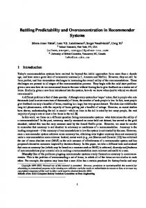
SOIL LANDSCAPE EVOLUTION I present here a case study of soil landscape evolution in the North Carolina coastal plain to show how NDS approaches can provide testable hypotheses relevant to both historical and process paradigms. The intimate relationships between pedological and geomorphological evolution are well described elsewhere (Birkeland 1984; Retallack 1990; McFadden and Kneupfer 1990; Gerrard 1992). The landscape-scale implications of chaotic pedogenesis and soil-landscape evolution have been discussed before (Arlinghaus et al. 1992; Culling 1988b; Ibanez et al. 1990; Phillips 1993b, c). The intent here is to show that an NDS-based analysis can generate testable hypotheses on specific soil-geomorphic phenomena. Textural Differentiation Model On the uplands of the North Carolina coastal plain (Figure 13.1), the most important factors defining the differences between soil types are the texture and thickness of A-, E-, and B-horizons. In the unconsolidated coastal plain sediments, under the prevailing humid subtropical climate, Ultisols are produced in all but the youngest sites, those subjected to dominantly regressive pedogenesis, or nearly pure sands. Textural differentiation is produced by chemical weathering and clay mineral synthesis in surficial (A- and E-horizons) and B-horizons, and by translocation via chemical dissolution-precipitation and lessivage. Differences in other soil properties, such as chemistry, structure, color, and consistency, arise as secondary impacts of textural differentiation, due to differences in drainage and degree of development, and in response to local variations in other soil-forming factors. A conceptual model of textural differentiation can be constructed to account for differences in the texture and thickness of A- and E- versus B-horizons. Critical components are the rate of clay synthesis in the A- and E-horizons, A, internal clay synthesis in the Bhorizon, B, the rate of eluvial loss from the surficial horizons, E, the rate of illuvial gain in the B-horizon, I, and the rate of moisture flux Ω. Units of clay synthesis and translocations

328

SCIENTIFIC NATURE OF GEOMORPHOLOGY

Figure 13.1 The North Carolina coastal plain. Triangles indicate sites of field soil geomorphology investigations used to develop or test the textural differential model

have dimensions of MT-1. Moisture flux in this case is the transmissitivity of the soil profile, with dimensions LT-1. A = cie-klA∆t

(5)

E = Ωc2A ∆t

(6)

I=E

(7)

B = c3e-k 3 B∆t

(8)

Ω = c4 -f (B ∆t + I∆t)

(9)

The c's are constants reflecting, respectively, the maximum A- and E-horizon clay mineral synthesis rate as controlled by climate and geochemistry; the removal rate from surface horizons associated with a given moisture flux; the maximum clay mineral synthesis rate in the B-horizon; and the moisture flux rate in the unaltered soil. The k's are coefficients describing, respectively, the decline in clay synthesis as clay accumulates in the surface and B-horizons. The equations reflect illuviation as a direct function of eluviation, clay accumulation in the surface horizons as synthesis minus eluvial loss, and accumulation in the subsurface as illuviation plus in situ synthesis. Eluvial loss from B-horizons occurs in the region, but is

DETERMINISTIC COMPLEXITY, EXPLANATION AND PREDICTABILITY

329

insignificant compared to the other processes. Weathering and clay synthesis rates slow as clay accumulates, due to depletion of weatherable minerals, though it might be argued for other situations that the increased water-holding capacity associated with accumulation of fines would increase weathering rates. Decline in clay synthesis is shown as a negative exponential function of clay accumulation, in accordance with earlier models of feedback effects in weathering. The moisture flux is shown as a generalized, unspecified negative function of subsoil clay accumulation. In eastern North Carolina, hydraulic conductivities of argillic horizons are typically half to less than a tenth of those in surface horizons. The specific form of these feedback functions is not important in this context; only that they are indeed negative functions. The relationships between the major components of the system are shown in Table 13.3. This interaction matrix gives only the positive, negative, or negligible (zero) influences of A, B, E, I, and Ω on each other, as reflected in the equations. The signs of the matrix elements are all that is necessary to determine whether there are any positive Lyapunov exponents. This method can therefore be used when exact (or generally applicable) relationships between system components cannot be specified, but the general nature of their interactions can be. Also, results are not dependent on any particular parameter values, or any particular form of the governing equations (Mendoza-Cabrales 1994; Phillips 1992a; Scheidegger 1993; Slingerland 1981). Variables a and β are not included, as they are linear combinations of other components. Links shown in the interaction matrix - a linearized version of the highly nonlinear equation system - include only the direct links - i.e. those that do not work through any other component. The coefficients of the characteristic polynomial of the matrix can be computed based on the feedback (F), where Fk =

Σ(-l)m+1L(m, k)

(10)

where k is the level or order and L(m, k) signifies m disjunct loops of total length k. Disjunct loops are sequences of aij (matrix elements) with no i or j in common. For example, feedback at level four (the fourth coefficient in the polynomial) would include all combinations of disjunct loops whose total length (number of components) is four. The Table 13.3 Interaction matrix showing the positive, negative, and negligible mutual influence in the soil textural differentiation model (A, E, I, B, Ω), respectively, represent rates of A- and Ehorizon clay synthesis, eluviation of clay from surficial horizons, illuviation in B-horizons, B-horizon clay synthesis, and moisture flux

A E I B Ω

A

E

-a11 0 0 0 0

a12 0 0 0 a52

I 0 a23 0 0 0

B 0 0 0 -a44 0

Ω 0 0 -a35 -a45 0

330

SCIENTIFIC NATURE OF GEOMORPHOLOGY

RHC criteria are that the system is stable (i.e. all eigenvalues have negative real parts and all λ < 0 if and only if Fk < 0 for all k, and (for n = 5):

F12 F4 + F1 F5 − F1 F2 F3 − F32 > 0 (11) In the textural differentiation system all Fk < 0, and the second stability criterion is also likely to be met. This implies that the system is stable to small perturbations and should not behave chaotically. However, this stability is contingent upon all relationships operating as shown in Table 13.3. If the role of clay accumulation in moisture storage to promote chemical weathering is stronger than the effects of mineral depletion, then equations (5) and (8) and the signs of a11 and a44 change, and the system becomes unstable. This could occur in early stages of weathering where the supply of weatherable minerals is not limiting, or where there is an influx of new weatherable minerals (for example, via deposition). There is also evidence that clay accumulation in the B-horizon does not necessarily limit eluviation or moisture flux, despite the clearly lower hydraulic conductivities in argillic horizons. The latter are typically on the order of 1.5 to 15 cm h-1 in coastal plain Ultisols. While this can limit movement during storm runoff, it is unlikely to inhibit water movement and eluviation over longer time scales. This would alter equation (9) and interaction matrix elements a34 and a45, and results in instability. Implications There are two major implications with respect to processes. The NDS analysis shows that two particular process mechanisms determine whether or not the system behaves chaotically. First, is the chemical weathering rate limited by the reaction rates or weatherable minerals? Second, do the hydraulic conductivity contrasts between the illuvial and overlying horizons limit eluviation (or the depth of illuviation)? These implications could clearly be tested in the field, and results could be linked to related hypotheses involving instability or spatial chaos-for example, where weathering is reaction-limited and depth of illuviation is not inhibited by B-horizon development, the spatial variability of soil profile morphologies and soil types in comparison to observable variation in controlling factors should be greater than where weathering is mineral-limited and eluviation-illuviation is inhibited. However, the process hypotheses do not need to be linked to NDS hypotheses to be useful, as they have intrinsic significance for landscape evolution. There is another major implication for soil landscape evolution. Where reaction rates are limiting and/or clay accumulation does not inhibit eluviation, the textural differentiation model is unstable and chaotic. If this is the case, then the spatial variability of the soil cover, in terms of the presence, texture, and thickness of A-, E-, and B-horizons in individual pedons, should increase over time. Soil cover on older soil landscapes should be more variable than that on younger ones, even where climate, biotic effects, parent material, and topography are very similar. This hypothesis has already been tested in an area of the lower North Carolina coastal plain where illuvial clay accumulation does not limit eluviation. The number of soil types, at the series level, was compared at two otherwise identical sites on adjacent geomorphic surfaces differing in age by about 150 000 years. The younger, late Pleistocene site had

DETERMINISTIC COMPLEXITY, EXPLANATION AND PREDICTABILITY

331

only one soil type while the older Pleistocene site had at least seven (Phillips 1993d). The hypothesis was thus not rejected. Given the fact that exponential divergence cannot last indefinitely, and the order and self-organization which must emerge at some scale in a chaotic system, there should be some broad-scale, regularities in the soil landscape, and a limit to the age of soil landscapes where increasing divergence is observed. The former is at least intuitively observed in the aggregate, coarse-scale predictability of the soil landscape model in the coastal plain. The latter can be tested if longer chronosequences can be developed. DISCUSSION AND CONCLUSIONS It is now clear that geomorphic systems are often complex, nonlinear, dynamical systems. That involves, in some cases, deterministic chaos and self-organization. However, applications of NDS theory to geomorphology have been hampered by three major problems: 1. Concepts and analytical techniques imported from mathematics and physics, where the simple, abstract systems bear little resemblance to real landscapes; 2. A lack of field tests; 3. Limited ability to provide explanations of geomorphic processes or evolution. The first problem is beginning to be solved by devising and adapting terminology and methodology appropriate to the geosciences (Ibanez et al. 1994; McBratney 1992; Phillips 1994; Zeng and Pielke 1993). The second can also apparently be overcome, as NDS theory has produced some field-testable hypotheses relevant to understanding surface processes and landscape evolution. The third will be-and I argue, is being-overcome to the extent NDS theory can explain geomorphic phenomena not otherwise explained, or produce testable hypotheses unlikely to be produced otherwise. In addition to examples from the literature, a case study shows NDS theory can be used to identify critical process mechanisms in soil formation and to provide a plausible explanation for soil landscapes where broad-scale regularities are overprinted with dramatic local-scale variability disproportionate to any variability in controlling factors. In general, while there are certainly inappropriate and unedifying applications of NDS theory in geomorphology, it has been shown in at least some cases to provide explanation, and to increase rather than decrease predictability. Whether that utility ultimately makes it just one of many useful perspectives for the geomorphologist or a perspective of preeminent importance remains to be seen. I believe that, whether or not geomorphologists explicitly embrace NDS theory and methods, the discipline is likely to continue to evolve: • Away from efforts to identify single, inevitable ultimate steady-state equilibria, and toward the recognition of inherently unstable and non-adjusting as well as steady-state 'climax' forms (see Renwich 1992). • Away from a linear cause-and-effect viewpoint whereby a given set of environmental controls produces a given landscape, and toward the recognition of multiple landscape responses and modes of adjustment.

332

SCIENTIFIC NATURE OF GEOMORPHOLOGY

• Away from perspectives which emphasize either the regularities or complexities in the landscape, and toward those which deal with both simultaneously, and which recognize order and stability as an emergent property of spatial and temporal scale. • Away from a view of unstable and nonsteady-state forms as anomalies or deviations from the norm, and toward a view where these are seen as norms in their own right. If these predictions are correct, then NDS theory is clearly an appropriate conceptual framework, but not necessarily the only appropriate one. Nonlinear systems approaches have at least one thing in common with any other conceptual framework, theory, or methodology: they do not, and cannot, answer or even address every question asked by geomorphologists. Given the prominence of NDS theory in science and its growing use in geomorphology, I argue that geomorphologists should have at least a passing acquaintance with NDS concepts. But those who do not 'do' NDS are not missing the boat, any more than those who do not do cosmogenic isotope dating, geoarcheology, or microprocess mechanics (for example). Nonlinear dynamical systems is unlikely to be the methodological or conceptual banner behind which all geomorphologists can rally, or the rubric under which all of geomorphology can be interpreted. It seems clear by now that there is probably no such banner or rubric (Rhoads and Thorn 1993). Whether NDS theory lives up to its promise depends in large measure on whether we promise, or expect, too much. REFERENCES Ahnert, F. 1994. Modelling the development of non-periglacial sorted nets, Catena, 23, 53-63. Arlinghaus, S.L., Nystuen, J.D. and Woldenberg, M.J. 1992. An application of graphical analysis to semidesert soils, Geographical Review, 82, 244-252. Bak, P., Tang, C. and Wiesenfeld, K. 1987. Self-organized criticality: an explanation of 1/f noise, Physical Review Letters, 59, 381-384. Birkeland, RW 1984. Soils and Geomorphology, Oxford University Press, New York, 372 pp. Brooks, D.R. and Wiley, E.O. 1988. Evolution as Entropy, 2nd edn., University of Chicago Press, 415 pp. Burrough, P.A. 1983. Multiscale sources of spatial variation in soils, Journal of Soil Science, 34, 577-620. Callander, R.A. 1969. Instability and river channels, Journal of Fluid Mechanics, 36, 465-480. Carlson, J.M., Chayes, J.T, Grannan, E.R. and Swindle, G.H. 1990. Self-organized critically and singular diffusion, Physical Review Letters, 65, 2547-2550. Carter, R.W.G and Orford, J. 1991. The sedimentary organization and behavior of drift-aligned barriers, Coastal Sediments '91, American Society Civil Engineers, New York, pp. 934-948. Chase, C.G. 1992. Fluvial landsculpting and the fractal dimension of topography, Geomorphology, 5, 39-57. Clifford, N.J. 1993. Formation of riffle-pool sequences: field evidence for an autogenic process, Sedimentary Geology, 85, 39-51. Culling, W.E.H. 1987. Equifinality: modern approaches to dynamical systems and their potential for geographical thought, Transactions, Institute of British Geographers, 12, 57-72. Culling, W.E.H. 1988a. A new view of the landscape, Transactions, Institute of British Geographers, 13, 345-360. Culling, W.E.H. 1988b. Dimension and entropy in the soil covered landscape, Earth Surface Processes and Landforms, 13, 619-648.

DETERMINISTIC COMPLEXITY, EXPLANATION AND PREDICTABILITY

333

DeBoer, D. 1992. Hierarchies and scale in process geomorphology: a review, Geomorphology, 4, 303-318. Elliott, J.K. 1989. An investigation of the change in surface roughness through time on the foreland of Austre Okstindbreen, North Norway, Computers and Geosciences, 15, 209-217. Ergenzinger, P. 1987. Chaos and order-the channel geometry of gravel bed braided rivers, Catena, supplement 10, 85-98. Gaffin, S.R. and Maasch, K.A. 1991. Anomalous cyclicity in climate and stratigraphy and modelling nonlinear oscillations, Journal of Geophysical Research, 96B, 6701-6711. Gerrard, A.J. 1992. Soil Geomorphology, Chapman and Hall, London, 269 pp. Haigh, M.J. 1988. Dynamic systems approaches in landslide hazard research, Zeitschrift für Geomorphologie, Supplement 67, 79-91. Hallet, B. 1990. Spatial self-organization in geomorphology: from periodic bedforms and patterned ground to scale-invariant topography, Earth-Science Reviews, 29, 57-75. Hooke, J.M. and Redmond, C.E. 1992. Causes and nature of river planform change, in Dynamics of Gravel-Bed Rivers, edited by P. Billi et al., Wiley, Chichester, pp. 559-571. Ibanez, J.J., Bellexta, R.J. and Alvarez, A.G. 1990. Soil landscapes and drainage basins in Mediterranean mountain areas, Catena, 17, 573-583. Ibanez, J.J., Perez-Gonzalez, A., Jimenez-Ballesta, R., Saldana, A. and Gallardo-Diaz, J. 1994. Evolution of fluvial dissection landscapes in Mediterranean environments: quantitative estimates and geomorphic, pedologic, and phytocenotic repercussions, Zeitschrift für Geomorphologie, 38, 105-119. Ijjasz-Vasquez, E.J., Bras, R.L. and Moglen, G.E. 1992. Sensitivity of a basin evolution model to the nature of runoff production and to initial conditions, Water Resources Research, 28, 2733-2741. Jayawardena, A.W. and Lai, F. 1994. Analysis and prediction of chaos in rainfall and streamflow time series, Journal of Hydrology, 153, 23-52. Kapitaniak, T. 1988. Chaos in Systems with Noise, World Scientific, Singapore, 189 pp. Kempel-Eggenberger, C. 1993. Risse in der geoökologischen Realität: Chaos und Ordnung in geoökologischen systemen, Erdkunde, 47, 1-11. Kramer, S. and Marder, M. 1992. Evolution of river networks, Physical Review Letters, 68, 205-208. Li, Q. and Nyland, E. 1994. Is the dynamics of the lithosphere chaotic? In Nonlinear Dynamics and Predictability of Geophysical Phenomena, edited by W.I. Newman et al., American Geophysical Union Geophysics Monograph, 83, pp. 37-41. Loewenherz, D.S. 1991. Stability and the initiation of channelized surface drainage: a reassessment of the short wavelength limit, Journal of Geophysical Research, 96B, 8453-8464. McBratney, A.B. 1992. On variation, uncertainty, and informatics in environmental soil management, Australian Journal of Soil Research, 30, 913-936. McFadden, L.D. and Knuepfer, P.L.K. (eds) 1990. Soils and Landscape Evolution, Elsevier, Amsterdam, 340 pp. McLean, S.R. 1990. The stability of ripples and dunes, Earth-Science Reviews, 29, 131-144. Malanson, G.P., Butler, D.R. and Georgakakos, K.P. 1992. Nonequilibrium geomorphic processes and deterministic chaos, Geomorphology, 5, 311-322. Malanson, G.P., Butler, D.R. and Walsh, S.J. 1990. Chaos in physical geography, Physical Geography, 11, 293-304. Masek, J.G. and Turcote, D.L. 1993. A diffusion-limited aggregation model for the evolution of drainage networks, Earth & Planetary Science Letters, 119, 379-386. Mayer, L. 1992. Some comments on equilibrium concepts and geomorphic systems, Geomorphology, 5, 277-295. Mendoza-Cabrales, C. 1994. Is bedform development chaotic? Hydraulic Engineering '94, American Society Civil Engineers, New York, pp. 78-81. Miller, S.T., Brinn, P.J., Fry, G.J. and Harris, D. 1994. Microtopography and agriculture in semi-arid Botswana. 1. Soil variability, Agricultural Water Management, 26, 107-132. Montgomery, K. 1993. Non-linear dynamics and river meandering, Area, 25, 97-108. Nahon, D.B. 1991. Self-organization in chemical lateritic weathering, Geoderma, 51, 5-13. Nelson, J.M. 1990. The initial instability and finite-amplitude stability of alternate bars in straight channels. Earth-Science Reviews, 29, 97-115.

334

SCIENTIFIC NATURE OF GEOMORPHOLOGY

Newman, W.I., Gabrielsou, A. and Turcotte, D. (eds) 1994. Nonlinear Dynamics and Predictability of Geophysical Phenomena, American Geophysical Union Geophysical Monograph 83. Nicoll, M.J., Wheatcroft, S.W., Tyler, S.W. and Berkowitz, B. 1994. Is Old Faithful a strange attractor? Journal of Geophysical Research, 99B, 4495-4503. Phillips, J.D. 1989. Erosion and planform irregularity of an estuarine shoreline, Zeitschrift für Geomorphologie, Supplement 73, 59-71. Phillips, J.D. 1990. The instability of hydraulic geometry, Water Resources Research, 26, 739-744. Phillips, J.D. 1992a. Qualitative chaos in geomorphic systems, with an example from wetland response to sea level rise, Journal of Geology, 100, 365-374. Phillips, J.D. 1992b. Deterministic chaos in surface runoff, in Overland Flow: Hydraulic and Erosion Mechanics, edited by A.J. Parson and A.D. Abrahams, University College London Press, London, pp.177-197. Phillips, J.D. 1992c. Nonlinear dynamical systems in geomorphology: revolution or evolution? In Geomorphic Systems, Proceedings of the Binghamton Geomorphology Symposium, edited by J.D. Phillips and W.H. Renwick, Elsevier, Amsterdam, pp. 219-229. Phillips, J.D. 1993a. Spatial-domain chaos in landscapes, Geographical Analysis, 25, 101-117. Phillips, J.D. 1993b. Stability implications of the state factor model of soils as a nonlinear dynamical system, Geoderma, 58, 1-15. Phillips, J.D. 1993c. Progressive and regressive pedogenesis and complex soil evolution, Quaternary Research, 40, 169-176. Phillips, J.D. 1993d. Chaotic evolution of some coastal plain soils, Physical Geography, 14, 566-580. Phillips, J.D. 1993d. Instability and chaos in hillslope evolution, American Journal of Science, 283, 25-48. Phillips, J.D. 1993f, Biophysical feedbacks and risk of desertification, Annals of the Association of American Geographers, 83, 630-640. Phillips, J.D. 1994. Determinstic uncertainty in landscapes, Earth Surface Processes and Landforms, 19, 389-401. Phillips, J.D. 1995a. Nonlinear dynamics and the evolution of relief, Geomorphology, 14, 57-64. Phillips, J.D. 1995b. Self-organization and landscape evolution, Progress in Physical Geography, 19, 309-321. Renwick, WH. 1992. Equilibrium, disequilibrium, and nonequilibrium landforms in the landscape, in Geomorphic Systems, Proceedings of the Binghamton Geomorphology Symposium, edited by J.D. Phillips and WH. Renwick, Elsevier, Amsterdam, pp. 265-276. Retallack, G. 1990. Soils of the Past, An Introduction to Paleopedology, Unwin-Hyman, London, 520 PP. Rhoads, B.L. and Thorn, C.E. 1993. Geomorphology as science: the role of theory, Geomorphology, 6, 287-307. Rigon, R., Rinaldo, A. and Rodriguez-Iturbe, I. 1994. On landscape self-organization, Journal of Geophysical Research, 99B, 11 971-11 993. Rinaldo, A., Rodriguez-Iturbe, I., Bras, R.L. and Ijjasz-Vasquez, E.J. 1993. Self-organized fractal river networks, Physical Review Letters, 70, 822-826. Saltzman, B. and Verbitsky, M. 1994. Late Pleistocene climatic trajectory in phase space of global ice, ocean state, and CO2: observations and theory. Paleoceanography, 90, 767-779. Scheidegger, A.E. 1983. The instability principle in geomorphic equilibrium, Zeitschrift für Geomorphologie, 27, 1-19. Selker, J.S., Steenhuis, T.S. and Parlange, Y.-S. 1992. Wetting front instability in homogeneous sandy soils under continuous infiltration, Soil Science Society of America Journal, 56, 1346-1350. Slingerland, R. 1981. Qualitative stability analysis of geologic systems with an example from river hydraulic geometry, Geology, 9, 491-493. Slingerland, R. 1989. Predictability and chaos in quantitative dynamic stratigraphy, in Quantitative Dynamic Stratigraphy, edited by T.A. Cross, Prentice-Hall, Englewood Cliffs, NJ, pp. 45-53. Slingerland, R. and Snow, R.S. 1988. Stability analysis of a rejuvenated fluvial system, Zeitschrift für Geomorphologie, Supplement 67, 93-102.

DETERMINISTIC COMPLEXITY, EXPLANATION AND PREDICTABILITY

335

Smith, T.R. and Bretherton, F.P. 1972. Stability and the conservation of mass in drainage basin evolution, Water Resources Research, 8, 1506-1529. Stark, C.P. 1991. An invasion percolation model of drainage network evolution, Nature, 352, 423-425. Stark, C.P. 1994. Cluster growth modelling of plateau erosion, Journal of Geophysical Research, 99B, 13 957-13 960. Takayasu, H. and Inaoka, H. 1992. New type of self-organized criticality in a model of erosion, Physical Review Letters, 68, 966-969. Thornes, J.B. 1988. Erosional equilibria under grazing, in Conceptual Issues in Archeology, edited by J.L. Bintliff et al., Edinburgh University Press, pp. 193-210. Turcotte, D.L. 1990. Implications of chaos, scale-invariance, and fractal statistics in geology, Global and Planetary Change, 89, 301-308. Turcotte, D.L. 1992. Fractals and Chaos in Geology and Geophysics, Cambridge University Press, New York, 221 pp. Werner, B.T. and Fink, T.M. 1994. Beach cusps as self-organized patterns, Science, 260, 968-971. Werner, B.T. and Hallet, B. 1993. Numerical simulation of self-organized stone stripes, Nature, 361, 142-145. Wilcox, B.P, Seyried, M.S. and Matison, T.H. 1991. Searching for chaotic dynamics of snowmelt runoff, Water Resources Research, 27, 1005-1010. Willgoose, G.R., Bras, R.L. and Rodriguez-Iturbe, I. 1991. A coupled channel network-growth and hillslope evolution model, Water Resources Research, 27, 1671-1696. Woldenberg, M.J. 1969. Spatial order in fluvial systems: Horton's laws derived from mixed hexagonal hierarchies of drainage basin areas, Geological Society of America Bulletin, 80, 97-112. Zdenkovic, M.L. and Scheidegger, A.E. 1989. Entropy of landscapes, Zeitschrift für Geomorphologie, 33, 361-371. Zeng, X. and Pielke, R.A. 1993. What does a low-dimensional weather attractor mean? Physics Letters A, 175, 299-304.