3. Regression & Exponential Smoothing - Department of Mathematics

3. Regression & Exponential Smoothing 3.1 Forecasting a Single Time Series Two main approaches are traditionally used to model a single time series z1 , z 2 , . . . , z n 1. Models the observation zt as a function of time as zt = f (t, β) + εt where f (t, β) is a function of time t and unknown coefficients β, and εt are uncorrelated errors.

1

∗ Examples: – The constant mean model: zt = β + εt – The linear trend model: zt = β0 + β1t + εt – Trigonometric models for seasonal time series zt = β0 + β1 sin

2π 2π t + β2 cos t + εt 12 12

2. A time Series modeling approach, the observation at time t is modeled as a linear combination of previous observations ∗ Examples: P

– The autoregressive model: zt = j≥1 πj zt−j + εt – The autoregressive and moving average model: p q P P zt = πj zt−j + θiεt−i + εt j=1

j=1

2

Discounted least squares/general exponential smoothing n X

wt[zt − f (t, β)]2

t=1

• Ordinary least squares: wt = 1. • wt = wn−t, discount factor w determines how fast information from previous observations is discounted. • Single, double and triple exponential smoothing procedures – The constant mean model – The Linear trend model – The quadratic model

3

3.2 Constant Mean Model zt = β + ε t • β: a constant mean level • εt: a sequence of uncorrelated errors with constant variance σ 2. If β, σ are known, the minimum mean square error forecast of a future observation at time n + l, zn+l = β + εn+l is given by zn(l) = β • E[zn+l − zn(l)] = 0, E[zn+1 − zn(l)]2 = E[ε2t ] = σ 2 • 100(1 − λ) percent prediction intervals for a future realization are given by [β − µλ/2σ; β + µλ/2σ] where µλ/2 is the 100(1 − λ/2) percentage point of standard normal distribution. 4

If β, σ are unknown, we use the least square estimate βˆ to replace β n

1X ˆ β = z¯ = zt n t=1 The l-step-ahead forecast of zn+l from time origin n by n X 1 zˆn(l) = z¯, σ ˆ2 = (zt − z¯)2 n − 1 t=1 2

2

2

• E[zn+l − zˆn(l)] = 0, Eˆ σ = σ , E[zn+1 − zˆn(l)] = σ

2

1+

1 n




• 100(1 − λ) percent prediction intervals for a future realization are given "    12  12 # by 1 1 ; β + tλ/2(n − 1)ˆ σ 1+ β − tλ/2(n − 1)ˆ σ 1+ n n where tλ/2(n − 1) is the 100(1 − λ/2) percentage point of t distribution with n − 1 degree of freedom. 5

• Updating Forecasts 1 1 (z1 + z2 + · · · + zn + zn+1) = [zn+1 + nˆ zn(1)] n+1 n+1 n 1 = zˆn(1) + zn+1 n+1 n+1 1 (zn+1 − zˆn(1)) = zˆn(1) + n+1

zˆn+1 =

• Checking the adequacy of the model Calculate the sample autocorrelation rk of the residuals zt − z¯ n P

rk =

(zt − z¯)(zt−k − z¯)

t=k+1 n P

,

k = 1, 2, . . .

(zt − z¯)2

t=1

If

√

n|rk | > 2: something might have gone wrong.

6

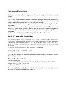
Example 3.1 Annual U.S. Lumber Production Consider the annual U.S. lumber production from 1947 through 1976. The data were obtained from U.S. Department of Commerce Survey of Current Business. The 30 observations are listed in Table Table 3.1: Annual Total U.S. Lumber Production (Millions of Broad Feet), 1947-1976 (Table reads from left to right) 35,404 37,462 32,901 33,178 34,449 38,044

36,762 36,742 33,385 34,171 36,124 38,658

32,901 36,356 32,926 35,697 34,548 32,087

38,902 37,858 32,926 35,697 34,548 32,087

37,515 38,629 32,019 35,710 36,693 37,153

7

Figure 3.1: Annual U.S. lumber production from 1947 to 1976(in millions of board feet) 4

4

x 10

3.9

Lumber production (MMbf)

3.8 3.7 3.6 3.5 3.4 3.3 3.2 3.1 3

1950

1955

1960

1965 Year

1970

1975

1980

8

• The plot of the data in Figure 3.1. • The sample mean and the sample standard deviation are given by 1 1 X z¯ = 35, 625, σ ˆ={ (zt − z¯)2} 2 = 2037 29

• The sample auto correlations of the observations are list below Lag k Sample autocorrelation

1 .20

2 -.05

3 .13

4 .14

5 .04

6 -.17

√ Comparing the sample autocorrelations with their standard error 1/ 30 = .18, we cannot find enough evidence to reject the assumption of uncorrelated error terms.

9

• The forecast from the constant mean model are the same for all forecast lead times and are given by zˆ1976(l) = z¯ = 35, 652 The standard error of these forecast is given by p σ ˆ 1 + 1/n = 2071 A 95 percent prediction interval is given by [35, 652 ± (2.045)(2071)] or

[31, 417, 39, 887]

• If new observation become available, the forecasts are easily updated. For example if Lumber production in 1977 was 37,520 million board feet. Then the revised forecasts are given by 1 zˆ1977(l) = zˆ1976(1) + [z1977 − zˆ1976(1)] n+1 1 = 35, 652 + [37, 520 − 35, 652] 31 10 = 35, 712

3.3 Locally Constant Mean Model and Simple Exponential Smoothing • Reason: In many instances, the assumption of a time constant mean is restrictive. It is more reasonable to allow for a mean that moves slowly over time • Method: Give more weight to the most recent observation and less to the observations in the distant past zˆn(l) = c

n−1 X

wtzn−t = c[zn + wzn−1 + · · · + wn−1z1]

t=0

w(|w| < 1): discount coefficient, c = (1 − w)/(1 − wn) is needed to normalized sum of weights to 1. • If n → ∞ and w < 1, then wn → 0, then X zˆn(l) = (1 − w) wj zn−j j≥0

11

• Smoothing constant: α = 1 − w. Smoothing statistics Sn = Sn[1] = (1 − w)[zn + wzn−1 + w2zn−2 + · · ·] = α[zn + (1 − α)zn−1 + (1 − α)2zn−2 + · · ·] • Updating Forecasts: (As easy as the constant mean model) Sn = (1 − w)zn + wSn−1 = Sn−1 + (1 − w)[zn − Sn−1] zˆn(1) = (1 − w)zn + wˆ zn−1(1) = zˆn−1(1) + (1 − w)[zn − zˆn−1(1)]

12

Actual Implementation of Simple Exp. Smoothing • Initial value for S0 Sn = (1 − w)[zn + wzn−1 + · · · + wn−1z1] + wnS0 . 1. S0 = z¯, (mean change slowly, α = 0); . 2. S0 = z1, (local mean changes quickly α = 1); 3. Backforecast ∗ , Sj∗ = (1 − w)zj + wSj+1

∗ = zn , Sn+1

S0 = z0 = S1∗ = (1 − w)z1 + wS2∗ • Choice of the Smoothing Constant: α = 1 − w et−1(1) = zt − zˆt−1(1) = zt − St−1, Then minimize

SSE(α) =

(one − step − ahead f orecast error). n X t=1

e2t−1(1).

13

• The smoothing constant that is obtained by simulation depends on the value of S0 • Ideally, since the choice of α depend on S0, one should choose α and S0 jointly • Examples – If α = 0, one should choose S0 = z¯. – If α = 1, one should choose S0 = z1 – If 0 < α < 1, one could choose S0 as the “backforecast” value: S0 = α[z1 + (1 − α)z2 + · · · + (1 − α)n−2zn−1] + (1 − α)n−1zn.

14

Example: Quarterly Iowa Nonfarm Income As an example, we consider the quarterly Iowa nonfarm income for 1948-1979. • The data exhibit exponential growth. • Instead of analyzing and forecasting the original series, we first model the quarterly growth rates of nonfarm income. zt =

It+1 − It It+1 100 ≈ 100 log It It

• The constant mean model would be clearly inappropriate. Compared with √ the standard error 1/ 127 = .089, most autocorrelations are significantly different from zero Table 3.2: Sample Autocorrelations rk of Growth Rates of Iowa Nofarm Income (n=127) Lag k Sample autocorrelation rk

1 .25

2 .32

3 .18

4 .35

5 .18

6 .22 15

Iowa nonfarm income, first quarter 1948 to fourth quarter 1979

6000

Iowa nofarm income (million $)

5000

4000

3000

2000

1000

0

1950

1955

1960

1965 Year

1970

1975

1980

16

Growth rates of Iowa nonfarm income, second quarter 1948 to fourth quarter 1979 5

4

Growth rate (%)

3

2

1

0

−1

−2

1950

1955

1960

1965 Year

1970

1975

1980

17

• Since the mean is slowly changing, simple exponential smoothing appears to be an appropriate method. • α = 0.11 and S0 = z¯ = 1.829. n P • SSE(.11) = e2t−1(1) = (−1.329)2 + (.967)2 + · · · + (.458)2 + (−.342)2 = 118.19

t=1

• As a diagnostic check, we calculate the sample autocorrelations of the one-step-ahead forecast errors n−1 P

rk =

[et(1) − e¯][et−k (1) − e¯]

t=k n−1 P

n−1

, [et(1) − e¯]2

1X e¯ = et(1). n t=0

t=0

• To assess the significance of the mean of the forecast errors, we compare it √ with standard error s/n1/2(1/ 127 = .089) , where n−1

1X 2 s = [et(1) − e¯]2 n t=0

18

19

20

21

22

3.4 Regression Models with Time as Independent Variable zn+j =

m X

βifi(j) + εn+j = f 0(j)β + εn+j

i=1

• f (j + 1) = Lf (j), L = (lij )m×m full rank. (Difference equations). • Equivalent model: zn+j =

m X

βi∗fi(n + j) + εn+j = f 0(n + j)β ∗ + εn+j ;

i=1

f (n + j) = Lnf (j) ⇒ β = Lnβ ∗. • Examples: Constant Mean Model, Linear Trend Model, Quadratic Trend Model, k th order Polynomial Trend Model, 12-point Sinusoidal Model

23

Pn ˆ • Estimation: βn minimizes j=1[zj − f 0(j − n)β]2 y0 = (z1, z2, . . . , zn), X0 X =

n−1 X

X0 = (f (−n + 1), . . . , f (0))

f (−j)f 0(−j)=F ˆ n,

X0 y =

j=0

n−1 X

f (−j)zn−j =h ˆ n

j=0

ˆ = F−1hn. β n n • Prediction ˆ , Var(en(l)) = σ 2[1 + f 0(l)F−1f (l)], zˆn(l) = f 0(l)β n n n−1 X 1 2 ˆ )2. σ ˆ = (zn−j − f 0(−j)β n n − m j=0

100(1 − λ)% CI :

0

−1

zˆn(l) ± tλ/2(n − m)ˆ σ [1 + f (l)F

1 2

f (l)] . 24

• Updating Estimates and Forecasts: −1 ˆ β = F n+1 n+1 hn+1 .

Fn+1 = Fn + f (−n)f 0(−n);

hn+1 =

n X

f (−j)zn+1−j = f (0)zn+1 +

j=0

n−1 X

f (−j − 1)zn−j

j=0

= f (0)zn+1 +

n−1 X

L−1f (−j)zn−j = f (0)zn+1 + L−1hn

j=0

ˆ zˆn+1(l) = f 0(l)β n+1 .

25

3.5 Discounted Least Square and General Exponential Smoothing In discounted least squares or general exponential smoothing, the parameter estimates are determined by minimizing n−1 X

wj [zn−j − f 0(−j)β]2

j=0

The constant w(|w| < 1) is a discount factor the discount past observation exponentially. Define W = diag(wn−1 wn−2 · · · w 1); n−1 X 0 Fn=X ˆ WX = wj f (−j)f 0(−j) j=0

hn=X ˆ 0Wy =

n−1 X j=0

wj f (−j)zn−j 26

• Estimation and Forecasts ˆ = F−1hn, β n n

ˆ . zˆn(l) = f 0(l)β n

• Updating Parameter Estimates and Forecasts −1 ˆ β n+1 = Fn+1 hn+1 ,

hn+1 =

n X

Fn+1 = Fn + f (−n)f 0(−n)wn;

wj f (−j)zn+1−j = f (0)zn+1 + wL−1hn

j=0

If n → ∞, then wnf (−n)f 0(−n) → 0, and Fn+1 = Fn + f (−n)f 0(−n)wn → F as n → ∞. Hence −1 0 −1 0 0 ˆ ˆ β = F f (0)z + [L − F f (0)f (0)L ]β n n+1 n+1

ˆ + F−1f (0)[zn+1 − zˆn(1)]. = L0β n ˆ zˆn+1(l) = f 0(l)β n+1 .

27

3.5 Locally Constant Linear Trend and Double Exp. Smoothing • Locally Constant Linear Trend Model zn+j = β0 + β1j + εn+j • Definition

F =

X

1 0 . 1 1 P j  " − P 2jwj = j w

f (j) = [1 j]0, L =

wj f (−j)f 0(−j) =







P j Pw j − jw

• Discount least squares that minimizing

n−1 P

1 1−w −w (1−w)2

−w (1−w)2 w(1+w) (1−w)2

#

wj [zn−j − f 0(−j)β]2, thus

j=1

" ˆ = F−1hn = β n

1−w

2 2

(1 − w)

2

(1 − w) (1−w)3 w

#

 P j Pw zjn−j − jw zn−j 28

Thus βˆ0,n = (1 − w )

X

βˆ1,n = (1 − w)2

X

2

j

2

w zn−j − (1 − w)

X

jwj zn−j

3X (1 − w) wj zn−j − jwj zn−j w

In terms of smoothing Sn[1]

= (1 − w)zn +

[1] wSn−1

wj zn−j , X 2 = (1 − w) (j + 1)wj zn−j ,

= (1 − w)

[2]

Sn[2] = (1 − w)Sn[1] + wSn−1

X

[k]

Sn[k] = (1 − w)Sn[k−1] + wSn−1. (Sn[0] = (no smoothing) = zn) Then βˆ0,n = 2Sn[1] − Sn[2], 1 − w [1] (Sn − Sn[2]). βˆ1,n = w 1 − w [1] 1 − w [2] ˆ ˆ zˆn(l) = β0,n + β1,n · l = (2 + l)Sn − (1 + l)Sn . w w

29

• Updating: βˆ0,n+1 = βˆ0,n + βˆ1,n + (1 − w2)[zn+1 − zˆn(1)], βˆ1,n+1 = βˆ1,n + (1 − w)2[zn+1 − zˆn(1)]; Or in another combination form: βˆ0,n+1 = (1 − w2)zn+1 + w2(βˆ0,n + βˆ1,n), 1−w ˆ 2w ˆ ˆ ˆ β1,n+1 = (β0,n+1 − β0,n) + β1,n. 1+w 1+w 1 zn+1 − zˆn(1) = (βˆ0,n+1 − βˆ0,n − βˆ1,n). 2 1−w

30

• Implementation [2]

[1]

– Initial Values for S0 and S0 [1]

S0

[2]

S1

w ˆ β1,0, 1−w 2w ˆ ˆ β1,0; = β0,0 − 1−w = βˆ0,0 −

where the (βˆ0,0, βˆ1,0) are usually obtained by considering a subset of the data fitted by the standard model zt = β0 + β1t + εt. – Choice of the Smoothing Constant α = 1 − w The smoothing constant α is chosen to minimize the SSE: X SSE(α) = (zt − zˆt−1)2     2 X α α [1] [2] = zt − 2 + St−1 + 1 + St−1 . 1−α 1−α

31

Example: Weekly Thermostat Sales As an example for double exponential smoothing, we analyze a sequence of 52 weekly sales observations. The data are listed in Table and plotted in Figure. The data indicates an upward trend in the thermostat sales. This trend, however, does not appear to be constant but seems to change over time. A constant linear trend model would therefore not be appropriate. Case Study II: University of Iowa Student Enrollments As another example, we consider the annual student enrollment (fall and spring semester combined) at the University of Iowa. Observations for last 29 years (1951/1952 through 1979/1980) are summarized in Table. A plot of the observations is given in Figure.

32

33

400

Thermostat Sales

350

300

250

200

150

100 0

5

10

15

20

25 30 Week

35

40

45

50

55

Weekly thermostat sales

34

35

36

37

38

3.6 Regression and Exponential Smoothing Methods to Forecast Seasonal Time Series • Seasonal Series: Series that contain seasonal components are quite common, especially in economics, business, and the nature sciences. • Much of seasonality can be explained on the basis of physical reasons. The earth’s rotation around the sun, for example, introduces a yearly seasonal pattern into may of the meteorological variables. • The seasonal pattern in certain variables, such as the one in meteorological variables, is usually quite stable and deterministic and repeats itself year after year. The seasonal pattern in business and economic series, however, is frequently stochastic and changes with time. • Apart from a seasonal component, we observe in many series an additional trend component. 39

40

41

42

The traditional approach to modeling seasonal data is to decompose the series into three components: a trend Tt, a seasonal component St and an irregular (or error) component εt • The additive decomposition approach zt = T t + S t + ε t • The multiplicative decomposition approach zt = T t × S t × ε t or log zt = Tt∗ + St∗ + ε∗t • The other multiplicative model zt = T t × S t + ε t 43

3.6.1 Globally Constant Seasonal Models Consider the additive decomposition model zt = Tt + St + εt • Traditionally the trend component Tt is modeled by low-order polynomials k of time t: X ti Tt = β0 + βi i! i=1 • The seasonal component St can be described by seasonal indicators St =

s X

δiINDti

i=1

where INDti = 1 if t corresponds to the seasonal period i, and 0 otherwise, or by trigonometric functions m X

2πi St = Ai sin( t + φi). s i=1 where Ai and φi are amplitude and the phase shift of the sine function with frequency fi = 2πi/s. 44

Modeling the Additive Seasonality with Seasonal Indicators k X

s

ti X zt = β0 + βi + δiINDti + εt. i! i=1 i=1 Since it uses s + 1 parameters ( β0 and s seasonal indicators) to model s seasonal intercepts, restrictions have to be imposed before the parameters can be estimated. Several equivalent parameterizations are possible • Omit the intercept: β0 = 0. • Restrict

Ps

i=1 δi

= 0.

• Set one of the δ’s equal to zero; for example δs = 0. Mathematically these modified models are equivalent, but for convenience we usually choose (3).

45

Now we have the standard regression model: k X

s−1

ti X zt = β0 + βi + δiINDti + εt. i! i=1 i=1 β 0 = (β0, β1, . . . , βk , δ1, . . . , δs−1); Hence βˆ = (XX0)−1X0y,

y0 = (z1, z2, . . . , zn);

X is an n × (k + s)matrix with tth row given by   2 k t t f 0(t) = 1, t, , · · · , , INDt1, · · · , INDt,s−1 2 k! The minimum mean square error forecast of zn+l can be calculated from ˆ zˆn(l) = f 0(n + l)β 100(1 − α)% prediction interval 0

0 −1

zˆn(l) ± tλ/2(n − k − s)ˆ σ [1 + f (n + l)(XX ) where

n X 1 ˆ 2. σ ˆ2 = (zt − f 0(t)β) n − k − s t=1

1 2

f (n + l)] , 46

Change of Time Origin in the Seasonal Indicator Model As we mentioned in previous sections, it might be easier to update the estimates/ prediction if we use the last observational time n as the time origin. In this case k s−1 X ji X zn+j = β0 + βi + δiINDji + εn+j . i! i=1 i=1   2 k j j 0 f (j) = 1, j, , · · · , , INDj1, · · · , INDj,s−1 2 k! ˆ = F−1hn β n

Fn =

n−1 X

f (−j)f 0(−j),

n

, hn =

j=0

n−1 X

f (−j)zn−j .

j=0

Hence the prediction: ˆ zˆn(l) = f 0(l)β 100(1 − α)% prediction interval 1

2 zˆn(l) ± tλ/2(n − k − s)ˆ σ [1 + f 0(l)F−1 n f (l)] ,

47

It can be shown that the forecast or fitting functions follow the difference equation f (j) = Lf (j − 1), where L is a (k + s) × (k + s) transition matrix  L=

L11 0 L21 L22



As an illustration, let us consider a model with quadratic trend and seasonal period s = 4 3

zn+j

j2 X = β0 + β1 + β2 + δiINDji + εn+j 2 i=1

Then the transition matrix L and the initial vector f (0) are given by 

L11



1 0 0 = 1 1 0  1/2 1 1



L21



1 0 0 = 0 0 0  0 0 0



L22



−1 −1 −1 0 0  = 1 0 1 0

Successive application of the difference equation f (j) = Lf (j − 1) leads to f (j) = (1, j, j 2/2, INDj1, INDj2, INDj3)0. 48

Modeling the Seasonality with Trigonometric Functions k X

  m ti X 2πi zt = Tt + St + εt = β0 + βi + Ai sin t + φi + εt, i! s i=1 i=1 where the number of harmonics m should not goes beyond s/2, i.e. half the seasonality. Monthly, quarterly data; s/2 harmonics are usually not necessary This is illustrated in Figure, where we plot

E(zt) =

2 X i=1

 Ai sin

2πi t + φi 12



for A1 = 1, φ1 = 0, A2 = −0.70, φ2 = .6944π.

49

50

Change of Time Origin in the Seasonal Trigonometric Model Examples: • 12-point sinusoidal model (k = 0, s = 12, m = 1) zn+j = β0 + β11 sin

2πj 2πj + β21 cos + εn+j 12 12

In this case: 



1 √0 0 3/2 √1/2  , L= 0 0 −1/2 3/2





1 f (0) =  0  1

• Linear trend model with two superimposed harmonics (k = 1, s = 12, m = 2): zn+j

2πj 2πj 4πj 4πj = β0 +β1j +β11 sin +β21 cos +β12 sin +β22 cos +εn+j 12 12 12 12 51

3.6.2 Locally Constant Seasonal Models zn+j = f 0(j)β + εn+j • Target: Minimizing

S(β, n) =

n−1 X

wj [zn−j − f 0(−j)β]2

j=0

• updating: 0ˆ

ˆ β n+1 = L β n + F

−1

f (0)[zn+1 − zˆn(1)],

(F =

X

wj f 0(−j)f (−j))

j≥0

• A collection of infinite sums needed to cacluate F for seasonal models is given in the following Table. 52

53

• It is usually suggested that the least squares estimate of β in the regression ˆ . model zt = f 0(t)β + εt be taken as initial vector β 0 • To update the estimates, a smoothing constant must be determined. – As Brown (1962) suggest that the value of w should lie between (.70)1/g and (.95)1/g – If sufficient historical data are available, one can estimate w = 1 − α by simulation and choose the smoothing constant that minimizes the sum of the squared one-step-ahead forecast errors SSE(α) =

n X

[zt − zˆt−1(1)]2

t=1

• After estimating the smoothing constant α, one should always check the adequacy of the model. The sample autocorrelation function of the onestep-ahead forecast errors should be calculated . Significant autocorrelations indicate that the particular forecast model is not appropriate. 54

Locally Constant Seasonal Models Using Seasonal Indicators

zn+j = β0 + β1j +

3 X

δiINDji + εn+j = f 0(j)β

i=1

where f (j) = [1 j INDj1 INDj2 INDj3]0, f (0) = [1 0 0 0 0]0. Then    L=  

1 1 1 0 0



0 0 0 0 1 0 0 0   0 −1 −1 −1   0 1 0 0  0 0 1 0

Hence the updating weights in 0ˆ −1 ˆ β = L β + F f (0)[zn+1 − zˆn(1)] n+1 n

can be calculated from f (0) and the symmetric matrix 55



1 1−w

    F=   

w3 1−w4 −w3 (3+w4 ) (1−w4 )2 w3 1−w4

−w (1−w)2 w(1+w) (1−w)3

symmetric

w2 1−w4 −w2 (2+2w4 ) (1−w4 )2

w 1−w4 −w(1+3w4 ) (1−w4 )2

0

0

w2 1−w4

0 w 1−w4

        

Implications of α → 1 In this situation F →singular as w → 0. But we have that −1

lim F

w→0

f

∗

= f =



s−1 1 1 2 1, , − , − , · · · , − s s s s

0 ;

0ˆ ∗ ˆ β ˆn(1)]; n+1 = L β n + f [zn+1 − z

zˆn(1) = zn + zn+1−s − zn−s = zn+1−s + (zn − zn−s) zˆn(l) = zˆn(l − 1) + zˆn(l − s) − zˆn(l − s − 1) 56

Example: Car Sales Consider the monthly car sales in Quebec from January 1960 through December 1967 (n = 96 observations). The remaining 12 observations (1968) are used as a holdcut period to evaluate the forecast performance. An initial inspection of the series in Figure shows the data may be described by an additive model with a linear trend (k = 1) and a yearly seasonal pattern; the trend and the seasonal components appear fairly constant.

zt = β0 + β1t +

11 X

δiINDti + εt.

i=1

57

30

25

Car sales (1000s)

20

15

10

5

0 1960

1961

1962

1963

1964 1965 1966 1967 1968 1969 Year Figure: Monthly car sales in Quebec, Canada; January 1960 to December 1968

58

59

60

61

62

63

64

Example: New Plant and Equipment Expenditures Consider quarterly new plant and equipment expenditures for the first quarter of 1964 through the fourth quarter of 1974 (n = 44). The time series plot in Figure indicate s that the size of the seasonal swings increases with the level of the series; hence a logarithmic transformation must considered. The next Figure shows that this transformation has stabilized the variance.

zt = ln yt = β0 + β1 +

3 X

δiINDti + εt

i=1

65

New plant and equipment expenditures (billion $)

40 35 30 25 20 15 10 5 0 1964

1966

1968

1970 1972 1974 1976 Year Figure: Quarterly new plant and equipment expenditure in U.S. industries (in billions of dollars), first quarter 1 to fourth quarter 1976

66

Logarithm of new plant and equipment expenditures

3.4 3.2 3 2.8 2.6 2.4 2.2 1964

1966

1968

1970 1972 1974 1976 Year Logarithm of quarterly new plant and equipment expenditures, frist quarter 1964 to fourth quarter 1976

67

68

69

70

71

72

73

74