3D Face Tracking and Learning with Generative Models A dissertation ...

UNIVERSITY OF CALIFORNIA, SAN DIEGO Facing Uncertainty: 3D Face Tracking and Learning with Generative Models A dissertation submitted in partial satisfaction of the requirements for the degree Doctor of Philosophy in Cognitive Science by Tim Kalman Marks

Committee in charge: James Hollan, Chair Javier Movellan, Co-Chair Garrison Cottrell Virginia de Sa Geoffrey Hinton Terrence Sejnowski Martin Sereno

2006

Copyright Tim Kalman Marks, 2006 All rights reserved.

The dissertation of Tim Kalman Marks is approved, and it is acceptable in quality and form for publication on microfilm:

Co-Chair Chair

University of California, San Diego 2006

iii

To my wife, the light and love of my life, who throughout the difficult process of writing this dissertation has brought me not only dinner at the lab, but also much joy and comfort.

iv

TABLE OF CONTENTS Signature Page . . . . . . . . . . . . . . . . . . . . . . . . . . . . . . . . . . . .

iii

Dedication . . . . . . . . . . . . . . . . . . . . . . . . . . . . . . . . . . . . . . .

iv

Table of Contents . . . . . . . . . . . . . . . . . . . . . . . . . . . . . . . . . . .

v

List of Figures . . . . . . . . . . . . . . . . . . . . . . . . . . . . . . . . . . . . viii List of Tables . . . . . . . . . . . . . . . . . . . . . . . . . . . . . . . . . . . . .

ix

Acknowledgements . . . . . . . . . . . . . . . . . . . . . . . . . . . . . . . . . .

x

Vita and Publications . . . . . . . . . . . . . . . . . . . . . . . . . . . . . . . .

xi

Abstract of the Dissertation . . . . . . . . . . . . . . . . . . . . . . . . . . . . . xii Notation I

. . . . . . . . . . . . . . . . . . . . . . . . . . . . . . . . . . . . . . .

Introduction . . . . . . . . . . . . . . . . . . . . . . . . . . . . . . . . . . . . I.1 Overview of the thesis research . . . . . . . . . . . . . . . . . . . . . . I.1.1 G-flow: A Generative Probabilistic Model for Video Sequences I.1.2 Diffusion Networks for automatic discovery of factorial codes . I.2 List of Findings . . . . . . . . . . . . . . . . . . . . . . . . . . . . . . .

. . . . .

. 2 . 5 . 5 . 9 . 11

II Joint 3D Tracking of Rigid Motion, Deformations, and Texture using a Conditionally Gaussian Generative Model . . . . . . . . . . . . . . . . . . . . . . . . II.1 Introduction . . . . . . . . . . . . . . . . . . . . . . . . . . . . . . . . . . . II.1.1 Existing systems for nonrigid 3D face tracking . . . . . . . . . . . II.1.2 Our approach . . . . . . . . . . . . . . . . . . . . . . . . . . . . . . II.1.3 Collecting video with locations of unmarked smooth features . . . II.2 Background: Optic flow . . . . . . . . . . . . . . . . . . . . . . . . . . . . II.3 The Generative Model for G-Flow . . . . . . . . . . . . . . . . . . . . . . II.3.1 Modeling 3D deformable objects . . . . . . . . . . . . . . . . . . . II.3.2 Modeling an image sequence . . . . . . . . . . . . . . . . . . . . . II.4 Inference in G-Flow: Preliminaries . . . . . . . . . . . . . . . . . . . . . . II.4.1 Conditionally Gaussian processes . . . . . . . . . . . . . . . . . . II.4.2 Importance sampling . . . . . . . . . . . . . . . . . . . . . . . . . . II.4.3 Rao-Blackwellized particle filtering . . . . . . . . . . . . . . . . . . II.5 Inference in G-flow: A bank of expert filters . . . . . . . . . . . . . . . . . II.5.1 Expert Texture Opinions . . . . . . . . . . . . . . . . . . . . . . . II.5.1.1 Kalman equations for dynamic update of texel maps . . II.5.1.2 Interpreting the Kalman equations . . . . . . . . . . . . .

v

1

14 15 17 20 21 23 25 26 27 31 31 32 34 35 36 37 38

II.6

II.7 II.8

II.9

II.A

II.B

II.C

II.5.2 Expert Pose opinions . . . . . . . . . . . . . . . . . . . . . . . . . . II.5.2.1 Gaussian approximation of each expert’s pose opinion . . II.5.2.2 Importance sampling correction of the Gaussian approximation . . . . . . . . . . . . . . . . . . . . . . . . . . . . II.5.3 Expert credibility . . . . . . . . . . . . . . . . . . . . . . . . . . . . II.5.4 Combining Opinion and Credibility to estimate the new filtering distribution . . . . . . . . . . . . . . . . . . . . . . . . . . . . . . . II.5.5 Summary of the G-flow inference algorithm . . . . . . . . . . . . . Relation to optic flow and template matching . . . . . . . . . . . . . . . . II.6.1 Steady-state texel variances . . . . . . . . . . . . . . . . . . . . . . II.6.2 Optic flow as a special case . . . . . . . . . . . . . . . . . . . . . . II.6.3 Template Matching as a Special Case . . . . . . . . . . . . . . . . II.6.4 General Case . . . . . . . . . . . . . . . . . . . . . . . . . . . . . . Invisible face painting: Marking and measuring smooth surface features without visible evidence . . . . . . . . . . . . . . Results . . . . . . . . . . . . . . . . . . . . . . . . . . . . . . . . . . . . . . II.8.1 Comparison with constrained optic flow: Varying the number of experts . . . . . . . . . . . . . . . . . . . . II.8.2 Multiple experts improve initialization . . . . . . . . . . . . . . . . II.8.3 Exploring the continuum from template to flow: Varying the Kalman gain . . . . . . . . . . . . . . . . . . . . . . . II.8.4 Varying the Kalman gain for different texels . . . . . . . . . . . . . II.8.5 Implementation details . . . . . . . . . . . . . . . . . . . . . . . . . II.8.6 Computational complexity . . . . . . . . . . . . . . . . . . . . . . . Discussion . . . . . . . . . . . . . . . . . . . . . . . . . . . . . . . . . . . . II.9.1 Relation to previous work . . . . . . . . . . . . . . . . . . . . . . . II.9.1.1 Relation to other algorithms for tracking 3D deformable objects . . . . . . . . . . . . . . . . . . . . . . . . . . . . II.9.1.2 Relation to Jacobian images of texture maps . . . . . . . II.9.1.3 Relation to other Rao-Blackwellized particle filters . . . . II.9.2 Additional contributions . . . . . . . . . . . . . . . . . . . . . . . . II.9.3 Future work . . . . . . . . . . . . . . . . . . . . . . . . . . . . . . . II.9.4 Conclusion . . . . . . . . . . . . . . . . . . . . . . . . . . . . . . . Appendix: Using infrared to label smooth features invisibly . . . . . . . . II.A.1 Details of the data collection method . . . . . . . . . . . . . . . . . II.A.2 The IR Marks data set for 3D face tracking . . . . . . . . . . . . . Appendix: Exponential rotations and their derivatives . . . . . . . . . . . II.B.1 Derivatives of rotations . . . . . . . . . . . . . . . . . . . . . . . . II.B.2 Derivatives of a vertex location in the image . . . . . . . . . . . . . Appendix: Gauss-Newton and Newton-Raphson Optimization . . . . . . . II.C.1 Newton-Raphson Method . . . . . . . . . . . . . . . . . . . . . . . II.C.2 Gauss-Newton Method . . . . . . . . . . . . . . . . . . . . . . . . . II.C.2.1 Gauss-Newton approximates Newton-Raphson . . . . . . vi

39 39 42 43 45 45 49 49 50 52 53 55 56 56 56 59 59 61 64 64 64 64 70 70 71 72 74 76 77 81 84 85 86 87 87 88 88

II.D

II.E

II.F II.G II.H

II.C.2.2 Gauss-Newton approximates ρ using squares of linear terms 90 Appendix: Constrained optic flow for deformable 3D objects . . . . . . . 91 II.D.1 Derivatives with respect to translation . . . . . . . . . . . . . . . . 92 II.D.2 Derivatives with respect to morph coefficients . . . . . . . . . . . . 93 II.D.3 Derivatives with respect to rotation . . . . . . . . . . . . . . . . . 93 II.D.4 The Gauss-Newton update rules . . . . . . . . . . . . . . . . . . . 94 Appendix: The Kalman filtering equations . . . . . . . . . . . . . . . . . . 95 II.E.1 Kalman equations for dynamic update of background texel maps . 96 II.E.2 Kalman equations in matrix form . . . . . . . . . . . . . . . . . . . 96 Appendix: The predictive distribution for Yt . . . . . . . . . . . . . . . . . 97 Appendix: Estimating the peak of the pose opinion . . . . . . . . . . . . . 100 Appendix: Gaussian estimate of the pose opinion distribution . . . . . . . 101 II.H.1 Hessian matrix of ρobj with respect to δ . . . . . . . . . . . . . . . 102 II.H.2 Sampling from the proposal distribution . . . . . . . . . . . . . . . 103

III Learning Factorial Codes with Diffusion Neural Networks . . . . . . . . III.1 Introduction . . . . . . . . . . . . . . . . . . . . . . . . . . . . . . . III.2 Diffusion networks . . . . . . . . . . . . . . . . . . . . . . . . . . . III.2.1 Linear diffusions . . . . . . . . . . . . . . . . . . . . . . . . III.3 Factor analysis . . . . . . . . . . . . . . . . . . . . . . . . . . . . . III.4 Factorial diffusion networks . . . . . . . . . . . . . . . . . . . . . . III.4.1 Linear factorial diffusion networks . . . . . . . . . . . . . . III.5 Factor analysis and linear diffusions . . . . . . . . . . . . . . . . . III.6 A diffusion network model for PCA . . . . . . . . . . . . . . . . . . III.7 Training Factorial Diffusions . . . . . . . . . . . . . . . . . . . . . . III.7.1 Contrastive Divergence . . . . . . . . . . . . . . . . . . . . III.7.2 Application to linear FDNs . . . . . . . . . . . . . . . . . . III.7.3 Constraining the diagonals to be positive . . . . . . . . . . III.7.4 Positive definite update rules . . . . . . . . . . . . . . . . . III.7.4.1 The parameter rh as a function of woh and ro . . . III.7.4.2 The update rules for ro and woh . . . . . . . . . . III.7.4.3 Diagonalizing rh . . . . . . . . . . . . . . . . . . . III.8 Simulations . . . . . . . . . . . . . . . . . . . . . . . . . . . . . . . III.8.1 Learning the structure of 3D face space . . . . . . . . . . . III.8.2 Inferring missing 3D structure and texture data . . . . . . . III.8.2.1 Inferring the texture of occluded points . . . . . . III.8.2.2 Determining face structure from key points . . . . III.8.3 Advantages over other inference methods . . . . . . . . . . III.9 Learning a 3D morphable model from 2D data using linear FDNs III.10 Future directions . . . . . . . . . . . . . . . . . . . . . . . . . . . . III.11 Summary and Conclusions . . . . . . . . . . . . . . . . . . . . . .

vii

. . . . . . . . . . . . . . . . . . . . . . . . . .

. . . . . . . . . . . . . . . . . . . . . . . . . .

. . . . . . . . . . . . . . . . . . . . . . . . . .

. . . . . . . . . . . . . . . . . . . . . . . . . .

105 106 111 111 112 113 113 115 118 120 120 122 123 124 125 125 127 128 128 131 132 133 136 138 139 141

LIST OF FIGURES I.1 I.2

Reverend Thomas Bayes . . . . . . . . . . . . . . . . . . . . . . . . . . . . Diffusion networks and their relationship to other approaches . . . . . . .

II.1 II.2 II.3 II.4 II.5 II.6 II.7 II.8

A single frame of video from the IR Marks dataset Image rendering in G-flow . . . . . . . . . . . . . . Graphical model for G-flow video generation . . . . The continuum from flow to template . . . . . . . The advantage of multiple experts . . . . . . . . . G-flow tracking an outdoor video . . . . . . . . . . Varying the Kalman gain . . . . . . . . . . . . . . Varying Kalman gain within the same texture map

. . . . . . . .

. . . . . . . .

. . . . . . . .

. . . . . . . .

. . . . . . . .

. . . . . . . .

. . . . . . . .

. . . . . . . .

. . . . . . . .

. . . . . . . .

22 28 29 54 57 58 60 62

III.1 III.2 III.3 III.4 III.5 III.6 III.7 III.8

A Morton-separable architecture . . . . . . . . . . . . . . The USF Human ID 3D face database . . . . . . . . . . . Linear FDN hidden unit receptive fields for texture . . . . LInear FDN hidden unit receptive fields for structure . . . Reconstruction of two occluded textures . . . . . . . . . . Inferring the facestructure from key points . . . . . . . . . Failure of the SVDimpute algorithm . . . . . . . . . . . . Two routes to non-Gaussian extensions of the linear FDN.

. . . . . . . .

. . . . . . . .

. . . . . . . .

. . . . . . . .

. . . . . . . .

. . . . . . . .

. . . . . . . .

. . . . . . . .

. . . . . . . .

108 129 130 131 134 135 138 140

viii

. . . . . . . .

. . . . . . . .

. . . . . . . .

5 9

LIST OF TABLES II.1 Overview of Inference in G-flow . . . . . . . . . . . . . . . . . . . . . . . . 36 II.2 Approaches to 3D tracking of deformable objects . . . . . . . . . . . . . . 65

ix

ACKNOWLEDGEMENTS I have been privileged to work with my research advisor, Javier Movellan, for the past 6 years. From Javier I have learned a great deal about probability theory and machine learning, as well as how to have a passion for mathematical and scientific beauty. My Department advisor, Jim Hollan, has given me a great deal of helpful advice and support over the past seven and a quarter years. Jim’s advice about life, education, and career has been invaluable. I would also like to thank the rest of my committee for all of the time and effort they have put in, and for their helpful suggestions to improve this dissertation. Science is a team sport, and doing research with others is often more rewarding and more enlightening than working only on one’s own. I have had particularly fruitful and enjoyable research collaboration with John Hershey, and have had particularly fruitful and enjoyable study sessions with David Groppe. I would also like to thank everyone at the Machine Perception Lab (especially Ian Fasel, Marni Bartlett, Gwen Littlewort Ford, and Cooper Roddey), and everyone at the Distributed Cognition and Human-Computer Interaction Lab (especially Ed Hutchins) for fascinating discussions, helpful suggestions, support, and kind words. Other friends I would like to thank include Sam Horodezky, Jonathan Nelson, Laura Kemmer, Wendy Ark, Irene Merzlyak, Chris Cordova, Bob Williams, Ayse Saygin, Flavia Filimon, and many other fellow students that have lent their support over the years. I am grateful to my parents for their unconditional love, constant support, and encouragement. Finally, my thanks, as well as all of my love, go to my wife. Her friendship, love, and support have made it all worthwhile, not to mention a lot easier. Tim K. Marks was supported by: Darpa contract N66001-94-6039, the National Defense Science and Engineering Graduate (NDSEG) Fellowship, NSF grant IIS-0223052, and NSF grant DGE-0333451 to GWC.

x

VITA 1991

A.B., cum laude, Harvard University

1991–1994

Teacher, Glenbrook South High School

1995–1998

Editor, Houghton Mifflin/McDougal Littell

1999–2002

National Defense Science and Engineering Graduate Fellowship

2001

M.S., University of California San Diego

2002–2003

Head Teaching Assistant, Cognitive Science, UCSD

2004–2005

National Science Foundation IGERT Fellowship

2006

Ph.D., University of California San Diego PUBLICATIONS

Marks, T.K., Hershey, J., Roddey, J.C., and Movellan, J.R. Joint Tracking of Pose, Expression, and Texture using Conditionally Gaussian Filters. Neural Information Processing Systems 17 (NIPS 2004). Marks, T.K., Hershey, J., Roddey, J.C., and Movellan, J.R. 3D Tracking of Morphable Objects Using Conditionally Gaussian Nonlinear Filters. IEEE Computer Vision and Pattern Recognition (CVPR 2004), Generative Model-Based Vision (GMBV) Workshop. Marks, T.K., Roddey, J.C., Hershey, J., and Movellan, J.R. Determining 3D Face Structure from Video Images using G-Flow. Demo, Neural Information Processing Systems 16 (NIPS 2003). Movellan, J.R., Marks, T.K., Hershey, J., and Roddey, J.C. G-flow: A Generative Model for Tracking Morphable Objects. DARPA Human ID Workshop, September 29–30, 2003. Marks, T.K., Roddey, J.C., Hershey, J., and Movellan, J.R. G-Flow: a Generative Framework for Nonrigid 3D tracking. Proceedings of 10th Joint Symposium on Neural Computation, 2003. Marks, T.K. and Movellan, J.R. Diffusion Networks, Product of Experts, and Factor Analysis. Proceedings of 3rd International Conference on Independent Component Analysis and Blind Signal Separation, 2001. Fasel, I.R. and Marks, T.K. Smile and Wave: A Comparison of Gabor Representations for Facial Expression Recognition. 10th Joint Symposium on Neural Computation, 2001. Marks, T.K., Mills, D.L., Westerfield, M., Makeig, S., Jung, T.P., Bellugi, U., and Sejnowski, T.J. Face Processing in Williams Syndrome: Using ICA to Discriminate Functionally Distinct Independent Components of ERPs in Face Recognition. Proceedings of 7th Joint Symposium on Neural Computation, pp. 55–63, 2000.

xi

ABSTRACT OF THE DISSERTATION

Facing Uncertainty: 3D Face Tracking and Learning with Generative Models by Tim Kalman Marks Doctor of Philosophy in Cognitive Science University of California San Diego, 2006 James Hollan, Chair Javier Movellan, Co-Chair We present a generative graphical model and stochastic filtering algorithm for simultaneous tracking of 3D rigid and nonrigid motion, object texture, and background texture from single-camera video. The inference procedure takes advantage of the conditionally Gaussian nature of the model using Rao-Blackwellized particle filtering, which involves Monte Carlo sampling of the nonlinear component of the process and exact filtering of the linear Gaussian component. The smoothness of image sequences in time and space is exploited using Gauss-Newton optimization and Laplace’s method to generate proposal distributions for importance sampling. Our system encompasses an entire continuum from optic flow to template-based tracking, elucidating the conditions under which each method is optimal, and introducing a related family of new tracking algorithms. We demonstrate an application of the system to 3D nonrigid face tracking. We also introduce a new method for collecting ground truth information about the position of facial features while filming an unmarked subject, and introduce a data set created using this technique. We develop a neurally plausible method for learning the models used for 3D face tracking, a method related to learning factorial codes. Factorial representations play a fundamental role in cognitive psychology, computational neuroscience, and machine learning. Independent component analysis pursues a form of factorization proposed by xii

Barlow [1994] as a model for coding in sensory cortex. Morton proposed a different form of factorization that fits a wide variety of perceptual data [Massaro, 1987b]. Recently, Hinton [2002] proposed a new class of models that exhibit yet another form of factorization. Hinton also proposed an objective function, contrastive divergence, that is particularly effective for training models of this class. We analyze factorial codes within the context of diffusion networks, a stochastic version of continuous time, continuous state recurrent neural networks. We demonstrate that a particular class of linear diffusion networks models precisely the same class of observable distributions as factor analysis. This suggests novel nonlinear generalizations of factor analysis and independent component analysis that could be implemented using interactive noisy circuitry. We train diffusion networks on a database of 3D faces by minimizing contrastive divergence, and explain how diffusion networks can learn 3D deformable models from 2D data.

xiii

Notation The following notational conventions are used throughout this dissertation. Random Variables

Unless otherwise stated, capital letters are used for random vari-

ables, lowercase letters for specific values taken by random variables, and Greek letters for fixed model parameters. We typically identify probability functions by their arguments: e.g., p(x, y) is shorthand for the joint probability that the random variable X takes the specific value x and the random variable Y takes the value y. Subscripted colons indicate sequences: e.g., X1:t = X1 , X2 , · · · , Xt . The term E(X) represents the expected value of the random variable X, and V ar(X) represents the covariance matrix of X. Matrix Calculus We adhere to the notational convention that the layout of first derivatives matches the initial layout of the vectors and matrices involved; e.g., for column vectors α and β, the Jacobian matrix of α with respect to β is denoted

∂αT ∂β

.

For second derivatives, we follow the convention that if ∂α ∂β is a column vector and γ is a h
i ∂2α ∂ ∂α T ∂α column vector, then ∂γ∂β = ∂γ ∂β . If either ∂β or γ is a scalar, however, then no
∂2α ∂ ∂α transpose occurs, and ∂γ∂β = ∂γ ∂β . Finally, the term Id stands for the d × d identity matrix.

1

Chapter I

Introduction The problem of recovering the three dimensional structure of a scene or object from two-dimensional visual information has long been a focus of the computer vision and artificial intelligence communities. Marr [1982] and his contemporaries, for example, proposed a number of computational theories for “decoding” 3D structure from lowlevel properties of 2D images, endeavoring to recover shape from shading, structure from apparent motion, depth from optical flow, surface orientation from surface contours, depth using stereopsis, and so on. Like many of his predecessors, Marr saw inferring the 3D structure of the world as a critical step towards viewpoint- and lighting-independent recognition of objects. Much of the challenge of machine perception lies in creating systems to accomplish perceptual tasks that humans perform effortlessly, such as object identification and tracking. The human visual system can take in a noisy collection of jumbled pieces of low-level visual information and quickly determine, for example, that a few feet away is a woman’s face, turned slightly to the left and smiling. Humans’ ability to determine high-level structural and semantic information from low-level 2D observations is an example of the general perceptual problem of determining the “hidden” root causes of our observations. Discriminative vs. Generative Models

Computer models of perception that at-

tempt to determine high-level information from low-level signals generally fall into two categories: discriminative, and generative. The goal of the discriminative approach is 2

3 to find functions that map directly from observed data (e.g., observed images) to the underlying causes of those data (e.g., a head’s location, orientation, and facial expression). Typical examples of discriminative models include multi-layer perceptrons (neural networks) and support vector machines that are trained in a supervised manner. Discriminative models such as these can be described as “black box” approaches to perception: the system can perform the task successfully without it being clear just how the task is being accomplished. An important part of the analysis of such a system is often to discover the principles behind the way that the system has learned to accomplish its task. From a probabilistic point of view, we can think of discriminative models as direct methods for learning the mapping from the observed values of a random variable, X, to a probability distribution over the values of a hidden variable, H. In probability notation, a discriminative model provides a direct formulation of p(H | X), the distribution of possible hypotheses given the observed data. Discriminative models have certain advantages. For example, once a neural network or support vector machine has been trained to perform a task, the performance of the task can be quite efficient computationally. However, the discriminative approach has not yet proven successful for difficult machine perception tasks, such as recovering 3D structure from 2D video of a deformable object. In contrast, generative approaches begin with a forward model of how the hidden variable (the value to be inferred) would generate observed data. This is useful in situations for which the problem of how observations are generated from causes is better understood than the problem of how causes are inferred from observations. For instance, 3D computer graphics, the processes that are used in computer animation and video games to produce a realistic 2D image from a known 3D model, are much better understood than the inverse problem of inferring the 3D scene that produced an observed 2D image. The generative approach leverages our knowledge of the forward process by asking: according to my model of how observable patterns are generated, what hidden cause could have produced the information observed? The generative approach enables us to leverage the theoretical knowledge and specialized computing hardware that we already have for doing 3D animation, to help us solve the inverse problem of recognizing 3D structure from 2D scenes. A probabilistic generative model provides an explicit probability distribution

4 p(H), called the prior distribution, over the possible values of the hidden variable. The prior represents internal knowledge that the system has before any data are observed. Lack of knowledge is modeled as an uninformative (uniform) prior distribution, expressing the fact that we may not have a priori preferences for any hypothesis. In addition, the generative model provides the likelihood function p(X | H), the distribution over the values of the visible variable given the value of the hidden variable. Together, these provide a model of the joint distribution of the hidden and observed variables: p(H, X) = p(X | H)p(H). If we have a probabilistic causal model (i.e., a generative model), we can use Bayes Rule to infer the inverse model, the posterior distribution p(H | X), which represents the probabilities that each of the various causes h could have produced the observed data x: p(H | X) =

p(X | H)p(H) . p(X)

(I.1)

Bayes Rule (I.1), also known as Bayes Theorem, is named for Reverend Thomas Bayes, a Presbyterian minister in 18th century England. Figure I.1 shows a portrait of Bayes as well as a photograph of his final resting place. Early approaches to computer vision utilized models that did not explicitly represent uncertainty, which often resulted in a lack of robustness to natural variations in data. More recently, the computer vision community has embraced probabilistic models, which contain explicit representations for uncertainty. Rather than simply representing a single value for a quantity of interest, random variables represent a probability distribution over all possible values for that quantity. Uncertainty in the posterior distribution indicates how certain the system is of its conclusions. The posterior distribution expresses not only what the system knows, but also what it does not know. Probabilistic models are crucial when multiple opinions, each with different levels of uncertainty, need to be combined. Suppose two different systems each estimate a different value for the same variable. If the systems do not provide any measure of their relative certainties, it can be difficult or even impossible to combine the two estimates effectively. Intuitively, we should perform some sort of weighted average, but we have no sound basis for determining the weights to give each system’s estimate. In contrast, probability theory tells us how to combine distributions in an optimal way. Probability theory is the glue that allows information from multiple systems to be combined in a

5

Figure I.1: Reverend Thomas Bayes. Left: The only known portrait of Bayes [O’Donnell, 1936], which is of dubious authenticity [Bellhouse, 2004]. Right: The Bayes family vault in Bunhill Fields Cemetary, London, where Thomas Bayes is buried [Tony O’Hagan (photographer)]. This was Bayes’ residence at the time his famous result [Bayes, 1763] was posthumously published. The inscription reads: “Rev. Thomas Bayes son of the said Joshua and Ann Bayes. 7 April 1761. In recognition of Thomas Bayes’s important work in probability this vault was restored in 1969 with contributions received from statisticians throughout the world.” principled manner. In order to integrate systems, then, it is invaluable to have an explicit representation of uncertainty, which generative approaches provide naturally.

I.1 I.1.1

Overview of the thesis research G-flow: A Generative Probabilistic Model for Video Sequences Our overall approach in Chapter II is as follows. We use the physics of image

generation to propose a probabilistic generative model of video sequences. Noting that the model has a distinct mathematical structure, known as a conditionally Gaussian stochastic process, we develop an inference algorithm using techniques that capitalize on that special structure. We find that the resulting inference algorithm encompasses two standard computer vision approaches to tracking, optic flow and template matching, as special cases. This provides a new interpretation of these existing approaches that suggests the conditions under which each is optimal, and opens up a related family of

6 new tracking algorithms. Visual Tracking of 3D Deformable Objects

In Chapter II, we present a proba-

bilistic generative model of how a moving, deformable 3D object such as a human face generates a video sequence. In this model, the observations are a time-indexed sequence of images of the object (the face) as it undergoes both rigid head motion, such as turning or nodding the head, and nonrigid motion, such as facial expressions. We then derive an optimal inference algorithm for finding the posterior distribution over the hidden variables (the rigid and nonrigid pose parameters, the appearance of the face, and the appearance of the background) given an observed video sequence. The generative model approach is well suited to this problem domain. We have much prior knowledge about the system that can be incorporated with generative models more easily than with discriminative models. For example, we can incorporate our knowledge about the physics of the world: how heads and faces can move, as well as how three-dimensional objects form two-dimensional images on the camera’s image plane. We can even take advantage of 3D graphics-accelerated hardware, which was originally designed to facilitate implementation of the forward model, to help us solve the inverse problem. Because the generative model makes explicit its prior knowledge about the world, we can also learn this prior information, the parameters of the model, from examples. If we wish to change our assumptions later (e.g., from weak perspective projection to a perspective camera model), it is crystal clear how the forward model needs to change. In addition, explicitly specifying the forward model helps us to understand the nature of the problem that needs to be solved. Deriving an optimal inference algorithm for the generative model can shed new light on existing approaches, and can provide insight into the types of problems the brain might need to solve in order to accomplish the same task. One of the great advantages of generative models over black-box models, is that the assumptions that our generative model makes about the world are stated explicitly (rather then incorporated implicitly). This enables formal consideration of how relaxing the assumptions would affect the optimal inference procedure. In addition, not only is it often easier to alter a generative model to accommodate changing circumstances or changing assumptions, but it is also often easier to combine two generative models into

7 a single model than it is to combine two discriminative models. Current systems for 3D visual tracking of deformable objects can be divided into two groups: template-based trackers whose appearance (texture) models are constant over all time, and flow-based trackers whose appearance (texture) models at each video frame are based entirely on the image of the previous frame. Flow-based tracking methods make few assumptions about the texture of the object being tracked, but they require precise knowledge of the initial pose of the object and tend to drift out of alignment over time. The appearance information in a flow-based model is only as good as its alignment in the previous frame. As a result, the alignment error builds over time, which can lead to catastrophic results. In contrast, template-based approaches are more robust to position uncertainty. However, template-based trackers require good knowledge of the texture appearance of the object, and are unable to adapt when the object appearance changes over time (e.g., due to changes in lighting or facial expression). In short, flow-based trackers are good at adapting to changes in appearance, but their memory of the object’s appearance is fleeting, which leads to growing alignment error. Template-based models are good at initial alignment and at re-aligning when they get off track, but they are unable to adapt to changing circumstances. The best of both worlds would be an appearance model in the middle of the conceptual continuum from template-based to flow-based, which could reap the benefits of both types of appearance model without suffering from their limitations. As we describe in Chapter II, by defining a generative model and deriving an optimal inference algorithm for this model, we discovered that two existing approaches to object tracking, template matching and optic flow, emerge as special limiting cases of optimal inference. This in turn sheds new light on these existing approaches, clarifying the precise conditions under which each approach is optimal, and the conditions under which we would expect each approach to be suboptimal. In addition to explaining existing approaches, optimal inference in G-flow also provides new methods for tracking nonrigid 3D objects, including an entire continuum spanning from template-matching to optic flow. Tests on video of moving human faces show that G-flow greatly outperforms existing algorithms.

8 The IR Marks Data Set: Ground Truth Information from an Unmarked Face Prior to this thesis research, there has been no video data set of a real human face that is up to the task of measuring the effectiveness of 3D nonrigid tracking systems. The reason is the difficulty of obtaining ground truth information about the true 3D locations of the points being tracked, some of which are located on smooth regions of the skin. The purpose of nonrigid tracking systems is to track the locations of face points when there are no observable markers on the face. Some researchers tracking rigid head motion [La Cascia et al., 2000; Morency et al., 2003] obtain ground truth rigid head pose during the collection of video test data, by attaching to the head a device that measures 3D position and orientation. Because the device only needs to measure the rigid pose parameters, and not the flexible motion of individual points on the face, it can be mounted atop the head without obscuring the facial features that the system observes. Nonrigid tracking systems present greater challenges, however, because the points on the face that the system is to track must remain unobscured even as their positions are being measured. The traditional method for measuring 3D flexible face motion is to attach visible markers to the face and then label the positions of these markers in video taken by multiple cameras. Needless to say, the presence of visible markers during data collection would make it impossible to test the system’s performance on an unmarked face. Typically, developers of nonrigid face-tracking systems demonstrate a system’s effectiveness simply by presenting a video of their system in action, or testing on a more easily controlled simulated data set. We developed a new collection method utilizing an infrared marking pen that is visible under infrared light but not under visible light. This involved setting up a rig of visible-light cameras (to which the infrared marks were not visible) for collecting the test video, plus three infrared (IR) cameras (to which the infrared marks were clearly visible), and calibrating all of the cameras both spatially and temporally. We collected three video sequences simultaneously in all cameras, and reconstructed the 3D ground truth information by hand-labeling several key frames from the IR cameras in each sequence. We use this data set to rigorously test the performance of our system, and to compare it to other systems. We are making this data set, called IR Marks, freely available to other researchers in the field, to begin filling the need for facial video with nonrigid ground truth information.

9

Kalman-Bucy Filters

iRRR Linear Dynamics RRR RRR

Boltzmann Machines l6 lll

Stochastic Equilibrium lll lll

Diffusion Networks

lll llll Zero Noise ulll

Recurrent Neural Networks

RRR RRR Discrete Space Rand RR( Time

Hidden Markov Models

Figure I.2: Diffusion networks and their relationship to other approaches. Many existing models can be seen as special cases of diffusion networks.

I.1.2

Diffusion Networks for automatic discovery of factorial codes In Chapter II, we describe the G-flow inference algorithm assuming that the

system already has a model of the 3D geometry of the deformable object. In Chapter III, we explain how such a model can be learned using a neurally plausible architecture and a local learning rule that is similar to Hebbian learning. Surprisingly, the problem reduces to that of developing factorial codes. In Chapter III, we derive rules for learning factor analysis in a neurally plausible architecture, then show how these rules can be used to learn a deformable 3D face model. Diffusion Neural Networks Recently, Movellan et al. [Movellan et al., 2002; Movellan and McClelland, 1993] have proposed a new class of neural net, the diffusion network, which has real-valued units that are updated in continuous time. Diffusion networks can be viewed as a generalization of many common probabilistic time series models (see Figure I.1.2). Whereas standard continuous-time, continuous-state recurrent networks are deterministic, diffusion networks are probabilistic. In diffusion networks, the internal state (pre-synaptic activation) of each unit is not simply the weighted sum of its inputs, but has an additional Gaussian noise term (a diffusion process) added. This adds an extra level of neural realism to the networks, because in real-world systems such as the brain, some noise is inevitable. Rather than trying to minimize or avoid the noise that is present in real systems, diffusion networks exploit this noise by making it an integral

10 part of the system. Knowing natural systems’ propensity for taking advantage of features of the environment, it is quite possible that the brain similarly exploits the noise in its internal circuitry. A diffusion network is similar to a Boltzmann machine [Ackley et al., 1985; Hinton and Sejnowski, 1986] in that the output (post-synaptic activation) of each unit is not a deterministic function of the inputs to the unit. Like the Boltzmann machine, a diffusion network continues to evolve over time, never settling into a single state, but rather settling into an equilibrium probability distribution over states, known as a Boltzmann distribution. In fact, a diffusion network with symmetric connections can be viewed as a continuous Boltzmann machine: a Boltzmann machine with continuous (real-valued) states that are updated in continuous time. One type of Boltzmann machine that has received special interest is the restricted Boltzmann machine (RBM). The units in a restricted Boltzmann machine are divided into two subsets, or layers: the visible layer and the hidden layer, which consist, respectively, of all of the units that represent observed variables, and all of the units that represent hidden variables. Inter-layer connections (connecting a hidden unit with a visible unit) are permitted in the RBM, but intra-layer connections (hidden-hidden or visiblevisible connections) are prohibited. Recently, Hinton [2002] introduced a new learning algorithm, contrastive divergence learning, that can be used to train restricted Boltzmann machines much more efficiently than the traditional Boltzmann machine learning algorithm [Ackley et al., 1985; Hinton and Sejnowski, 1986]. In Chapter III, we consider linear diffusion networks, diffusion networks for which the unit activation function (the mapping from pre-synaptic to post-synaptic activation) is linear. We focus on linear diffusion networks that have the same architecture as the restricted Boltzmann machine: the units are partitioned into hidden and visible layers, with intra-layer (hidden-visible) connections but no inter-layer connections (no hiddenhidden nor visible-visible connections). We call these linear factorial diffusion networks (linear FDNs). We prove in Chapter III that linear FDNs model the exact same class of data distributions that can be modeled by factor analysis, a linear Gaussian probabilistic model that has been used to model a wide range of phenomena in numerous fields. This is somewhat surprising, because the linear FDN generative model is a feedback network,

11 whereas the generative model for factor analysis is feedforward. The existence of a neurally plausible method for learning and implementing factor analysis models means that the brain could be capable of using not only factor analysis, but a host of nonlinear and non-Gaussian extensions of factor analysis. Not only do factorial diffusion networks share the same architecture as the restricted Boltzmann machine, but like the RBM, they can be trained efficiently using contrastive divergence. In Chapter III, we derive the contrastive divergence learning rules for linear FDNs, and use them to learn the structure of 3D face space from a set of biometric laser scans of human heads. Learning 3D Deformable Models with Contrastive Hebbian Learning

In

Chapter II, we derive and test a highly effective system for tracking both the rigid and nonrigid 3D motion of faces from video data. The system uses 3D deformable models of a type that, as we describe in Chapter III, can be learned by a neurally plausible network model with a local, Hebbian-like learning rule. This does not prove beyond a reasonable doubt that the human brain uses 3D deformable models to track faces and other flexible objects. Nonetheless, this dissertation does demonstrate that the brain has both the motive (efficient, accurate on-line face tracking) and the means (a neurally plausible architecture with an efficient learning rule) to use flexible 3D models.

I.2

List of Findings The following list itemizes the main contributions of this dissertation to the lit-

erature. Chapter II • Describe a generative graphical model for how 3D deformable objects generate 2D video sequences. • Derive an optimal inference algorithm, a type of Rao-Blackwellized particle filter, for inferring the time sequence of an object’s rigid pose (position and orientation of

12 the object in 3D world coordinates) and nonrigid pose (e.g., facial expressions), as well as the object and background texture (appearance), from an observed image sequence. • Demonstrate that this filtering algorithm contains two standard computer vision algorithms, optic flow and template matching, as special limiting cases. • Show that this filtering algorithm encompasses a wide range of new approaches to filtering, including spanning a continuum from template matching to optic flow. • Develop an infrared-based method for obtaining ground truth 3D surface data while collecting video of a deformable object (a human face) without visible markings. • Use this method to collect a new video dataset of a deforming face with infraredbased ground truth measurements, the first of its kind, which we are making publicly available to other researchers in the field. • Evaluate the performance of the aforementioned 3D tracking system using this new data set, and demonstrate that it outperforms existing algorithms. • Derive an expression for the second derivative of a rotation matrix with respect to the exponential rotation parameters. This new expression can be used in a wide variety of probabilistic applications in computer vision and robotics to obtain estimates of uncertainty. Chapter III • Explore a new class of neurally plausible stochastic neural networks, diffusion networks, focusing on the subclass of diffusion networks that has linear unit activation functions and restricted connections: linear Factorial Diffusion Networks (linear FDNs). • Prove that this subclass of feedback diffusion networks models the exact same class of distributions as factor analysis, a well-known approach to modeling distributions based on a feedforward generative model.

13 • As a corollary, show that the factor analysis model factorizes in two important senses: it is Morton separable, and it is a Product of Experts. • Demonstrate that principal component analysis (PCA) can be modeled by diffusion networks as a limiting special case of the linear Factorial Diffusion Network model for factor analysis. • Derive learning rules to show that linear FDNs can be trained using an efficient, local (Hebbian-like) learning technique known as contrastive divergence [Hinton, 2002]. • Demonstrate the effectiveness of these learning rules by training a linear FDN to model a database of 3D biometric scans of human faces. • Show that a neurally plausible model, the linear FDN, can learn a 3D deformable model of a human face, which could then be used by the system of Chapter II to track natural head and face motion from monocular video.

Chapter II

Joint 3D Tracking of Rigid Motion, Deformations, and Texture using a Conditionally Gaussian Generative Model Abstract We present a generative model and stochastic filtering algorithm for simultaneous tracking of 3D position and orientation, nonrigid deformations (e.g., facial expressions), object texture, and background texture from single-camera video. We show that the solution to this problem is formally equivalent to stochastic filtering of conditionally Gaussian processes, a problem for which well known approaches exist [Chen et al., 1989; Murphy, 1998; Ghahramani and Hinton, 2000]. In particular, we propose a solution to 3D tracking of deformable objects based on Monte Carlo sampling of the nonlinear component of the process (rigid and nonrigid object motion) and exact filtering of the linear Gaussian component (the object and background textures given the sampled motion). The smoothness of image sequences in time and space is exploited to generate an efficient Monte-Carlo sampling method. The resulting inference algorithm encompasses two For a summary of the notational conventions used in this dissertation, see page 1.

14

15 classic computer vision algorithms, optic flow and template matching, as special cases, and elucidates the conditions under which each of these methods is optimal. In addition, it provides access to a continuum of appearance models ranging from optic flow-based to template-based. The system is more robust and more accurate than deterministic optic flow-based approaches to tracking [Torresani et al., 2001; Brand and Bhotika, 2001], and is much more efficient than standard particle filtering. We demonstrate an application of the system to 3D nonrigid face tracking. We also introduce a new method for collecting ground truth information about the positions of facial features while filming an unmarked test subject, and present a new data set that was created using this new technique.

II.1

Introduction Probabilistic discriminative models provide a direct method for mapping from the

observed values of a random variable, to a probability distribution over the values of the hidden variables. In contrast, generative approaches begin with a forward model of how the hidden variables (the values to be inferred) would generate observed data. In many situations it is easier to develop a forward model that maps causes into observations, than to develop a model for the inverse process of inferring causes from observations. The generative approach leverages our knowledge of the forward process by asking: according to my model of how observable patterns are generated, what hidden cause could have produced the information observed? Real-world video sequences, such as video of people interacting with each other or with machines, include both static elements and moving elements. Often the most important moving object in a video exhibits both rigid motion (rotation, translation, and scale-change) and nonrigid motion (e.g., changes in facial expressions). The goal of a monocular 3D nonrigid tracking system is to take as input a sequence of video from a single camera, and output a sequence of pose parameters that separately describe the rigid and nonrigid motion of the object over time. Although the input is a sequence of 2D images, the output parameters specify the 3D positions of a number of tracked points on the object. The generative model approach is well suited to this problem domain. First, we

16 have much prior knowledge about the system that can be incorporated with generative models more easily than with discriminative models. For example, we can incorporate our knowledge about the physics of the world: how a person’s face can move, as well as how three-dimensional objects form two-dimensional images on the camera’s image plane. Second, specifying the forward model explicitly helps us to understand the nature of the problem that needs to be solved. Deriving an optimal inference algorithm for the generative model can shed new light on existing approaches, and can provide insight into the types of problems the brain might need to solve in order to accomplish the same task. Third, we can use inexpensive specialized graphics hardware that was developed for 3D computer animation in video games. Nonrigid tracking of facial features has a number of application areas, including human-computer interaction (HCI) and human-robot interaction, automated and computer-assisted video surveillance, and motion capture for computer animation. One example of importance to many fields is the automated tracking of facial features for the identification of emotions and/or for the coding of facial actions using the Facial Action Coding System (FACS) [Ekman and Friesen, 1978]. First of all, the output of a tracking system such as ours can be used directly to help identify facial actions, including rigid head motion (an important component of facial actions that is difficult for humans to code with either precision or efficiency). Secondly, the 3D tracking results can be used to take a video of a moving, talking, emoting face and artificially undo both in-plane and 3D out-of-image-plane rotations, as well as (if desired) warp to undo facial deformations. The stabilized, “frontalized” images could be used as input to existing systems for automated facial action coding that require frontal views [Bartlett et al., 2003]. Bayesian inference on generative graphical models is frequently applied in the machine learning community, but until recently, less so in the field of computer vision. Recent work applying generative graphical models to computer vision includes [Torralba et al., 2003; Hinton et al., 2005; Fasel et al., 2005; Beal et al., 2003; Jojic and Frey, 2001]. The tracking system presented in this chapter is similar in spirit to the approach of Jojic and Frey [2001] in that we present a probabilistic grahical model for generating image sequences, all the way down to the individual pixel values, and apply Bayesian inference on this model to track humans in real-world video. However, their work focused on models with a layered two-dimensional topology and with discrete motion parameters, whereas

17 we address the problem for models with dense three-dimensional flexible geometry and continuous motion parameters.

II.1.1

Existing systems for nonrigid 3D face tracking

3D Morphable Models Recently, a number of 3D nonrigid tracking systems have been developed and applied to tracking human faces [Bregler et al., 2000; Torresani et al., 2001; Brand and Bhotika, 2001; Brand, 2001; Torresani et al., 2004; Torresani and Hertzmann, 2004; Brand, 2005; Xiao et al., 2004a,b]. Every one of these trackers uses the same model for object structure, sometimes referred to as a 3D morphable model (3DMM) [Blanz and Vetter, 1999]. The object’s structure is determined by the 3D locations of a number of points, which we refer to as vertices. To model nonrigid deformations (e.g., facial expressions), the locations of the vertices are restricted to be a linear combination of a small number of fixed 3D basis shapes, which we call morph bases. This linear combination may then undergo rigid motion (rotation and translation) in 3D. Finally, a projection model (such as weak perspective projection) is used to map the 3D vertex locations onto 2D coordinates in the image-plane. See Section II.3.1 for a more detailed explanation of this model of 3D nonrigid structure. 3D Nonrigid Structure-from-Motion

The systems in [Bregler et al., 2000; Torre-

sani et al., 2004; Xiao et al., 2004b; Brand, 2005] perform nonrigid structure-from-motion. That is, they assume that the 2D vertex locations are already known, and that the point correspondences across frames are known. These systems take as input a set of point tracks (2D vertex locations at every time step), rather than a sequence of 2D images. Thus although these systems have a model for structure, they have no model for object appearance (texture). We will not discuss these nonrigid structure-from-motion systems further in this chapter, but instead focus on systems that, like our G-flow system, have both a 3D morphable model for structure and a model for grayscale or color appearance (texture). Appearance Models: Template-Based vs. Flow-Based

Nonrigid tracking sys-

tems that feature both a 3D structure model and an appearance model include [Torresani et al., 2001; Brand and Bhotika, 2001; Brand, 2001; Torresani and Hertzmann, 2004; Xiao

18 et al., 2004a]. While all of these systems use the same 3D morphable model for structure (see Section II.3.1), they differ in how they model the texture of the object. The systems of Torresani and Hertzmann [2004] and Xiao et al. [2004a] use a model of the object’s appearance that is constant across all time. We refer to these as template-based appearance models. In contrast to these template-based models, the appearance models of Torresani et al. [2001], Brand and Bhotika [2001], and Brand [2001] do not remain constant over time, but are completely changed as each new image is presented. In these systems, each new observed frame of video is compared with a texture model that is based entirely on the previous frame. Specifically, a small neighborhood surrounding the estimated location of each vertex in the previous image, is compared with a small neighborhood surrounding the proposed location of the same vertex in the current image. We call these flow-based appearance models. A Continnuum of Appearance Models from Template to Flow

All of the non-

rigid 3D tracking systems that have appearance models, whether flow-based [Torresani et al., 2001; Brand and Bhotika, 2001; Brand, 2001] or template-based [Torresani and Hertzmann, 2004; Xiao et al., 2004a], minimize the difference between their appearance model and the observed image using the Lucas-Kanade image alignment algorithm [Lucas and Kanade, 1981; Baker and Matthews, 2004], an application of the Gauss-Newton method (see Appendix II.C) to nonlinear regression. This suggests that the templatebased approach and the flow-based approach may be related. Intuitively, one can think of a flow-based texture model as a template which, rather than remaining constant over time, is reset at each time step based upon the observed image. In this conceptualization, template-based and flow-based appearance models can be considered as the two ends of a continuum. In the middle of the continuum would be appearance models that change slowly over time, gradually incorporating appearance information from newly presented images into the existing appearance model. Flow-based tracking methods make few assumptions about the texture of the object being tracked, but they require precise knowledge of the initial pose of the object and tend to drift out of alignment over time. The appearance information in a flow-based model is only as good as its alignment in the previous frame. As a result, the alignment

19 error builds over time, which can lead to catastrophic results. In contrast, template-based approaches are more robust to position uncertainty. However, template-based trackers require good knowledge of the texture appearance of the object, and are unable to adapt when the object appearance changes over time (e.g., due to changes in lighting or facial expression). In short, flow-based trackers are good at adapting to changes in appearance, but their memory of the object’s appearance is fleeting, which leads to growing alignment error. Template-based models are good at initial alignment and at re-aligning when they get off track, but they are unable to adapt to changing circumstances. The best of both worlds would be an appearance model in the middle of the conceptual continuum from template-based to flow-based, which could reap the benefits of both types of appearance model without suffering from their limitations. Modeling Uncertainty in the Filtering Distribution The algorithms proposed by [Torresani et al., 2001; Brand and Bhotika, 2001; Brand, 2001; Xiao et al., 2004a] commit to a single solution for pose and appearance at each time step; i.e., they do not model uncertainty. But image information can be ambiguous, and a model that is allowed to be uncertain about the pose at each time step would be less likely to lose track of the object. The model of Torresani and Hertzmann [2004] similarly models rigid pose as point estimate. However, their system maintains a Gaussian probability distribution over nonrigid pose parameters, which affords the system some ability to accommodate uncertain data. However, the Gaussian uncertainty model limits their system to unimodal distributions over the pose parameters, which can be risky for image-based tracking systems. The main limitation of a Gaussian approximation is that although it represents uncertainty, it still commits to a single hypothesis in that it is a distribution with a single mode. When tracking objects, it is often the case that more than one location may have high probability. In such cases, Gaussian approaches place maximum certainty on the average of the high-probability locations. This can have disastrous effects if the average location is in a region of very low probability. The tracking system we present in this chapter has a more general model of uncertainty in the filtering distribution. We have a particle-based model for the distribution of both rigid and nonrigid pose parameters, which provides a Monte Carlo estimate of

20 an arbitrary distribution—including multimodal distributions. In addition, we have a conditionally Gaussian probabilistic model for object and background texture (appearance): for a given value of the pose parameters, the texture uncertainty is a Gaussian distribution. A Gaussian model for texture is reasonable because it models the changes in pixel values due to sensor noise, which is Gaussian to first approximation. Batch Processing vs. On-Line Processing

The flow-based trackers of Torresani

et al. [2001], Brand and Bhotika [2001], and Brand [2001], as well as the templatebased tracker of Xiao et al. [2004a], all utilize on-line processing of observed images, which enables them to be considered for real-time and memory-intensive applications. In contrast, the system of Torresani and Hertzmann [2004] is a batch-processing algorithm, which cannot process incoming data in an on-line fashion.

II.1.2

Our approach The mapping from rigid and nonrigid pose parameters to image pixels is nonlin-

ear, both because the image positions of vertices are a nonlinear function of the pose parameters, and because image texture (grayscale or color intensity) is not a linear function of pixel position in the image. In addition, the probability distributions over pose parameters that occur in 3D face tracking can be non-Gaussian (e.g., they can be bimodal). Inference in linear Gaussian dynamical systems can be performed exactly [Kalman, 1960], whereas nonlinear and non-Gaussian models often lend themselves to Monte Carlo approaches such as particle filtering [Arulampalam et al., 2002]. Due to the complexity of nonrigid tracking, however, it is infeasible to naively apply sampling methods such as particle filtering to this problem. Nevertheless, as we show in this chapter, the problem has a special structure that can be exploited to obtain dramatic improvements in efficency. In particular: (1) the problem has a conditionally Gaussian structure, and (2) the peak and covariance of the filtering distribution can be estimated efficiently. In this chapter, we present a stochastic filtering formulation of 3D tracking that addresses the problems of initialization and error recovery in a principled manner. We propose a generative model for video sequences, which we call G-flow, under which image formation is a conditionally Gaussian stochastic process [Chen et al., 1989; Doucet et al.,

21 2000a; Chen and Liu, 2000; Doucet and Andrieu, 2002] ; if the pose of the object is known, the conditional distribution of the texture given the pose is Gaussian. This allows partitioning the filtering problem into two components: a linear component for texture that is solved using a bank of Kalman filters with a parameter that depends upon the pose, and a nonlinear component for pose whose solution depends on the states of the Kalman filters. When applied to 3D tracking, this results in an inference algorithm from which optic flow and template-matching emerge as special cases. In fact, flow-based tracking and template-based tracking are the two extremes of a continuum of models encompassed by G-flow. Thus our model provides insight into the precise conditions under which tracking using a flow-based appearance model is optimal and, conversely, the conditions under which template-based tracking is optimal. The G-flow model spans the entire spectrum from template-based to flow-based models. Every individual texel (texture element) in G-flow’s texture map can act as template-like or as flow-like as the situation demands. In general, optimal inference under G-flow combines flow-based and template-based information, weighing the relative importance of each type of information according to its relative uncertainty as new images are presented.

II.1.3

Collecting video with locations of unmarked smooth features Although there are now a number of 3D nonrigid tracking algorithms, measuring

their effectiveness has been exceedingly difficult. A large part of proving the effectiveness of one’s tracking algorithm is to make a demo video that looks good, or to demonstrate the system’s performance on toy data. But it is difficult to assess the relative difficulty of different groups’ test videos. The problem lies in the lack of video data of real moving human faces (or other deformable objects) in which there are no visible marks on the face, and yet for which the actual 3D positions of the features being tracked is known. Nonrigid face-tracking systems present special challenges, because the points on the face whose ground truth positions must be measured, need to remain unobscured during the collection of the video. The traditional method for measuring nonrigid face motion is to attach visible markers to the face and then label the positions of these markers in several cameras. Needless to say, the presence of such visible markers during the video

22

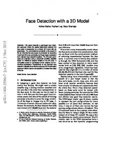
Figure II.1: A single frame of video from the IR Marks dataset. Before video collection, the subject’s face was marked using an infrared marking pen. The figure shows the same frame of video simultaneously captured by a visible-light camera (upper left) and three infrared-sensitive cameras. The infrared marks are clearly visible using the infrared cameras, but are not visible in the image from the visible-light camera.

23 collection process would make it impossible to measure a system’s performance on video of an unmarked face. In order for the field to continue to progress, there is a great need for publicly available data sets with ground truth information about the true 3D locations of the facial features that are to be tracked. Such data sets will facilitate refinement of one’s own algorithm during development, as well as provide standards for performance comparison with other systems. We have developed a new method for collecting the true 3D positions of points on smooth facial features (such as points on the skin) without leaving a visible trace in the video being measured. We used this technique, described in Section II.7 and Appendix II.A, to collect a face motion data set, the IR Marks video data set, which we are making available in order to begin filling the need for good data sets in the field. Figure II.1 shows an example of the same frame of video from the IR Marks data set, captured simultaneously by a visible-light camera and three infrared-sensitive cameras. We present our tracking results on this new data set in Section II.8, using it to compare our performance with other tracking systems and to measure the effects that changing parameter values have on system performance.

II.2

Background: Optic flow Let yt represent the current image (video frame) in an image sequence, and let lt

represent the 2D translation of an object vertex, x, at time t. We let x(lt ) represent the image location of the pixel that is rendered by vertex x at time t. We label all of the pixels in a neighborhood around vertex x by their 2D displacement, d, from x; viz. def

xd (lt ) = x(lt ) + d. The goal of the standard Lucas-Kanade optic flow algorithm [Lucas and Kanade, 1981; Baker and Matthews, 2002] is to estimate lt , the translation of the vertex at time t, given lt−1 , its translation in the previous image. All pixels in a neighborhood around x are constrained to have the exact same translation as x. The Lucas-Kanade algorithm uses the Gauss-Newton method (see Appendix II.C) to find the value of the translation, lt , that minimizes the squared image intensity difference between the image patch around

24 x in the current frame and the image patch around x in the previous frame: ˆlt = argmin 1 2 lt

X



2 yt xd (lt ) − yt−1 xd (lt−1 )

(II.1)

d∈D

where D is the set of displacements that defines the neighborhood (image patch) around a vertex. Constrained Optic Flow for Deformable 3D Objects

Under the assumption that

every vertex moves independently of the others, we would perform the minimization (II.1) separately for each vertex x. Suppose, however, that the vertices do not move independently, but rather move in concert according to a global model, as a function of pose parameters ut . In G-flow, for example, we constrain the locations of the object vertices on the image plane to be consistent with an underlying 3D morphable model. In our model, the pose ut comprises both the rigid position parameters (3D rotation and translation) and the nonrigid motion parameters (e.g., facial expressions) of the morphable model (see Section II.3.1 for details). Then the image location of the ith vertex is parameterized by ut : we let xi (ut ) represent the image location of the pixel that is rendered by the ith object vertex when the object assumes pose ut . Suppose that we know ut−1 , the pose at time t − 1, and we want to find ut , the pose at time t. This problem can be solved by minimizing the following form with respect to ut : n

2 1 X u ˆt = argmin yt xi (ut ) − yt−1 xi (ut−1 ) . 2 ut

(II.2)

i=1

Applying the Gauss-Newton method (see Appendix II.C) to achieve this minimization yields an efficient algorithm that we call constrained optic flow, because the vertex locations in the image are constrained by a global model. This algorithm, derived in Appendix II.D, is essentially equivalent to the methods presented in [Torresani et al., 2001; Brand, 2001]. In the special case in which the xi (ut ) are neighboring points that move with the same 2D displacement, constrained optic flow reduces to the standard Lucas-Kanade optic flow algorithm for minimizing (II.1). Standard optic flow (whether constrained or not) does not maintain a representation of uncertainty: for each new frame of video, it chooses the best matching pose,

25 throwing away all the rest of the information about the pose of the object, such as the degree of uncertainty in each direction. For example, optic flow can give very precise estimates of the motion of an object in the direction perpendicular to an edge, but uncertain estimates of the motion parallel to the edge, a phenomenon known in the psychophysics literature as the aperture problem. For our G-flow model, a key step in the inference algorithm is a Gauss-Newton minimization over pose parameters (described in Section II.5.2) that is quite similar to constrained optic flow. Unlike standard approaches to optic flow, however, our algorithm maintains an estimate of the entire probability distribution over pose, not just the peak of that distribution.

II.3

The Generative Model for G-Flow The problem of recovering 3D structure from sequences of 2D images has proven

to be a difficult task. It is an ill-posed problem, in that a given 2D image may be consistent with more than one 3D explanation. We take an indirect approach to the problem of inferring the 3D world from a 2D observation. We start with a model of the reverse process, which is much better understood: how 2D images are generated by a known 3D world. This allows us to frame the much harder problem of going from 2D images to 3D structure as Bayesian inference on our generative model. The Bayesian approach is well suited to this ill-posed problem, because it enables us to measure the relative goodness of multiple solutions and update these estimates over time. In this section, we lay out the forward model: how a 3D deformable object generates a video sequence (a sequence of 2D images). Then in Section II.5, we describe how to use Bayesian inference to tackle the inverse problem: Determining the pose (nonrigid and rigid motion) of the 3D object from an image sequence. Assumptions of the Model

We assume the following knowledge primitives:

• Objects occlude backgrounds. • Object texture and background texture are independent.

26 • The 3D geometry of the deformable object to be tracked is known in advance. In Chapter III, we will address how such 3D geometry could be learned using a neurally plausible architecture. In addition, we assume that at the time of object tracking, the system has had sufficient experience with the world to have good estimates of the following processes (it would be a natural extension to infer them dynamically during the tracking process): • Observation noise: the amount of uncertainty when rendering a pixel from a given texture value. • A model for pose dynamics • The texture process noise: How quickly each texel (texture element) of the foreground and background appearance models varies over time Finally, the following values are left as unknowns and inferred by the tracking algorithm: • Object texture (grayscale appearance) • Background texture • Rigid pose: Object orientation and translation • Nonrigid pose: Object deformation (e.g., facial expression)

II.3.1

Modeling 3D deformable objects In a 3D Morphable Model [Blanz and Vetter, 1999], we define a non-rigid object

by the 3D locations of n vertices. The object is a linear combination of k fixed morph bases, with coefficients c = [c1 , c2 , · · · , ck ]T . The fixed 3 × k matrix hi contains the position of the ith vertex in all k morph bases. Thus in 3D object-centered coordinates, the location of the ith vertex is hi c. Scale changes are accomplished by multiplying all k morph coefficients by the same scalar. In practice, the first morph basis is often the mean shape, and the other k − 1 morph bases are deformations of that base shape (e.g., the results of applying principal component analysis (PCA) to the 3D locations of the vertices in several key frames). In this case, the

27 first morph coefficient, c1 , can be used as a measure of scale. The transformation from object-centered to image coordinates consists of a rotation, weak perspective projection, and translation. Thus xi , the 2D location of the ith vertex on the image plane, is xi = grhi c + l, where r is the 3 × 3 rotation matrix, l is the 2 × 1 translation vector, and g =

(II.3) 1 0 0 010

is

the projection matrix. The object pose at time t, denoted by ut , comprises both the rigid motion parameters (rotation, r, and translation, l) and the nonrigid motion parameters (the morph coefficients, c): ut = {rt , lt , ct }. Note that while we always include the time subscript for the pose parameter, ut , to avoid clutter we usually omit the subscript t from its three components: ut = {r, l, c}.

II.3.2

(II.4)

Modeling an image sequence We model the image sequence Y as a stochastic process generated by three hidden

causes, U , V , and B, as shown in the graphical model (Figure II.3). The m × 1 random vector Yt represents the m-pixel image at time t. The n × 1 random vector Vt represents the n-texel object texture∗ , and the m × 1 random vector Bt represents the m-texel background texture. As illustrated in Figure II.2, the object pose, Ut , determines onto which image pixels the object and background texels project at time t. For the purposes of the derivations in this chapter, we make the following simplifying assumption. We assume that the object has n vertices, one corresponding to each texel in the object texture map, vt : the ith texel in vt corresponds to the ith vertex of the object. We further assume that the mapping (which is a function of the pose, ut ) from object texels (in vt ) to image locations (in yt ) is one-to-one, i.e., that every object texel renders exactly one pixel in the image (unless an object texel is self-occluded, in which case it does not render any image pixels). Thus, of the m pixels in each observed image, at most n of the pixels are rendered by the object (one pixel per unoccluded texel in vt ), and the remaining pixels in the image are rendered by the background. In ∗

We use the term texel (short for texture element) to refer to each individual element in a texture map, just as pixel (picture element) refers to an individual element of an image.

28

Bt

Vt

a(Ut ) Assigns texels to pixels

Yt

Figure II.2: Each pixel in image Yt is rendered using the color of either an object texel (a pixel in the object texture map, Vt ) or a background texel (a pixel in the background texture map, Bt ). The projection function a(Ut ), where Ut is the pose at time t, determines which texel is responsible for rendering each image pixel. practice, we actually use a great deal fewer vertices than pixels, and each pixel that is part of the object is rendered by interpolating the location from the surrounding vertex positions and correspondingly interpolating the texture value from the object texture map. However, the simplifying assumption that the rendering process is a one-to-one discrete function from vertices/texels to pixels is a convenient fiction, in that it makes the derivations easier to follow without affecting the underlying mathematics. The ith texel in the object texture map renders the pixel at xi (ut ), which is the image location to which vertex i projects. From Section II.3.1, this image location is given by: xi (ut ) = grhi c + l.

(II.5)

To simplify notation, we index pixels in the image vector, yt , by their 2D image locations.
Thus yt xi (ut ) represents the grayscale value of the image pixel that is rendered by object vertex i. In our image generation model, this is equal to the grayscale value of

29

3D Object Pose and Morph

U1 Object Texture

V1 B1

2D Background Texture

σw

Ut

Ut−1 Vt−1 Bt−1

Ψb

σw

σw

σw

Y1

Vt

Ψv

Bt

σw σw

Yt−1

Yt

Image Sequence

Observed 2D Image

Figure II.3: G-flow video generation model: At time t, the object’s 3D pose, Ut , is used to project the object texture, Vt , into the 2D image. This projection is combined with the background texture, Bt , to generate the observed image, Yt . The goal is to make inferences about (Ut , Vt , Bt ) based on the observed video sequence, {Y1 , . . . , Yt }. texel i in the object texture map, plus Gaussian observation noise: Foreground pixel xi (ut )



: Yt xi (ut ) = Vt (i) + Wt xi (ut ) ,


Wt xi (ut ) ∼ N (0, σw ),

σw > 0 (II.6)

where the random variables Wt (j) represent the independent, identically distributed observation noise (rendering noise) at every image pixel j ∈ {1, . . . , m}. The background texture map, bt , is the same size as the image yt . Every image pixel j that is not rendered by a foreground texel, is rendered by background texel j. The grayscale value of each pixel rendered by the background is equal to the grayscale value of the corresponding texel in the background texture map, plus Gaussian observation noise: Background pixel j

: Yt (j) = Bt (j) + Wt (j),

Wt (j) ∼ N (0, σw ),

σw > 0.

(II.7)

30 In order to combine the scalar equations (II.6) and (II.7) into a single vector equation, we introduce the projection function, a(Ut ). For a given pose, ut , the projection a(ut ) is a block matrix, def

a(ut ) =

h

av (ut )

ab (ut )

i

.

(II.8)

Here av (ut ), the object projection function, is an m×n matrix of 0s and 1s that tells onto which image pixel each object vertex projects; e.g., a 1 at row j, column i means that the ith object vertex projects onto image pixel j. Matrix ab (ut ), an m×m diagonal matrix of 0s and 1s, plays the same role for background pixels. Assuming the foreground mapping is one-to-one (each texel projects to exactly one pixel), we let ab (ut ) = Im −av (ut )[av (ut )]T , expressing the simple occlusion constraint that every image pixel is rendered by object or background, but not both. Then we can express the observation model given in (II.6) and (II.7) by a single matrix equation: 



Vt Yt = a(Ut )   + Wt Bt

Wt ∼ N (0, σw Im ),

σw > 0

(II.9)

where σw > 0 is a scalar. For t ≥ 2, the system dynamics are given by: v Vt = Vt−1 + Zt−1

v Zt−1 ∼ N (0, Ψv ),

Ψv is diagonal

b Bt = Bt−1 + Zt−1

b Zt−1 ∼ N (0, Ψb ),

Ψb is diagonal

(II.10)

where Z v , Z b , W are independent over time and of each other, and are independent of the initial conditions. The n values on the diagonal of ψv represent the variance of the process noise for each of the n texels of the object texture map. Similarly, the m values on the diagonal of ψb represent the variance of the process noise for the m background texels. We let the pose, Ut , be a Markov process with a known pose transition distribution: p(ut | u1:t−1 , y1:t−1 ) = p(ut | ut−1 ).

(II.11)

The form of the pose distribution is left unspecified since the algorithm proposed here does not require the pose distribution or the pose dynamics to be Gaussian. The model is specified by the following terms:

31 • Initial conditions, which consist of a distribution for the object pose U1 , and Gaussian distributions of object and background texture, V1 and B1 , all of which are independent of each other. We assume that the covariance matrix of V1 is diagonal (the initial noise on every foreground texel is independent of the noise on every other foreground texel) and the covariance matrix of B1 is a scalar times the identity matrix (the initial noise on every background texel is independent of, and has the same covariance as, the noise on every other background texel). • The diagonal covariance matrices for the state transitions (process noise), Ψv and Ψb . • The pose transition distribution, p(ut | ut−1 ). 2 I , where σ is a • The covariance matrix for the image rendering noise, Ψw = σw m w

scalar. Using standard methods, the above parameters could be either learned from training data, or inferred dynamically during tracking to adjust to the observed data. For the results described in this chapter, we simply choose generic parameter values that work well. For example, we use a weak model for the pose transition distribution p(ut | ut−1 ), that simply requires object pose to not change too much in adjacent frames, and also penalizes facial expressions whose morph coefficients exceed the range observed in the training data. The imaging model (e.g., weak perspective projection) determines the functions av and ab .

II.4 II.4.1

Inference in G-Flow: Preliminaries Conditionally Gaussian processes Nonrigid 3D tracking is a difficult nonlinear filtering problem because the image

location of each vertex is a nonlinear function of the pose (i.e., xi (ut ) and a(ut ) are nonlinear functions of ut ), and the image intensity is a nonlinear function of image location (i.e., yt (x) is a nonlinear function of x). Fortunately, the problem has a rich structure that we can exploit: under the G-flow model, video generation is a conditionally

32 Gaussian process [Chen et al., 1989; Doucet et al., 2000a; Chen and Liu, 2000; Doucet and Andrieu, 2002]. If the specific values taken by the pose sequence, u1:t , were known, then the texture processes, V and B, and the image process, Y , would be jointly Gaussian. In addition to V and B, the image sequence Y would itself be a linear Gaussian process, with time-varying parameter a(ut ) determined by the known pose ut . Hence, given the poses u1:t , we could use a Kalman filter to optimally infer the object and background texture maps from the observed images over time.

II.4.2

Importance sampling Importance sampling is a Monte Carlo technique that was designed in the 1940s

for efficient estimation of expected values [Doucet et al., 2000b]. The approach works as follows. Suppose we want to estimate the expected value of a function h of a random variable X, whose probability density function is p(x): Z
E h(X) = p(x)h(x)dx

(II.12)

One way to do so is to take n samples {x(1) , · · · , x(n) } from X and average the values taken by h on those samples n
1X h(x(i) ) E h(X) ≈ n

(II.13)

i=1

Instead of sampling directly from p, which may be intractable or computationally costly, in some cases it is desirable to obtain samples from a proposal distribution, π, from which samples can be drawn efficiently, and compensate by using importance weights that are proportional to the ratio of p to π. To see why, note that Z Z Z
p(x) h(x)dx = π(x)w(x)h(x)dx E h(X) = px (x)h(x)dx = π(x) π(x)

(II.14)

where the importance weight, w(x), is the ratio of the values taken by the desired distribution and the proposal distribution: w(x) =

p(x) . π(x)

(II.15)

33 Thus, the corresponding importance sampling estimate would be n
1X E h(X) ≈ w(x(i) )h(x(i) ) n

(II.16)

i=1

where now the samples {x(1) , · · · , x(n) } are taken from the proposal distribution π. Since the approach provides estimates for expected values of arbitrary functions h, it can be interpreted as providing an estimate for the distribution of X itself, i.e., pˆ(x) =

1 w(x)δ(x − x(i) ), n

(II.17)

where δ(·) is the Dirac delta function. When p(x) is only known up to a proportionality constant, then the importance weights are also known up to a proportionality constant. In this case we can rewrite (II.16) as follows: R E(X) = where w(x) ∝

p(x) π(x)

π(x)w(x)h(x)dx R π(x)w(x)dx

(II.18)

is now known up to a normalizing constant. Since the ratio of two

consistent estimators is also consistent, a standard estimate in this case is as follows [Andrieu et al., 2003]:
E h(X) ≈ where

1 n

Pn n (i) (i) X i=1 w(x )h(x ) = w(x ˜ (i) )h(x(i) ), P n 1 (i) ) w(x i=1 n i=1 w(x(i) ) w(x ˜ (i) ) = Pn (j) j=1 w(x )

(II.19)

(II.20)

is the normalized importance weight. The corresponding estimate of the distribution of X is as follows: pˆ(x) = w(x)δ(x ˜ − x(i) ).

(II.21)

For the estimation process to be efficient, the proposal distribution π must be as close as possible to the original distribution, p. For our application, we found that in addition to Rao-Blackwellization, it was critical to use the Gauss-Newton method and Laplace’s method to generate good proposal distributions for importance sampling. As we explain in Section II.5.2.1, we accomplish this in the context of G-flow by performing an optic flow-like optimization.

34

II.4.3

Rao-Blackwellized particle filtering Stochastic filtering is the process of sequentially estimating the distributions of a

random process (a sequence of random variables), obtaining each new estimate by combining one’s prior estimates with the current observation. In linear Gaussian dynamical systems, inference (stochastic filtering) can be performed exactly, using a Kalman filter [Kalman, 1960]. For nonlinear problems, it is standard to use approximations, such as an extended Kalman filter, variational methods, and Monte Carlo (sampling-based) methods such as particle filters. In the particle filtering literature, the term Rao-Blackwellization [Doucet et al., 2000a; Doucet and Andrieu, 2002] refers to some dimensions of the system’s state being integrated out analytically. As a result, the portion of the system’s state that must be sampled (that must be represented using particles) is lower dimensional. Thus the variance of the Rao-Blackwellized particle filter is reduced, and fewer samples of the state space (fewer particles) are required in order to achieve the same level of performance. The Rao-Blackwellized particle filtering approach, also known in the statistics community as a Monte Carlo filtering solution for conditionally Gaussian processes [Chen et al., 1989; Chen and Liu, 2000], takes advantage of the structure of the filtering distribution in order to get the best of both worlds: it uses exact filtering on the variables that can be inferred analytically, and uses the Monte Carlo approach of particle filtering only for the variables that cannot be inferred exactly. Standard particle filtering alone is insufficient to solve the 3D nonrigid tracking problem, because the combined sample space for pose and texture would be too highdimensional to sample effectively. In order to perform stochastic filtering on the G-flow model, we use a Rao-Blackwellized particle filter, employing a particle filter to estimate the pose distribution, and using an exact solution to infer the texture appearance given the pose. We use particle filtering to obtain a distribution of pose experts: Each expert corresponds to a particular pose history, u1:t , and the entire collection of experts is our Monte Carlo estimate of the pose distribution. For each expert, we then use exact filtering (the Kalman filtering equations) to infer the distribution of texture given the sampled pose distribution.

35

II.5

Inference in G-flow: A bank of expert filters Our goal is to find an expression for p(ut , vt , bt | y1:t ), the posterior distribution of

pose and texture given the observed sequence of images . This is commonly known as the filtering distribution. In addition, we want the filtering distribution to be updated in a recursive manner; i.e., given the filtering distribution from time t − 1 and given a new image yt at time t, we want to find the filtering distribution at time t, without requiring knowledge of the past images. The following equation provides the key to doing so. Using the law of total probability, we have that Z p(ut , vt , bt | y1:t ) = p(ut , vt , bt , u1:t−1 | y1:t )du1:t−1 Z = p(u1:t−1 | y1:t )p(ut , vt , bt | u1:t−1 , y1:t )du1:t−1 , or equivalently: Z p(ut , vt , bt | y1:t ) = {z } |

p(u1:t−1 | y1:t ) p(ut | u1:t−1 , y1:t ) p(vt , bt | u1:t , y1:t ) du1:t−1 (II.22) | {z } | {z } | {z }

Filtering Distribution

Credibility of expert

Pose Opinion Texture Opinion of expert of expert (Distribution of texture given pose)

We can think of the integral in (II.22) as a weighted sum over a distribution of experts, where each expert corresponds to a past history of poses, u1:t−1 . Each expert is endowed with: (1) an opinion distribution about the current pose, p(ut | u1:t−1 , y1:t ); (2) an opinion distribution about the current object and background textures, p(vt , bt | u1:t , y1:t ); and (3) a credibility value, p(u1:t−1 | y1:t ). Because the image generation model is conditionally Gaussian given the pose (see Section II.4.1), we can perform exact inference to determine the foreground and background texture opinion distributions for each pose expert. This turns out to be a filtering problem for each expert; thus, inference in G-flow is performed using a bank of expert filters. We adopt the following scheme: Use Monte-Carlo methods to obtain a distribution of pose experts (highly probable samples of U1:t ), then use analytic methods to determine the exact filtering distribution of texture, V1:t , B1:t , for each expert. Table II.1 gives an overview of how we compute each term in the integral. We cover pose opinion in II.5.2,

36 texture opinion (the distribution of texture given pose) in Section II.5.1, and credibility in II.5.3. Table II.1: Overview of Inference in G-flow. To infer the filtering distribution at time t, we evaluate the integral in (II.22) as a sum over experts. For every expert, we compute each of the three terms in the integral using the method indicated. −→

Efficient Monte Carlo sampling. We use importance sampling, starting with a Gaussian proposal distribution for importance sampling that is obtained by Laplace’s method under the assumption of a white-noise background.

Texture opinion −→ (Section II.5.1)

Analytical solution given the estimated pose opinion distribution (object and background dynamic texture maps for each expert).

−→

Analytical solution given the estimated pose opinion distribution.

Pose opinion (Section II.5.2)

Credibility (Section II.5.3)

II.5.1

Expert Texture Opinions Due to the conditionally Gaussian nature of the image generation process, the

distribution of texture given a pose sequence, u1:t , and a sequence of images, y1:t , is Gaussian. The mean of this texture opinion, which can be thought of as an expert’s texture template, consists of a single texture value for each texel (each location in the texture map). The covariance matrix of the texture opinion, which in our model can be shown to be diagonal, represents the expert’s uncertainty about the texture values at each texel in the texture maps. The problem of updating the texture mean and texture uncertainty maps given a sequence of poses, is equivalent to solving a time-dependent Kalman filtering problem, for which well known recursive solutions exist. Let us denote the expected values and covariance matrices of the texture maps

37 (the texel means and variances) as follows: def

vˆt|t (i) = ith element of E(Vt | u1:t , y1:t ), def

vˆt|t−1 (i) = ith element of E(Vt | u1:t−1 , y1:t−1 ), ˆbt|t (j) def = j th element of E(Bt | u1:t , y1:t ), ˆbt|t−1 (j) def = j th element of E(Bt | u1:t−1 , y1:t−1 ) .

(II.23)

def

Vt|t (i) = ith diagonal element of V ar(Vt | u1:t , y1:t ), def

Vt|t−1 (i) = ith diagonal element of V ar(Vt | u1:t−1 , y1:t−1 ), def

Bt|t (j) = j th diagonal element of V ar(Bt | u1:t , y1:t ),

(II.24)

def

Bt|t−1 (j) = j th diagonal element of V ar(Bt | u1:t−1 , y1:t−1 ). We refer similarly to the process noise for each texel: def

Ψv (i) = ith diagonal element of Ψv

def

Ψb (j) = j th diagonal element of Ψb . (II.25)

II.5.1.1

Kalman equations for dynamic update of texel maps

Assume that by time t, the system already has the means and variances of the predictive texture maps from the previous time step: {ˆ vt|t−1 , ˆbt|t−1 , Vt|t−1 , Bt|t−1 }. First we apply the Kalman state estimation (correction) equations to obtain the sufficient statistics of the filtering distribution for texture at time t: {ˆ vt|t , ˆbt|t , Vt|t , Bt|t }. From these, we apply the Kalman state propagation (prediction) equations to obtain the predictive distribution at time t: {ˆ vt+1|t , ˆbt+1|t , Vt+1|t , Bt+1|t }.

Correction equations :


  vˆt|t (i) = k t (i) yt xi (ut ) + 1 − k t (i) vˆt|t−1 (i)

(II.26)

Vt|t (i) = [1 − k t (i)] Vt|t−1 (i)

(II.27)

38 where k t (i), the Kalman gain for texel i, is the scalar given by:  Vt|t−1 (i)    , if texel i is visible (II.28) k t (i) = Vt|t−1 (i) + σw    0, if texel i is occluded. Prediction equations :

vˆt+1|t (i) = vˆt|t (i)
  = k t (i) yt xi (ut ) + 1 − k t (i) vˆt|t−1 (i)

(II.29)

Vt+1|t (i) = Vt|t (i) + Ψv (i) = [1 − k t (i)] Vt|t−1 (i) + Ψv (i)

(II.30)

Identical update equations are obtained for the update of background maps, but replacing the object texture means and variances by the corresponding background texture means and variances (see Appendix II.E). II.5.1.2

Interpreting the Kalman equations

The updated texture map is a combination of the previous texture map and the new image. The Kalman gain dynamically determines the relative contributions of the previous texture map and the new image. A Kalman gain of 1 means that all of the information comes from the new observation, and the previous texture map is ignored. On the other hand, a Kalman gain of 0 means that all of the information comes from the previous texture map, and the new image is ignored. It follows from (II.28) that if the uncertainty (variance) of a texel in the object texture map is much larger than the image rendering noise, then the Kalman gain will be close to 1: Vt|t−1 (i)  σw

=⇒

k t (i) ≈ 1.

(II.31)

In other words, the information from the texture map will be ignored in favor of the (more accurate) information from the image. On the other hand, if a texel’s variance is much less than the image rendering noise, then the Kalman gain will be close to 0: Vt|t−1 (i)  σw

=⇒

k t (i) ≈ 0,

(II.32)

and thus the information from the image will be ignored in favor of the (more accurate) information from the texture map.

39

II.5.2

Expert Pose opinions Our goal is to find an expression for the pose opinion p(ut | u1:t−1 , y1:t ),

(II.33)

the belief of expert u1:t−1 about the pose at time t. Since the effect of ut on the observed image yt is nonlinear, exact analytical solutions are not available. However, the spatiotemporal smoothness of video signals can be exploited to obtain efficient estimates: First approximate the pose opinion of each expert as a Gaussian distribution, then use importance sampling to correct for the potential bias introduced by the Gaussian approximation. II.5.2.1

Gaussian approximation of each expert’s pose opinion

Laplace’s method consist of approximating an arbitrary probability density function (pdf) by a Gaussian function centered at the peak of the distribution and with covariance matrix proportional to the inverse of the matrix of second-order derivatives (the Hessian matrix) at the peak. This is equivalent to approximating the logarithm of the pdf with a second-order Taylor series approximation centered about the peak of the distribution. We apply Laplace’s method to obtain a Gaussian approximation to the pose opinion distribution of each expert. We then use this Gaussian approximation as our proposal distribution for importance sampling. The method requires: (1) Finding the peak of the distribution, and (2) estimating the spread of the opinon (i.e., the Hessian matrix) at the peak. Finding the Peak of an Expert’s Pose Opinion

We want to estimate u ˆt (u1:t−1 ),

the value of ut that maximizes the pose opinion (II.33). We can write the pose opinion

40 distribution as: p(ut | u1:t−1 , y1:t ) | {z } Pose Opinion of expert u1:t−1

=

p(ut | u1:t−1 )p(y1:t | u1:t ) p(y1:t | u1:t−1 )

=

p(ut | u1:t−1 ) p(y1:t−1 | u1:t ) p(yt | u1:t , y1:t−1 ) p(y1:t | u1:t−1 )

=

p(y1:t−1 | u1:t−1 ) p(ut | ut−1 ) p(yt | u1:t , y1:t−1 ). p(y1:t | u1:t−1 )

(II.34)

To find the peak of this pose opinion distribution, we maximize (II.34) with respect to ut , eliminating the terms that are constant with respect to ut : def

u ˆt (u1:t−1 ) = argmax p(ut | u1:t−1 , y1:t ) ut

= argmax p(ut | ut−1 ) p(yt | u1:t , y1:t−1 ).

(II.35)

ut

We now need an expression for the final term in (II.35), the predictive distribution p(yt | u1:t , y1:t−1 ). As we derive in Appendix II.F (II.178), m log 2π (II.36) 2 " # n
[yt (xi (ut )) − vˆt|t−1 (i)]2 1X − log Vt|t−1 (i) + σw + 2 Vt|t−1 (i) + σw i=1 " #
[yt (j) − ˆbt|t−1 (j)]2 1 X log Bt|t−1 (j) + σw + , − 2 Bt|t−1 (j) + σw

log p(yt | u1:t , y1:t−1 ) = −

j6∈X (ut )

where xi (ut ) is the image pixel rendered by the ith object vertex when the object assumes pose ut , and X (ut ) is the set of all image pixels rendered by the object under pose ut . The first sum in (II.36) corresponds to the foreground pixels, while the second sum in (II.36) corresponds to the background pixels. As we show in Appendix II.F, substituting (II.36) into (II.35) and eliminating the

41 terms that don’t depend on ut yields: u ˆt (u1:t−1 ) = argmin − log p(ut | ut−1 )

(II.37)

ut

Foreground terms z }| { n  vt|t−1(i)]2 1X [yt (xi (ut )) −ˆ +log[Vt|t−1 (xi (ut )) + σw ] + 2 Vt|t−1 (i) + σw i=1

! [yt (xi (ut )) −ˆbt|t−1(xi (ut ))]2 − −log[Bt|t−1 (xi (ut )) + σw ] Bt|t−1(xi (ut )) +σw | {z } Background terms The sum in (II.37) is difficult to optimize in the general case. However, an efficient approximation can be obtained under the following assumptions: (1) If there are no selfocclusions (i.e., the object texels are never occluded), then the second foreground term, log[Vt|t−1 (xi (ut )) + σw ], is constant with respect to pose, and thus may be ignored in the optimization. (2) If the uncertainty about the background is very large, e.g., a white noise background model, then the background terms can be ignored. (3) If the transition probability is Gaussian, then the prior term, log p(ut | ut−1 ), becomes a quadratic penalty term. Under these conditions, the optimization problem reduces to solving a nonlinear regression problem, for which the Gauss-Newton algorithm is an efficient and popular approach. The details of this method for estimating the peak of the pose opinion are explained in Appendix II.G. (d)

We index each individual expert by d, where d ∈ {1, 2, . . . , η}. Then u1:t−1 refers (d)

to the pose history of expert d, and u ˆt (u1:t−1 ) refers to our estimate of the peak of that expert’s pose opinion, obtained (as explained above) by using Gauss-Newton to minimize (II.37). Estimating the Spread of the Expert’s Pose Opinion estimate

(d) u ˆt (u1:t−1 ),

We have just seen how to

the peak of the pose opinion of expert d. The Laplace estimate of

the covariance matrix of this expert’s pose opinion is the inverse of the Hessian matrix (matrix of second derivatives) of (II.37) evaluated at this peak, under the same assumptions listed above for obtaining the peak. (A full derivation is in Appendix II.H.) We
(d) call this Laplace estimate U u ˆt (u1:t−1 ) .

42 The Laplace estimate of the pose opinion of expert d is a Gaussian distribution
(d) (d) whose mean is u ˆt (u1:t−1 ) and whose covariance is proportional to U u ˆt (u1:t−1 ) : 
 def (d) (d) (d) π(ut | u1:t−1 , y1:t ) = N u ˆt (u1:t−1 ), α U u ˆt (u1:t−1 ) . (II.38) The parameter α > 0 determines the sharpness of the distribution. (Note that letting α → 0 would be equivalent to the greedy approach of simply setting the new pose ut equal to the peak of the estimated pose opinion distribution.) II.5.2.2

Importance sampling correction of the Gaussian approximation (d)

Let u1:t−1 represent the dth pose expert. Instead of simply accepting the Gaussian approximation (II.38) to the opinion distribution of that expert, we use it as a proposal distribution for importance sampling. This corrects for the potential bias induced by the Gaussian approximation and guarantees that we have a consistent estimator for the opinion distribution of that expert. (d)

For each expert u1:t−1 , we begin by generating a set of λ independent samples (d,1)

{ut

(d,λ)

, . . . , ut

(d)

} drawn from the proposal distribution π(ut | u1:t−1 , y1:t ). We then as-

sign each of these samples from the proposal distribution an importance weight, wt (d, e), which is proportional to the ratio between the true pose opinion distribution and the proposal distribution, both evaluated at that sample: wt (d, e) ∝

(d,e)

| u1:t−1 , y1:t )

(d,e)

| u1:t−1 , y1:t )

p(ut

π(ut

(d)

(d)

.

(II.39)

We may choose the proportionality constant in order to simplify the evaluation of (II.39). Observing that the pose opinion of expert d is proportional to the joint distribution over the current pose and image, given the pose and image history, (d)

(d)

p(ut | u1:t−1 , y1:t ) =

p(yt , ut | u1:t−1 , y1:t−1 ) (d) p(yt | u1:t−1 , y1:t−1 )

(d)

∝ p(yt , ut | u1:t−1 , y1:t−1 ),

(II.40)

we let wt (d, e) =

(d,e)

| u1:t−1 , y1:t−1

(d,e)

| u1:t−1 , y1:t )

p yt , ut π(ut

(d,e)

=

p(ut

(d)


(II.41)

(d)

(d)

(d)

(d,e)

| ut−1 ) p(yt | u1:t−1 , ut (d,e)

π(ut

(d)

| u1:t−1 , y1:t )

, y1:t−1 )

,

(II.42)

43 and the normalized importance weights are: wt (d, e) . w ˜t (d, e) = Pλ f =1 wt (d, f )

(II.43)

Equation (II.42) is used to compute the importance weights: The pose transition proba(d,e)

bility in the numerator, p(ut

(d)

| ut−1 ), is known (as part of the image generation model).

The predictive probability in the numerator is expressed in (II.36), and the proposal probability in the denominator is expressed in (II.38). Our importance sampling estimate of the expert’s pose opinion distribution is as follows: (d)

(d,e)


pˆ(ut | u1:t−1 , y1:t ) = δ ut − ut

II.5.3

w ˜t (d, e).

(II.44)

Expert credibility At the beginning of frame t, each expert d has a posterior credibility from the (d)

previous frame, p(u1:t−1 | y1:t−1 ), which our system represents by (d)

(d)

Ct−1|t−1 = pˆ(u1:t−1 | y1:t−1 ),

(II.45)

a consistent estimate of the credibility before the image at time t is observed. The (d)

credibility of expert d at time t, the scalar p(u1:t−1 | y1:t ), is represented by (d)

(d)

Ct−1|t = pˆ(u1:t−1 | y1:t ),

(II.46)

a consistent estimate of the credibility of expert d after the new image, yt , has been observed. Suppose we have η opinion experts at time t, each endowed with a consistent (d)

(d)

estimate, Ct−1|t−1 = pˆ(u1:t−1 | y1:t−1 ), of its posterior credibility from the previous frame. After image yt is observed, the credibility can be updated using Bayes rule: (d) p(u1:t−1 | y1:t )

|

{z

Credibility of expert d

}

(d)

(d)

(d)

(d)

p(u1:t−1 | y1:t−1 ) p(yt | u1:t−1 , y1:t−1 ) = p(yt | y1:t−1 ) ∝ p(u1:t−1 | y1:t−1 ) p(yt | u1:t−1 , y1:t−1 )

(II.47)

44 (d,e)

We already generated a set of samples {ut

: e = 1, . . . , λ} to estimate the pose opinion

of the dth expert. We can now use these same samples to estimate the final term in (II.47). Note that Z

(d) p(yt | u1:t−1 , y1:t−1 )

(d)

p(yt , ut | u1:t−1 , y1:t−1 )dut

=

(d)

p(yt , ut | u1:t−1 , y1:t−1 )

Z = (d,e)

Since the samples ut

(d) π(ut | u1:t−1 , y1:t )

(d)

π(ut | u1:t−1 , y1:t ) dut

(II.48) (d)

were drawn from the proposal distribution π(ut | u1:t−1 , y1:t ), we

can use them to estimate the integral in (II.48): (d,e)

(d) pˆ(yt | u1:t−1 , y1:t−1 )

(d)

λ | u1:t−1 , y1:t−1 1 X p yt , ut = (d,e) (d) λ π(ut | u1:t−1 , y1:t ) e=1




λ

1X = wt (d, e), λ

(II.49)

e=1

where the last step follows from (II.41). Substituting (II.49) into (II.47), we obtain a consistent estimate for the credibility of the dth expert: (d)

(d)

(d)

Ct−1|t = pˆ(u1:t−1 | y1:t ) ∝ Ct−1|t−1

λ X

wt (d, e),

(II.50)

e=1

where we normalize so that the credibilities of all experts sum to 1: (d) Ct−1|t

(d,e)

Let u1:t

P (d) Ct−1|t−1 λe=1 wt (d, e) = P  (f )  Pλ f Ct−1|t−1 e=1 wt (f, e)

(II.51)

represent the concatenation of the pose history of expert d with pose (d,e)

sample e of the same expert: u1:t

def

(d)

(d,e)

= {u1:t−1 , ut

}. To compute the posterior credibil-

ities for frame t, note that (d,e)

(d)

(d,e)

p(u1:t | y1:t ) = p(u1:t−1 | y1:t ) p(ut

(d)

| u1:t−1 , y1:t )

(II.52)

Thus, a consistent estimator of the posterior credibilities at time t is: (d,e)

(d)

pˆ(u1:t | y1:t ) = Ct|t−1 w ˜t (d, e).

(II.53)

45

II.5.4

Combining Opinion and Credibility to estimate the new filtering distribution (d)

If there are η experts, u1:t−1 where d ∈ {1, . . . , η}, and each of these experts has (d,e)

λ pose samples, ut

where e ∈ {1, . . . , λ}, then there are a total of η · λ potential next-

generation pose experts, which we shall call seeds. Say the number of next-generation experts desired is ν. These are obtained by sampling ν times, with replacement, from (d,e)

the set of all η · λ seeds, where on each draw, the probability of choosing seed u1:t given by

(d,e) pˆ(u1:t | y1:t )

is

from (II.53).

After this resampling step, known in the literature as a selection step [Andrieu (d)

et al., 2003], the filtering distribution is represented by ν pose experts, u1:t where d ∈ {1, . . . , ν}, and each expert is assigned equal posterior credibility: (d)

Ct|t =

1 . ν

(II.54)

A consistent estimator of the filtering distribution for pose at time t is obtained by integrating over all of the next-generation experts, weighting each by its credibility: Z pˆ(ut | y1:t ) =

pˆ(u1:t | y1:t )d(u1:t−1 ) =

ν X

(d)
(d) Ct|t ,

δ ut − ut

(II.55)

d=1 (d)

where δ(·) is the Dirac delta function. For each new expert u1:t , the corresponding texture opinion is Gaussian and fully determined by its mean and variance, as explained in Section II.5.1. Thus the following is a joint estimator of the filtering distribution: the joint distribution of pose, object texture, and background texture, given the images up to time t: Z pˆ(ut , vt , bt | y1:t ) =

pˆ(u1:t , vt , bt | y1:t )d(u1:t−1 ) X (d) (d) = δ(ut − ut ) Ct|t N (vt ; vˆt|t , Vt|t ) N (bt ; ˆbt|t , Bt|t )

(II.56) (II.57)

d

II.5.5

Summary of the G-flow inference algorithm Here is a summary of the G-flow inference algorithm, which has been the subject of

this entire section (Section II.5). At each time step (each frame of video), the procedure is to first obtain the filtering distribution for pose (Step I), then find the distribution of

46 texture given those pose experts (Step II). As is common in particle filters, we do not resample at every time step [Arulampalam et al., 2002]. Rather, we resample periodically. We call time steps at which we resample resampling frames, and call the other time steps continuation frames. The instructions for finding the pose filtering distribution in continuation frames (Step IC) are a simpler, reduced version of the instructions for resampling frames (Step IB). I. Filtering distribution for pose At the end of each time step t, our estimate of the filtering distribution for pose is: pˆ(ut | y1:t ) =

η X

(d)

(d)

Ct|t δ(ut − ut ),

(II.58)

d=1

where η is the number of experts at time t. Thus the filtering distribution for pose (d)

at each frame, t, is determined by the poses of the η experts, {ut and the weight of each expert,

(d) wt .

: d = 1, · · · , η},

For the first video frame (t = 1), the filtering

distribution for pose is obtained using Step A below. Every subsequent video frame, t > 1, is either a resampling frame (use Step B) or a continuation frame (use Step C), with resampling frames occuring periodically. A. Initialization (t = 1) (d)

1. Obtain the pose of each of the η experts by sampling {u1 : d = 1, . . . , η} from p(u1 ). 2. Every expert at t = 1 has the same Gaussian predictive texture distributions for object and background, which are given as part of the model specification: For each expert d ∈ {1, . . . , η}, (d)

vˆ1|0 = vˆ1|0 ,

(d)

V1|0 = V1|0 ,

ˆb(d) = ˆb1|0 , 1|0

(d)

B1|0 = B1|0 .

(II.59)

3. Observe y1 , the first image in the video sequence. 4. To calculate the posterior credibility of the dth expert, use (II.36): (d)

(d)

C1|1 ∝ p(y1 | u1 ),

normalized so that

η X d=1

B. Resampling frames

(d)

C1|1 = 1.

(II.60)

47 1. Observe yt , the image at time t. 2. Use the Gauss-Newton method to estimate the peak of each expert’s (d)

pose opinion distribution, u ˆt (u1:t−1 ), as explained in Section II.5.2.1 and Appendix II.G. 3. For each expert d, use Laplace’s method to estimate the covariance of
(d) the expert’s pose opinion distribution about that peak, U u ˆt (u1:t−1 ) . (d,e)

= {r(d,e) , l(d,e) , c(d,e) },

Then generate a set of λ independent samples, ut

e ∈ {1, · · · , λ}, from the Gaussian proposal distribution: 
 def (d) (d) (d) π(ut | u1:t−1 , y1:t ) = N u ˆt (u1:t−1 ), α U u ˆt (u1:t−1 ) ,

(II.61)

as explained in Section II.5.2.1 and Appendix II.H. (d,e)

4. For each sample ut

, use (II.36) to calculate the value of the predic(d)

(d,e)

tive distribution, p(yt | u1:t−1 , ut

, y1:t−1 ). Use this value to obtain the

sample’s importance weight, wt (d, e): (d,e)

wt (d, e) =

p(ut

(d)

(d)

(d,e)

| ut−1 ) p(yt | u1:t−1 , ut (d,e)

π(ut

, y1:t−1 )

(d)

.

(II.62)

| u1:t−1 , y1:t ) (d)

(d)

5. Estimate the credibility of the dth expert, Ct−1|t = pˆ(u1:t−1 | y1:t ): (d)

(d)

Ct−1|t ∝ Ct−1|t−1

λ X

wt (d, e),

normalized so that

e=1

η X

(d)

Ct−1|t = 1.

d=1

(II.63) (j)

6. Create ν next-generation pose experts, {u1:t : j = 1, . . . , ν}, as follows. a. Randomly select a parent expert, d, who will sire the child. The probability of selecting parent expert d is equal to that parent’s credibility, (d)

Ct−1|t . (d,e)

b. Randomly select ut

, the child’s pose at time t, from the parent’s (d,1)

pose opinion (from the set of samples {ut ability of selecting pose

(d,e) ut

(d,2)

, ut

, . . .}). The prob-

is proportional to that sample’s impor-

tance weight, wt (d, e). c. The pose history for the new child (the next-generation expert) is:  (d) (j) (d,e) u1:t = u1:t−1 , ut .

(II.64)

48 7. Give every next-generation pose expert equal posterior credibility: (j)

Ct|t =

1 . ν

(II.65)

C. Continuation frames 1. Observe yt , the image at time t. 2. Use the Gauss-Newton method to estimate the peak of each expert’s (d)

pose opinion distribution, u ˆt (u1:t−1 ), as explained in Section II.5.2.1 and Appendix II.G, and assign that pose to the expert at time t: (d,1)

ut

(d)

=u ˆt (u1:t−1 ).

(II.66)

For each expert d, use (II.36) to calculate the value of the predictive (d)

(d,1)

distribution, p(yt | u1:t−1 , ut (d,1)

wt (d, 1) = p(ut

, y1:t−1 ). Use this value to obtain wt (d, 1):

(d)

(d)

(d,1)

| ut−1 )p(yt | u1:t−1 , ut

, y1:t−1 )

(d)

(II.67)

(d)

3. Estimate the credibility of the dth expert, Ct−1|t = pˆ(u1:t−1 | y1:t ): (d)

(d)

Ct−1|t ∝ Ct−1|t−1 wt (d, 1),

normalized so that

η X

(d)

Ct−1|t = 1. (II.68)

d=1

4. Each new expert’s pose history is a concatenation of the old expert’s pose history and its new pose at time t: (d)

(d)

(d,1)

u1:t = {u1:t−1 , ut

}.

(II.69)

5. Set the posterior credibility of each new expert equal to its credibility: (d)

(d)

Ct|t = Ct−1|t

(II.70)

II. Distribution of texture given pose For each new expert d, the Gaussian predictive distribution of texture given the (d)

pose history, u1:t , is obtained from the previous frame’s predictive distribution for

49 texture using the Kalman equations for each texel: object texel i :

where

 (d) (d) (d) (d)
 (d) vˆt+1|t (i) = k t (i) yt xi (ut ) + 1 − k t (i) vˆt|t−1 (i) (II.71)   (d) (d) (d) Vt+1|t (i) = 1 − k t (i) Vt|t−1 (i) + Ψv (i) (II.72)  (d) Vt|t−1 (i)     , if texel i is visible (d) (d) (II.73) k t (i) = Vt|t−1 (i) + σw     0, if texel i is occluded.

  ˆb(d) (j) = k (d) (j) yt (j) + 1 − k (d) (j) ˆb(d) (j) (II.74) t t t+1|t t|t−1   (d) (d) (d) Bt+1|t (j) = 1 − k t (j) Bt|t−1 (j) + Ψb (i) (II.75)  (d) Bt|t−1 (j)     (d) , if texel j is visible (d) where k t (j) = Bt|t−1 (j) + σw (II.76)     0, if texel j is occluded.

background texel j :

II.6

Relation to optic flow and template matching In basic template matching, the same time-invariant texture map is used to track

every frame in the video sequence. Optic flow can be thought of as template matching with a template that is completely reset at each frame for use in the subsequent frame. In most cases, optimal inference under G-flow involves a combination of optic flow-based and template-based tracking, in which the texture template gradually evolves as new images are presented. Pure optic flow and template-matching emerge as special cases.

II.6.1

Steady-state texel variances For texels that are never occluded, the Kalman filter asymptotically approaches a

steady state in which the texel variance is constant. To find V∞ (i) and k ∞ (i), the steadystate variance and steady-state Kalman gain of object texel i, we substitute into (II.30) and (II.28):   V∞ (i) = 1 − k ∞ (i) V∞ (i) + Ψv (i) k ∞ (i) =

V∞ (i) . V∞ (i) + σw

(II.77) (II.78)

50 Substituting (II.78) into (II.77) yields the algebraic Ricatti equation, V∞ (i) =

σw V∞ (i) + Ψv (i), V∞ (i) + σw

which we can solve for the steady-state texel variance, V∞ (i): p Ψv (i) + Ψ2v (i) + 4σw Ψv (i) V∞ (i) = . 2

(II.79)

(II.80)

We can then solve for the steady-state Kalman gain by substituting this value into (II.78): p −Ψv (i) + Ψ2v (i) + 4σw Ψv (i) k ∞ (i) = . (II.81) 2σw A useful descriptive parameter of the Kalman filters is τt (i), which we call the temperature of object texel i at time t, defined by: def

τt (i) = Vt|t−1 (i) + σw .

(II.82)

As we saw in (II.36), the temperature τt (i) is the variance of the predictive distribution for the intensity of the image pixel rendered by texel i. It is also the denominator of the foreground term in the G-flow objective function (II.37). We call it temperature in analogy to the role of the term temperature in statistical mechanics; it provides a measure of the total amount of noise in the texture value of each image pixel. A useful parameter for characterizing the Kalman filters is the steady-state temperature of texel i, denoted τ∞ (i): τ∞ (i) = V∞ (i) + σw .

II.6.2

(II.83)

Optic flow as a special case Suppose that the pose transition probability p(ut | ut−1 ) is uninformative, and that

the background is uninformative (e.g., a white noise background). Then the only terms remaining to minimize in the G-flow objective function (II.37) are the two foreground terms. If we further suppose that there are no self-occlusions (none of the object texels 
 is ever occluded), then the second foreground term, log Vt|t−1 xi (ut ) + σw , is constant with respect to pose, and thus may be ignored in the optimization. In this case, the only term remaining to minimize in the G-flow objective function (II.37) is the first

51 foreground term: u ˆt (u1:t−1 ) = argmin ut

n 1 X [yt (xi (ut )) − vˆt|t−1(i)]2 . 2 Vt|t−1 (i) + σw

(II.84)

i=1

Suppose we further restrict our model so that the process noise is the same at every texel and is much larger than the rendering noise, i.e., Ψv = σv In ,

where

σv  σw .

(II.85)

Once the system has settled to its steady state, it follows from the formula for steady-state texel variance (II.80) that every texel will have the same variance, V∞ ≈ σv , and it then follows from equation (II.78) that every texel’s Kalman gain will be k ∞ (i) ≈ 1. As a result, the Kalman equation for the object texture map means (II.29) reduces to:
vˆt|t−1 = yt−1 xi (ut−1 ) ,

(II.86)

i.e., the mean of texel i of the object texture map is simply the texture value taken from the location of vertex i in the previous image. Hence, the G-flow objective function (II.84) further reduces to u ˆt (u1:t−1 ) = argmin ut

n 2 1 X yt (xi (ut )) − yt−1 (xi (ut−1 )) , 2

(II.87)

i=1

which is identical to the constrained optic flow objective function (II.2). With this objective function, the Gauss-Newton minimization that we use to find the peak of the pose opinion (see Section II.5.2.1 and Appendix II.G) reduces to exactly the GaussNewton minimization performed in optic flow. Thus constrained optic flow [Torresani et al., 2001; Brand and Bhotika, 2001; Brand, 2001] is simply a special limiting case of optimal inference under G-flow, with a single expert (η = 1) and with sampling parameter α → 0. Interpretation

Assuming that the G-flow generative model is a fairly accurate model

of the world, we can conclude that optic flow is only optimal in the extreme conditions given by (II.85), which essentially amount to the object’s texture changing so fast that at every point on the object (at every vertex), the texture value varies a great deal from each frame to the next. However, optic flow is typically applied in situations in which the

52 object’s texture changes very little from each frame to the next. In such situations, the optimal solution calls not for optic flow, but for a texture map that integrates information across multiple frames.

II.6.3

Template Matching as a Special Case Suppose that the pose transition probability p(ut | ut−1 ) is uninformative, that the

background is uninformative, and that none of the foreground texels is ever occluded, as in the optic flow case above. Then the G-flow objective function (II.37) reduces to just its foreground term (II.84). In order for our system to reduce to template-matching with a fixed template, we need it to be the case that once the system reaches steady state, the texture map means do not change at all as new images are observed. In other words, we need the steady-state Kalman gain to be k ∞ (i) ≈ 0. To make this happen, we restrict our model so that the image rendering noise is much greater than the process noise at every object texel, i.e., σv  Ψv (i)

for all i ∈ {1, . . . , n}

(II.88)

It follows from the formula for steady-state Kalman gain (II.81) that k ∞ (i) ≈ 0,

(II.89)

which implies that the texture map means are constant over time. Denoting this texture template as vˆ∞ , def

vˆ∞ (i) = vˆt|t−1 (i) ≈ vˆt−1|t−2 (i) ≈ vˆt−2|t−3 (i) ≈ · · · ,

(II.90)

the G-flow objective function (II.84) further reduces to: n

u ˆt (u1:t−1 ) = argmin ut

1X [yt (xi (ut )) − vˆ∞ (i)]2 . 2

(II.91)

i=1

This is the error function minimized by standard template-matching algorithms. Interpretation

In this case, the key assumption (II.88) amounts to supposing that in

comparison to the image rendering noise, the object’s texture value at every point on the object (at every vertex) is basically constant from each frame to the next. This is rarely true in real data, and G-flow provides a principled way to relax this unrealistic assumption of template methods.

53

II.6.4

General Case In general, if the background is uninformative, then minimizing the G-flow ob-

jective function (II.37) results in a weighted combination of optic flow and template matching, with the weight of each approach depending on the current level of uncertainty about (i.e., the current variance of) each texel in the object texture map. Figure II.4 demonstrates G-flow’s ability to run the gamut from optic flow to template-matching. The top row of the figure shows four consecutive frames of video, i.e., the observed image, yt , for four consecutive values of t. To improve visibility for the figure, each image has been cropped around the face, with the tracked vertex locations shown as red dots. The second row shows the result of warping each of these four frames to the geometry of the texture map. The bottom three rows show the texture map mean, vˆt+1|t , that results from three different values of the steady-state Kalman gain, k ∞ . Row 3 shows the optic flow limit, k ∞ (i) ≈ 1 for every texel. In this limit, the texture map mean is a perfect match for the warped version of the current observed image just above
it: vˆt+1|t = yt xi (ut ) . Row 5 of Figure II.4 shows the template limit, k ∞ (i) ≈ 0 for every texel. In this limit, the texture map mean is unchanged by each new observed image, so every image in this row is identical: vˆt+1|t = vˆt|t−1 . Row 4 is partway on the continuum from flow to template, k ∞ (i) = 0.4 for every texel, with the result that the texture map mean partially adapts as each new image is presented. To make the comparison in the figure a fair one, rows 3, 4, and 5 all have the same steady-state temperature, τ∞ (i). In other words, the overall level of noise is the same in rows 3, 4, and 5. In row 3 (optic flow limit), it’s all process noise (the prior texture map is much less reliable than the observed image). In row 5 (the template-matching limit), it’s all image rendering noise (the observed image is much less reliable than the prior texture map). In row 4, the noise is split between the two sources. Template matching, optic flow, and the whole continuum in between, are all special cases of G-flow under the assumption of an uninformative background. When there is useful information in the background, G-flow additionally infers a model of the background that is used to improve tracking.

54

t = 101

t = 102

t = 103

t = 104

Observed image yt (cropped to face)

yt warped to texture map geometry: Texel i has value
yt xi (ut ) . Texture map mean vˆt+1|t in optic flow limit: k ∞ (i) = 0.99999

Texture map mean vˆt+1|t when k ∞ (i) = 0.4 Texture map mean vˆt+1|t in template limit: k ∞ (i) = 0.001 Figure II.4: The continuum from flow to template. Top row: Four consecutive observed images, yt , from the middle of a long sequence. The image is cropped around the face. Estimated vertex locations are shown in red. Second row: Each observed image warped to the shape of the texture map. Rows 3–5: The inferred texture map mean, vˆt+1|t , in the case in which every texel has the stated steady-state Kalman gain. Row 3: Flow, k ∞ (i) = 0.99999. Row 4: Between flow and template, k ∞ (i) = 0.4. Row 5: Template, k ∞ (i) = 0.001.

55

II.7

Invisible face painting: Marking and measuring smooth surface features without visible evidence Until now, there has been no publicly available video data set of a real human

face moving that is up to the task of measuring the effectiveness of 3D nonrigid tracking systems. The reason is the difficulty of obtaining ground truth information about the true 3D locations of the points being tracked, some of which are located on smooth regions of the skin. Some researchers tracking rigid head motion [La Cascia et al., 2000; Morency et al., 2003] have been able to obtain ground truth rigid head pose during the collection of video test data, by attaching to the head a device that measures 3D position and orientation. Because the device only needs to measure the rigid pose parameters, and not the flexible motion of individual points on the face, it can be mounted atop the head without obscuring the facial features that the system observes. Nonrigid tracking systems present greater challenges, however, because the points on the face that the system is to track must remain unobscured even as their positions are being measured. Typically, the measurement of 3D flexible face motion is accomplished by applying visible markers to the face and then labeling the positions of these markers in video captured by multiple cameras. Needless to say, the presence of visible markers during data collection would make it impossible to test the system’s performance on an unmarked face. Structured light cameras show promise at being able to collect ground truth 3D data during collection of a test video, but to our knowledge no such data set yet exists. Typically, developers of nonrigid face-tracking systems demonstrate a system’s effectiveness simply by presenting a video of the system in action, or by testing on a more easily controlled simulated data set. We developed a new collection method utilizing an infrared marking pen that is visible under infrared light but not under visible light (see Figure II.1). This involved setting up a rig of visible cameras (to which the infrared marks were not visible) for collecting the test video, plus three infrared (IR) cameras (to which the infrared marks were clearly visible), and painstakingly calibrating all of the cameras both spatially and temporally. We collected video sequences simultaneously in all cameras, and reconstructed the 3D ground truth information by hand-labeling several key frames from the IR cameras in each video sequence. We use this data set to rigorously test the performance of

56 our system, and to compare it to other systems. We are making this data set, called IR Marks, freely available to other researchers in the field, to begin filling the need for facial video with nonrigid ground truth information. For more details on the collection method and the IR Marks data set, see Appendix II.A.

II.8 II.8.1

Results Comparison with constrained optic flow: Varying the number of experts Constrained optic flow [Torresani et al., 2001; Brand and Bhotika, 2001; Brand,

2001] represents the filtering distribution for pose using a single point estimate. This results in a great deal of drift in difficult sequences. G-flow uses multiple experts, each of which has its own point estimate for pose, to represent an arbitrary filtering distribution for pose. To test the value of maintaining a full estimate of the pose distribution, we performed tracking runs using varying numbers of experts on the Emote video sequence of the IR Marks data set, the most difficult of the three video sequences in the data set. Figure II.5 shows a plot of the average error (in pixels) of each vertex, at several different time points in the sequence. For all of the runs, we used a texture model of small elliptical patches around each vertex, and a steady-state Kalman gain of k ∞ (i) ≈ 1 (the optic flow limit). In these conditions, the 1-expert case corresponds exactly to constrained optic flow [Torresani et al., 2001; Brand and Bhotika, 2001; Brand, 2001]. As the figure clearly demonstrates, constrained optic flow (the line labeled “1 expert”) completely loses track of the object. Increasing the number of experts to 5 improves the tracking performance significantly, and 10 or more experts results in a great deal of improvement.

II.8.2

Multiple experts improve initialization The results summarized in Figure II.5 demonstrate that having multiple experts

greatly reduces the tendency of flow-based systems to drift out of alignment. In addition, multiple experts improves initialization, as Figure II.6 demonstrates. We collected a video (30 frames/sec) of a subject in an outdoor setting who made a variety of facial

57

Figure II.5: The advantage of multiple experts. Constrained optic flow [Brand and Bhotika, 2001; Brand, 2001; Torresani et al., 2001], labeled “1 expert” in the graph, quickly loses track of a difficult video sequence (the Emote sequence of the IR Marks data set). Multiple experts provide a Monte Carlo estimate of an entire pose distribution, rather than collapsing the distribution to a single pose estimate. The graph shows that in the optic flow limit, k ∞ (i) ≈ 1, multiple experts greatly improve tracking performance. Each line represents an average of several runs.

58 expressions while moving her head. A later motion-capture session was used to create a 3D morphable model of her face, consisting of a set of 5 morph bases (k = 5). Twenty experts were initialized randomly near the correct pose on frame 1 of the video and propagated using G-flow inference (assuming an uninformative background). See http://mplab.ucsd.edu for video. Figure II.6 shows the distribution of experts for three frames. In each frame, every one of the 20 experts has a hypothesis about the pose (translation, rotation, scale, and morph coefficients). The 38 points in the model are projected into the image according to each expert’s pose, yielding 760 red dots in each frame. In each frame, the mean of the experts gives a single hypothesis about the 3D nonrigid deformation of the face (shown from frontal and profile view, lower right) as well as the rigid pose of the face (rotated 3D axes, lower left). Notice G-flow’s ability to recover from error: bad initial hypotheses are quickly weeded out, leaving only good hypotheses.

Figure II.6: G-flow tracking an outdoor video. Results are shown for frames 1, 81, and 620. In each frame, the algorithm simultaneously estimates the rigid pose of the head and the nonrigid face deformations. There are 20 experts, each of which has a hypothesis about the 3D locations of 38 points on the face. The set of all 20 experts is represented by 20 × 38 = 760 red dots superimposed on the figure at the top of each frame. Despite the large initial uncertainty about the pose in frame 1, G-flow determines the correct pose by frame 81, and maintains accurate tracking for the remainder of the sequence.

59

II.8.3

Exploring the continuum from template to flow: Varying the Kalman gain The object texture process noise, Ψv (i), and the image rendering noise (observa-

tion noise), σw , provide two degrees of freedom with which to tune the tracker. Using the equations in Section II.6.1 as a guide, we can choose these two values in order to get any desired values for the steady-state Kalman gain, k ∞ (i), and the steady-state temperature, τ∞ (i). (Though note that since σw is the same for every pixel in the image, k ∞ (i) and τ∞ (i) may not be varied independently for each texel.) To assess the effect of varying the Kalman gain on tracking performance, we performed several runs, keeping the steady-state temperature τ∞ (i) constant across all runs and across all texels (keeping the overall contribution of noise the same across all runs and texels). We varied the steady-state Kalman gain of all object texels from k ∞ (i) = 0.001 (near the template limit) to k ∞ (i) = 0.999 (near the optic flow limit). For each value of steady-state Kalman gain, we performed several tracking runs on the Talk1 video sequence of the IR Marks data set. The results, shown in Figure II.7, demonstrate that for this video sequence, the template end of the continuum is best.

II.8.4

Varying the Kalman gain for different texels Previous tracking systems use either a flow-based approach [Torresani et al., 2001;

Brand and Bhotika, 2001; Brand, 2001] or a template-based approach [Torresani and Hertzmann, 2004; Xiao et al., 2004a] to appearance modeling, but G-flow is the first system to enable variations from template-based to flow-based approaches in a principled manner. In fact, the theoretical framework of G-flow makes possible varying the level of template-ness or flow-ness dynamically over time and also across space. Thus, some texels can be more flow-like, whereas others can be more template-like. Ultimately, the parameters of each texel should be set automatically by the tracker according to the demands of the data set (see Section II.9.3). As a first step towards demonstrating the potential of varying the Kalman gain from one texel to another, we implemented a simple case: the object texels for the mouth have one value of Kalman gain, and all of the other face texels have a second value of the Kalman gain. Figure II.8 shows some results from this experiment. In each set of conditions

60

Figure II.7: Varying the Kalman gain. The results of tracking the Talk1 sequence of the IR Marks data set using 20 experts. The steady-state Kalman gain was varied from k ∞ (i) = 0.001 for every object texel (near the template-matching limit) to k ∞ (i) = 0.999 for every texel (near the optic flow limit). The steady-state temperature, τ∞ (i), was kept constant across all values of Kalman gain in order to have the same overall level of noise in all runs. Each line represents an average of several runs.

61 (across all runs), we used the same value of steady-state Kalman gain fixed for all of the face texels: k ∞ (i) = 0.00001. Different runs had different values of Kalman gain for the mouth texels: from k ∞ (i) = 0.0001 (near the template limit) for all mouth texels to k ∞ (i) = 0.999 (near the flow limit) for all mouth texels. As the figure shows, tracking performance is best when the Kalman gain for the mouth texels is different from the Kalman gain for the face texels. Much better performance could likely be achieved by varying individual texels’ parameters in a more fine-grained manner than all mouth texels vs. all other face texels. These results demonstrate the potential value of varying the Kalman Gain independently for each texel, to match the characteristics of the data set.

II.8.5

Implementation details The numerical results presented in our Results (Section II.8) all use the three test

sequences of the IR Marks data set. (See Appendix II.A for details on this data set.) In this section, we first describe how the 3D ground truth data from the 9 frames of the IR Marks training sequence were used to create a 3D morphable model. We then describe the parameter settings we employed when using this 3D morphable model to track the face in the three test sequences (Talk1, Talk2, and Emote). Obtaining the 3D Morphable Model

The 3D ground truth locations of 52 vertices

were obtained for the 9 labeled frames of the IR Marks data set’s training sequence, as explained in Appendix II.A. We then needed to find a 3D morphable model, consisting of morph bases that could be linearly combined to give (or closely approximate) the 3D locations of the points in all 9 frames. First we used the Procrustes method [Golub and Van Loan, 1989] to subtract any rigid motion between the frames (to rotate all of the frames in 3D to align with each other). We did not need to rescale any of the frames, since the camera calibration meant that our 3D data were already scaled to the correct absolute size (in mm). Once the frames were rigidly aligned, the only remaining differences between the frames were the nonrigid motion (due to changes in facial expressions). We performed principal component analysis (PCA) on the rigidly aligned 3D data for the 9 training frames, to obtain 9 morph bases (the mean plus 8 variational modes) that make up the 3D

62

Figure II.8: Varying Kalman gain within the same texture map. The results of tracking the Talk2 sequence of the IR Marks data set using 20 experts. To demonstrate G-flow’s ability to vary the Kalman gain independently for each texel, we track using two different values of the Kalman gain. In every run, every face texel—other than the mouth texels— had steady-state Kalman gain k ∞ (i) = 0.00001 (near the template-matching limit). A second value of the steady-state Kalman gain was assigned to all of the mouth texels, ranging from k ∞ (i) = 0.0001 (template) to k ∞ (i) = 0.999 (flow). Each line represents an average of several runs. The best performance results when the mouth texels have different Kalman gain than the rest of the face: when mouth texels have k ∞ (i) = 0.5 (halfway between template and flow), but face texels have k ∞ (i) = 0.00001 (near the template limit).

63 morphable model. Parameter Settings The original 3D morphable model had 9 morph bases, but for our tracking results, we reduced this to the mean and top 4 modes of variation, for a total of 5 morph bases: k = 5. The spread of the proposal distribution for pose opinon changes the balance between exploration and exploitation: a wider proposal distribution (larger value of α) gives the system more opportunity to find more optimal pose parameters. We found that a relatively large spread, α = 50, works well. We used a steady-state temperature of τ∞ = 1000. We chose resampling frames to occur every 25 frames. Unless stated otherwise, we performed tracking using 20 experts, η = 20, and used 5 samples for each expert’s pose opinion: λ = 5. For determining the proposal distribution, we implemented our algorithm using small circular windows (diameter 15 pixels) around each vertex. For the importance sampling correction to the proposal distribution, we usually used a dense triangular mesh, but occasionally used small circular windows (when stated explicitly, for the optic flow limit). We tracked the Talk1 sequence of the IR Marks data set using all 45 of the vertices that were visible in every labeled frame of the three test sequences. Because we used small windows around each vertex (rather than a dense triangular mesh) to obtain our proposal distributions, we had some difficulty handling points on the far right edge of the face (points that were self-occluded in extreme out-of-image-plane rotations). This difficulty with tracking the Talk2 and Emote sequences could be minimized by eliminating three vertices from the mesh that are on the rightmost edge of the face: the right dimple, and the two rightmost vertices under the right eye (RD, RE4, and RE5). In the experiments described in this chapter, we have assumed an uninformative background. Thus we have not implemented the background texture model. As a result, for the experiments described in this chapter, we eliminated both background terms and the second of the two foreground terms from (II.37).

64

II.8.6

Computational complexity For a video sequence using 640 x 480 pixel images, tracking 45 vertices, using

highly unoptimized Matlab code, a Macintosh with a 2GHz G5 processor can track on the order of 1 frame per second with a 10-expert system. The time required is roughly inversely proportional to the number of experts (e.g., a 20-expert system tracks at about 1 frame every 2 seconds.) The times given are for a circular-patches texture map. The time required for a dense triangular mesh texture map can be longer, depending on the speed of the graphics card and on the speed of the bus for obtaining results from the graphics card. For a circular-patches texture map, the time required is directly proportional to the number of vertices. For a dense triangular mesh texture map, the time required is roughly independent of the number of vertices, and is roughly proportional to the number of texels in the texture map (approximately the number of pixels subtended by a rectangle around the face in the original image sequence).

II.9

Discussion

II.9.1

Relation to previous work

II.9.1.1

Relation to other algorithms for tracking 3D deformable objects

Table II.2 compares the features of G-flow and a number of existing approaches to 3D tracking of deformable objects from image sequences. Batch vs. Online Processing

Of the existing monocular image-based 3D nonrigid

trackers, some [Brand, 2001; Torresani and Hertzmann, 2004] operate in batch mode (with the entire sequence of images available throughout the tracking process) to simultaneously learn the shape model (learn the morph bases) and infer the morph parameters (track the vertices). Others operate in an on-line fashion (incorporating the information from each new frame as it appears) and either have limited ability to learn the shape model [Torresani et al., 2001] or assume that these morph bases are already known before the tracking process begins [Brand and Bhotika, 2001; Xiao et al., 2004a].

65

Table II.2: Approaches to 3D tracking of deformable objects. The table compares the features of G-flow with other approaches. The approaches compared are (from left to right): Constrained optic flow [Torresani et al., 2001; Brand and Bhotika, 2001; Brand, 2001]; 2D+3D active appearance models [Xiao et al., 2004a]; the 3D generative template model of Torresani and Hertzmann [2004]; and our G-flow model. Constrained

2D+3D AAM

3DGT

G-flow

3DMM

3DMM

3DMM

3DMM

On-line

On-line

Batch

On-line

optic flow Structure model (3D Morphable Model) Inference uses On-line vs. Batch processing

Template or Flow, plus an entire

Appearance model: Flow-based vs.

continuum in

Template subspace Flow

(linear combination

Template

dynamically,

of templates)

Template-based

between. Adjusts independently for each texel.

Appearance model: Small windows around vertices

Small windows

Dense mesh

Small windows

No

No

Yes

vs.

Small windows or Dense mesh

Dense triangular mesh Generative model for image sequence Filtering distribution for nonrigid pose (morph coefficients) Filtering distribution for rigid pose (rotation, translation)

Yes

Single

Single

hypothesis

hypothesis

Gaussian

Arbitrary distribution

(point

(point

distribution

(Monte Carlo

estimate)

estimate)

Single

Single

Single

Arbitrary

hypothesis

hypothesis

hypothesis

distribution

(point

(point

(point

(Monte Carlo

estimate)

estimate)

estimate)

approximation)

approximation)

Good (though occlusions are Occlusion handling

Limited

Not permitted

assumed to be

Limited

independent of pose) Background model

No

No

No

Yes

66 Because our G-flow system has a well-defined conditionally Gaussian graphical model for generating image sequences, we would be able to use the EM algorithm to learn the shape basis in batch mode while simultaneously inferring a posterior distribution over the (rigid and nonrigid) pose parameters (i.e., while tracking the vertices in 3D). The implementation details would be similar to those in [Torresani and Hertzmann, 2004], with some added complications since we have a conditionally Gaussian model rather than a simple Gaussian model. In the work described in this chapter, we have focused our efforts on the on-line inference process (tracking assuming an existing 3D model), in order to more fully investigate the tracking capabilities of the G-flow model. Learning the shape model from image sequence data is a natural extension. Relation to Constrained Optic Flow and texture template models

Tracking

algorithms that use constrained optic flow [Brand and Bhotika, 2001; Brand, 2001; Torresani et al., 2001], as well as tracking algorithms that use basic appearance templates, are entirely subsumed into the G-flow model as a special cases (see Section II.6), in which a single pose estimate (a single expert) is used to approximate the posterior distribution of pose at each frame, in which the predictive pose distribution of that expert is collapsed to a single point (α → 0, i.e., the peak of the pose opinion distribution is retained but the information about the distribution of pose is thrown away at every time step), and in which the background is assumed to be uninformative (e.g., a white noise background). Flow-based trackers result from the limit in which at every texel the process noise (change in the object appearance between two adjacent frames) is much greater than the image rendering noise, which results in a Kalman gain of 1. Template-based trackers result from the opposite limit, in which the rendering noise is much greater than every texel’s process noise, which results in a Kalman gain of 0. G-flow can be considered as a generalization of both of these models in which the entire continuum from template-matching to optic flow can be utilized independently by each texel in the appearance model. Texels whose texture values remain roughly constant over time may be near the template end of the tracking spectrum (Kalman gain close to 0), whereas texels whose values change rapidly may be near the optic flow end of the spectrum (Kalman gain close to 1). It is important to note that in existing optic flow-based trackers [Brand and

67 Bhotika, 2001; Brand, 2001; Torresani et al., 2001], the goal of inference is to explain the flow vectors. These systems use optic flow only because the models are explicitly designed to explain optic flow. Thus these systems can be viewed as models for generating flow vectors. In contrast, G-flow is explicitly designed as a model for generating images. In G-flow, the goal of inference is to explain the observed images (all of the pixel intensities) as well as possible. In our model, optic flow emerges naturally as part of the inference solution, rather than being the observable data in the model. Relation to Torresani and Hertzmann’s 3D Generative Template Model

Two

recent template-based trackers deserve special consideration, as they have elements which are not currently part of the G-flow model. The system developed by Torresani and Hertzmann [2004] is in many ways similar to the template special case of G-flow. Although they use raw optic flow on the image sequence to initialize their system, their inference and learning procedures assume a template model. They have a generative model for images that closely resembles (the template special case of) G-flow, and they also perform Bayesian inference on their generative model. In order to make inference tractable, they assume a purely Gaussian distribution over the nonrigid pose parameters. In contrast, in G-flow we make inference tractable using Rao-Blackwellization to maintain a particle-based non-Gaussian pose distribution, and Kalman filtering to enable an appearance model that can span the entire continuum from templates to optic flow. Finally, their EM algorithm treats rigid pose (rotation) as a parameter (with a single value), rather than as a random variable (which can take on an entire distribution of values). Thus while their model accommodates uncertainty in the morph parameters, it cannot accommodate uncertainty in (cannot maintain a distribution over) the rigid motion parameters. One excellent feature of the tracker of Torresani and Hertzmann [2004] is that they include an indicator variable which enables texels to be occluded (or texture outliers) some fraction of the time. This enables their system to handle selfocclusion extremely well. We may incorporate a similar indicator variable into G-flow in the future, when we implement batch EM learning. Relation to 2D+3D Active Appearance Models

The system of Torresani and

Hertzmann [2004] is a relatively slow batch processing system: it requires the entire

68 sequence of images before the tracking process can begin. In contrast, the so-called combined 2D+3D active appearance model (2D+3D AAM) [Xiao et al., 2004a] is a realtime, on-line 3D tracking system. We classify it as a template-based model because its appearance model does not change over time. However, the 2D+3D AAM appearance model is not a simple template, but a multidimensional subspace of templates. Rather than choosing the warp of the observed image that causes it to best match a single texture template, AAMs choose the image warp that causes it to best match any linear combination of a small number of appearance templates, i.e., that causes the warped image to be as close as possible to the linear subspace formed by this set of appearance templates. The 2D+3D AAM assumes that the 3D morphable shape model is already known before tracking begins, and that a corresponding 2D active appearance model [Cootes et al., 1998; Matthews and Baker, 2004] is also known. The system can only track vertex positions that are simultaneously explainable by both the 3D morphable model and the 2D AAM. Their system is thus unable to handle self-occlusions (triangular facets of the 3D model are not able to face backwards, or to partially occlude other patches), because self-occlusions are not consistent with the shape model of the 2D AAM. Because the 2D+3D AAM is not a generative model for image sequences (unlike G-flow or [Torresani and Hertzmann, 2004]), it is not clear how the 2D+3D AAM could be extended to learn models automatically. One of the most appealing features of active appearance models (AAMs), including the 2D+3D AAM, is their impressive speed. Their speed is a result of the efficiency of the inverse compositional form of the Lucas-Kanade image alignment algorithm [Matthews and Baker, 2004; Baker and Matthews, 2004]. Because they use a fixed template, they can precompute the computationally demanding steps on the template (the gradient of the template and the Jacobian of incremental warpings of the template) before tracking begins. Because the G-flow texture map is not fixed except in the template limit, we would not be able to accelerate our inference algorithm by precomputing the gradient of the texture map. However, we might be able to increase the efficiency of G-flow by precomputing the incremental warp Jacobian. One aspect of 2D+3D AAMs that we may incorporate into the G-flow model in the future is their use of an appearance subspace, rather than a single appearance model. We could use Kalman filters to infer a whole appearance subspace for each texel, with different texel variance in each dimension (i.e., we could use a factor analysis model of the texture

69 map for each texel). Modeling Object Texture: Discrete Image Patches vs. Mesh

Dense Triangular

The appearance models in [Brand and Bhotika, 2001; Brand, 2001] consist of

the pixel intensity values in a small neighborhood around each vertex. At each new frame, the pixel values in a small patch surrounding the predicted position of the vertex in the current frame are compared with the pixel values in a small patch surrounding each vertex’s estimated position in the previous frame. The motion from one image to another is assumed to be pure translation (no warping of the image patch), and subpixel displacements are accommodated using image interpolation. The texture models of [Torresani et al., 2001; Torresani and Hertzmann, 2004] similarly consist of small windows (small image patches) around the vertex locations, though each small patch is permitted to undergo affine transformation to better match the patch in the new image. One disadvantage of using small patches (small windows) as the texture model is that the model does not properly account for overlapping patches. The model is thus unable to handle self occlusions based on the object pose. In contrast, the appearance model of Xiao et al. [2004a] is a 2D triangular mesh connecting the object vertices, with an associated dense texture map. Each new image is warped in a piecewise-affine manner (with dense triangular patches defined by the predicted vertex locations in the image) to compare with the appearance model. This appearance model is not merely a single template, but is a linear subspace of texture templates. That is, the appearance of each observed image is modeled as a linear combination of a small number of fixed texture templates. Because the triangular mesh of Xiao et al. [2004a] is not permitted to model self occlusions (such as when the nose obscures part of the face), the system has difficulty tracking large out-of-plane rotations. For the G-flow texture model, we have used both types of texture model: small windows (elliptical patches) around each vertex, and a dense triangular mesh connecting the vertices. We analyze results from both versions in Section II.8. For the dense triangular mesh, we take advantage of graphics hardware acceleration for texture-mapping to speed up the image warping and image comparison. In our current implementation of the triangular mesh texture model, we actually use small elliptical patches around the vertices to obtain the proposal distribution, then use the full dense triangular mesh to

70 obtain the importance weights. II.9.1.2

Relation to Jacobian images of texture maps

After developing G-flow, we learned that we were not the first to have the idea of using dynamic texture maps. A similar idea was proposed in [Dellaert et al., 1998] as a means for obtaining super-resolution images of an object (their texture template is a higher resolution than the observed images). Their basic approach can be seen as a special case of G-flow inference, in which the background is uninformative, there is only one expert, the proposal distribution collapses to a single point (α → 0), and the object is rigid (k = 1). One advantage of their system over G-flow is that their imaging model (describing how texels map to pixels) is more sophisticated than the one-texel-to-onepixel assumption we use in our derivations. II.9.1.3

Relation to other Rao-Blackwellized particle filters

Virtually all particle filters suffer from a problem known as sample impoverishment [de Freitas et al., 2004; Arulampalam et al., 2002]. In most particle filters, the samples of the hidden variable Ut depend only on the past samples of that variable: The samples of Ut are drawn from the prior distribution, p(ut | ut−1 ). This can lead to the samples that are selected being inadequate to represent the main contours of the posterior distribution, p(ut | y1:t ), because most (or even all) of the samples may be wasted in regions of ut at which p(ut | y1:t ) is negligible. Thus very few of the particles will have high weight, so at the next time step, the same few particles will each be sampled several times. (Hence the name sample impoverishment). A large part of this problem stems from the fact that standard particle filters have proposal distributions that rely only on observations up to time t − 1, but ignore the already available sensor information from time t. In order to get our tracking scheme to work, we needed more informed hypotheses about the pose, Ut . More informed hypotheses can be obtained by looking “ahead” to the current observation, using the observation at time t to help determine the location of our samples of Ut . That is, we can use the information at time t to help decide which of the particles at time t − 1 (our experts u1:t−1 ) should be propagated forward to become estimates at time t. This leads to a

71 technique known as look-ahead Rao-Blackwellized Particle Filtering [de Freitas et al., 2004], which minimizes the problem of sample impoverishment. As we explain in Section II.5, we obtain our more informed hypotheses about pose from the current observation using an optic flow-like technique. Not only does the filtering distribution for the new pose, Ut , depend upon the past poses, U1:t−1 , as in conventional particle filters, but it also depends upon the new image, yt . Our use of the Gauss-Newton method and Laplace’s method to perform this look-ahead using an optic-flow-like algorithm, distinguishes inference in G-flow from other look-ahead RaoBlackwellized particle filters [de Freitas et al., 2004]. In addition, the sample space for the look-ahead Rao-Blackwellized particle filter of de Freitas et al. [2004] was a finite set that they sampled exhaustively, whereas the sample space in G-flow (the space of Ut ) is a high dimensional space (e.g., 10-dimensional) that we sample selectively. Rao-Blackwellized particle filters have not previously been applied to 3D tracking of deformable objects. They have been used to track 2D rigid objects: honeybees [Khan et al., 2004]. For this bee-tracking system, the sample space over poses was much lowerdimensional than our pose space for 3D deformable models. As a result, they could simply sample from their prior distribution for location, a lower-dimensional analogue to our prior distribution p(ut | ut−1 ). The higher-dimensional pose space (many more pose parameters) that we face in 3D deformable models required us to have more informed hypotheses about pose, which spurred us to develop our optic flow-like Gauss-Newton minimization utilizing Laplace’s method for the sampling distribution.

II.9.2

Additional contributions The new method of using infrared markings to obtain 3D ground truth information

while collecting video of deformable objects opens the possibility for new data sets, such as our IR Marks data set that we are making publicly available. (See Section II.7 and Appendix II.A for more details.) Such data sets make it possible not only to compare different methods, but also to gauge the effectiveness of changes to one’s own method. Another contribution is our derivation of the second derivatives of rotation matrices with respect to exponential rotation parameters (see Appendix II.B). These second derivatives have the potential for wide application in machine learning, computer vision,

72 and robotics.

II.9.3

Future work

MCMC Step After Resampling

To ensure that we have a good estimate of the fil-

tering distribution for pose, we use Gauss-Newton and Laplace’s method to “look ahead” to the image at time t, in order to obtain a good proposal distribution for importance sampling. (See Sections II.9.1.3 and II.5.2.1 for more details). To further minimize sample impoverishment and improve our estimate of the filtering distribution for pose, we could incorporate a Markov Chain Monte Carlo (MCMC) step after resampling [Doucet et al., 2000a]. Dynamic Weighting of Old vs. New Information Optimal inference under G-flow incorporates an entire continuum from template-matching to optic-flow. The location along this continuum (the degree to which the texture map changes as new images are presented) depends upon the Kalman gain at each texel. The model allows this mixing ratio to vary across texels (because Ψv and Ψb can be different at every texel), but the Kalman gain has limited ability to evolve over time (the Kalman gain for texels that are never occluded will soon reach steady-state values). The good news is that the G-flow model opens up avenues for principled dynamic weighting of new images versus the old template (the existing texture map). In future work, we plan to allow the parameters Ψv , Ψb , and σw to vary over time, and to have the system infer the values of these parameters along with the pose and texture, dynamically weighting the relative importance of template-based and flowbased information as new images come in. Not only would this improve performance in cases in which the environment (e.g., lighting and occluders) changes over time, but it would also help the system to work better with generic noise models. We could implement this tracking of parameters using an approach similar to Myers and Tapley [1976], or we could explicilty assume a prior model for these time-varying noise parameters and then use Bayesian inference to find their values over time. Improved Imaging Model To simplify the derivations in this chapter, we made the assumption that there is a one-to-one mapping from object texels to image pixels. In

73 practice, to find the texture values at image pixels that are rendered by the object, we interpolate the texture from the nearest object texels. The procedure of interpolating without developing an explicit model for interpolation is common in face-tracking systems based on optic flow [Brand and Bhotika, 2001; Brand, 2001; Torresani et al., 2001; Baker and Matthews, 2004] and active appearance models [Matthews and Baker, 2004; Xiao et al., 2004a]. In the future, we would like to incorporate interpolation directly into our imaging model (our model of how texels map to pixels), using an approach similar to that of Dellaert et al. [1998]. This would allow us to explicitly consider the theoretical ramifications of the interpolation step, and to deal in a more principled manner with situations in which a very small area of the texture map must render a large portion of the image, and vice versa. This would also enable us to handle in a more principled manner situations in which changing poses cause the number of foreground pixels to vary considerably from frame to frame, or from expert to expert. Background Tracking

In our simulations we only used the foreground terms of the

predictive distribution (II.36) and the objective function (II.37). This is equivalent to an assumption of a white noise background, and our mathematical analysis in this chapter has demonstrated that other tracking algorithms (such as optic flow) make this assumption implicitly. Though we may take consolation in the fact that we made this assumption explicit, future implementation of the background model (which we have already fully described and derived in this chapter) will no doubt improve performance. Sophisticated Texture Models

The current G-flow model uses a simple model for

texture: an expected texture map and associated variance parameters for each texel. More sophisticated models are possible in which object texture is produced by a linear combination of texture maps, in the same way that geometric deformations are modeled as a linear combination of key shapes. Subspace texture models have previously been used effectively for 3D face tracking [Xiao et al., 2004a], for 2D tracking with RaoBlackwellized particle filters [Khan et al., 2004], and for 2D tracking using a dynamic texture map [Ho et al., 2004]. Since G-flow combines Rao-Blackwellized particle filtering with 3D face tracking using dynamically updated texture maps, the incorporation of subspace texture models into our model is likely to have a positive outcome.

74 Shape and texture parameters could also be permitted to be correlated. This would, for example, allow the system to use movements of points on the eyebrows to help detect the presence of wrinkles in the forehead, or to use the presence of wrinkles to help detect movements of parts of the face. Ultimately, models in which pose and texture are coupled may be critical for realistic coding of facial behavior, as well as for generating realistic animation. Psychophysics Experiments

In Section II.6, we demonstrate that optic flow and

template matching can be seen as special limiting cases of inference in which a host of restrictive assumptions are made to reduce G-flow inference to optic flow or template matching. We predict that the human visual system does not make these restrictive assumptions, but rather uses something more general than simple optic flow or template matching. It would be possible to design psychophysics experiments to test whether human vision uses sources of information that optic flow ignores, but that G-flow does not. For example, we predict that like the general case of G-flow inference (but unlike optic flow), humans use background information to help track foreground objects. In addition, it is likely that humans do not simply track based on an object’s appearance in the previous instant (as in optic flow) nor based on a constant template, but rather that they dynamically integrate appearance information over time.

II.9.4

Conclusion By introducing a probabilistic formulation of the video generation process for 3D

deformable objects, and deriving an optimal inference algorithm, we have helped clarify the conditions under which optic flow-based tracking is optimal, and the conditions under which tracking based on template-matching is optimal. Our derivations demonstrate that in most cases, neither approach is optimal. Assuming that the background is uninformative (white noise background), then in most cases optimal inference consists of a combination of optic flow-based and template-based tracking, which can be conceptualized as a continuum with optic flow at one end and static templates at the other. This opens up possibilities for a whole spectrum of trackers, in which the the kalman gain of each texel (the degree to which each element in the texture map is template-like vs. flow-like) may be varied dynamically to match the environment. If the background is

75 informative, as it usually is in practice, then optimal object tracking under G-flow also makes use of the background information. Many aspects of the G-flow system for on-line inference of nonrigid 3D pose and texture are not reflected in any of the existing nonrigid 3D tracking systems. Unlike the other systems, G-flow incorporates a background model that enables information in the background to be utilized. The other systems include only a foreground model, which (as we demonstrated in this chapter) implicitly assumes a white noise background. In addition, G-flow uses Rao-Blackwellized particles (experts) to maintain an unrestricted (nonlinear, non-Gaussian) distribution over the pose parameters (both rigid and nonrigid). Most other models [Torresani et al., 2001; Brand and Bhotika, 2001; Brand, 2001; Xiao et al., 2004a] collapse the pose distribution to a single point at every time step. Torresani and Hertzmann [2004] incorporates a Gaussian distribution over nonrigid pose parameters (morph coefficients), but uses a single point estimate of rigid pose parameters (rotation). Every one of these tracking systems is either template-based or flow-based, but G-flow spans an entire spectrum from template to flow. Additionally, in G-flow each texel’s Kalman gain (the measure of how flow-like or template-like it is) can be set individually. Finally, each expert in G-flow contains not only a pose estimate, but also a Gaussian distribution over texture, inferred using a Kalman filter. We jokingly refer to Gflow’s experts as smarticles, because rather than simply holding a single pose estimate, each expert also maintains a Kalman filter for texture, plus an importance-sampled predictive distribution that “looks ahead” to the next frame, using a collection of pose samples at time t to evaluate the expert’s credibility at time t−1. Because each expert is “smart,” not nearly as many experts are required as in a standard particle filter. Indeed, existing constrained optic flow-based trackers can be thought of as limited one-particle implementations of G-flow. As demonstrated in Section II.8 (see Figure II.5), on the order of 10 experts is enough to produce a considerable improvement over existing tracking systems .

76

II.A

Appendix: Using infrared to label smooth features invisibly We have developed a new method for collecting the true 3D positions of points

on facial features (such as points on smooth regions of the skin) without leaving a visible trace in the video being measured. This appendix describes our infrared data collection technique. We used this technique to collect a face motion data set, the IR Marks video data set (described below), which we are making available in order to begin filling the need for good data sets in the field. Figure II.1 shows an example of a single frame of video from the IR Marks data set, captured simultaneously by a visible-light camera and three infrared-sensitive cameras. We presented our tracking results on this new data set in Section II.8, where we used it to compare our performance with other tracking systems and to measure the effects that changing parameter values have on system performance. Although there are now a number of 3D nonrigid tracking algorithms, measuring and comparing their effectiveness has proven to be quite a challenge. A large part of proving the effectiveness of one’s tracking algorithm is typically to make a demo video that looks good, or to demonstrate the system’s performance on toy data. But it is difficult to assess the relative difficulty of different groups’ test videos. The problem lies in the lack of video data of real moving human faces (or other deformable objects) in which there are no visible marks on the face, and yet for which the actual 3D positions of the features being tracked is known. Until this thesis research, there has been no publicly available video data set of a real human face moving that is up to the task of measuring the effectiveness of 3D nonrigid tracking systems. The reason is the difficulty of obtaining ground truth information about the true 3D locations of the points being tracked, some of which are located on smooth regions of the skin. Some researchers tracking rigid head motion [La Cascia et al., 2000; Morency et al., 2003] have been able to obtain ground truth rigid head pose during the collection of video test data, by attaching to the head a device that measures 3D position and orientation. Because the device only needs to measure the rigid pose parameters, and not the flexible motion of individual points on the face, it can be mounted atop the head without obscuring the facial features that the system observes.

77 Nonrigid tracking systems present greater challenges, however, because the points on the face that the system is to track must remain unobscured even as their positions are being measured. Typically, the measurement of 3D flexible face motion is accomplished by applying visible markers to the face and then labeling the positions of these markers in video captured by multiple cameras. Needless to say, the presence of visible markers during data collection would make it impossible to test the system’s performance on an unmarked face. Structured light cameras show promise at being able to collect ground truth 3D data during collection of a test video, but to our knowledge no such data set yet exists. In order for the field to continue to progress, there is a great need for publicly available data sets with ground truth information about the true 3D locations of the facial features that are to be tracked. Such data sets will facilitate refinement of one’s own algorithm during development, as well as provide standards for performance comparison with other systems. We are making our IR Marks data set, described below, available in order to begin filling that need.

II.A.1

Details of the data collection method

Our new data collection method utilizes an infrared marking pen that is visible under infrared light but not under visible light (see Figure II.1). We set up three infraredsensitive cameras and four visible-light cameras to simultaneously film a person’s face. The three infrared-sensitive cameras were placed close to the face. Of the four visiblelight cameras, two were far away from the face and zoomed in (for systems that use orthographic projection or weak-perspective projection), and two were close up (for systems that use perspective projection). We used two, rather than just one, visiblelight cameras at each distance in order to accommodate systems that use video from multiple cameras for tracking. Infrared marking

The human eye can see light with wavelengths from roughly 400

nm to approximately 700 nm. Ultraviolet light has wavelengths shorter than 400 nm, whereas infrared light has wavelengths longer than 700 nm. We used the IR1 pen from maxmax.com:

http://maxmax.com/aXRayIRInks.asp

which has ink that absorbs

infrared (IR) light with peak wavelength 793 nm. Over the lens of each IR-sensitive

78 camera, we used a filter that blocks visible light: the X-Nite 715 infrared filter, also from maxmax.com. (We also tried the X-Nite 665 filter and it seemed to work about as well, but in the end we went with the recommendations from the maxmax.com website and used the X-Nite 715.) The markings from the IR1 pen showed up as dark spots in the video when viewed through the IR-sensitive cameras. The ink in the IR1 pen is in an alcohol base. We cannot vouch for the safety of the ink for use on the skin, except to say that we used it liberally on the faces of two different people, without any adverse reaction. Infrared-Sensitive Cameras In order to reconstruct the 3D location of the infraredmarked points, they must be visible simultaneously by at least two IR-sensitive cameras. We used three IR cameras, one directly in front of the face, another slightly to the left, and a third slightly to the right. The goal was to ensure that even when the head was turned, as many of the marked points as possible would be visible in at least two of the three cameras, to enable 3D reconstruction of the point locations. For our IR cameras, we used regular (purchased at a retail store) Sony camcorders which we used in Niteshot mode. This caused some difficulties due to the limited aperture/shutter settings. Here is a general description of the Sony Niteshot limitations from the maxmax.com web site: All currently manufactured Sony camcorders will shoot a washed-out picture in daylight situations when in Niteshot mode without an IR filter! For a brief period a few years ago, some Sony handycams/handicams could shoot in daylight when in 0-Lux Niteshot mode. Then, some users discovered the ability to see through some fabrics in certain situations (The infamous X-Ray effect). When Sony found out, they changed the camcorders so that when you are in Niteshot mode, the aperture is forced to full open and slow shutter speed. The result is that if you try shooting in daylight situations when in Niteshot mode, your picture will be completely washed-out and overexposed. Further, even if you use neutral density filters to compensate, the depth of field is very shallow meaning that your focus will only be correct in a narrow range. Also, the slow shutter speed will blur moving objects. Because we were forced to use a fully open aperture, we could not use incandescent lights to illuminate the scene, as they overexposed the image. Instead, we illuminated with fluorescent lights to provide ample illumination for our visible light cameras, but at the

79 same time provide only a small amount of illumination that could penetrate the X-Nite 715 filters (so as not to overexpose the IR images). We experimented with different color temperatures of infrared bulbs until we found one that worked pretty well. Because of the fully open aperture and slow shutter speed, however, our infrared images were somewhat noisy, and also somewhat blurry during motion. The lack of adjustability of the Sony cameras in Niteshot mode really hampered us—we had to adjust the lighting to match the camera, rather than adjusting the camera to match the lighting. We would recommend the following instead: Buy a camera that is fully enabled in the near-infrared range. For example, maxmax.com sells Sony camcorders in which they have reenabled the full Niteshot mode (so that aperture and shutter speed can adjust even in Niteshot mode). This is probably the most economical way to get a fully enabled near-infrared camera, and is likely what we will do the next time we collect data with our method. Visible-Light Cameras

We used four Firefly cameras from Point Grey Research

( http://www.ptgrey.com ), which we chose due to their ability to record synchronized video. These cameras captured 640 × 480 color video at 30 frames per second. The ink from the IR1 pen shows up as a very faint yellow/green that it is nearly invisible to the naked eye, as long as it is applied without pressing too hard with the pen (which can make visible indentations in the skin). However, the Firefly cameras we used, like many visible-light cameras, have more sensitivity in the near-infrared than does the human eye. Probably as a result of this, the IR ink showed up somewhat more in our visible-light cameras than it did to our unaided vision. The way we solved this problem was to make the dots just dark enough that they showed up in the infrared cameras, but not so dark that they would show up in the visible-light cameras. In retrospect, a better solution would probably be to put a visible-pass, IR-blocking filter (something like maxmax.com’s X-Nite CC1 filter) on the visible-light cameras. Then it would be possible to draw darker dots, which would be easier to see in the IR cameras. The next time we collect data of this type, that is what we intend to do. The combination of the blur that resulted from the slow shutter speed (because of Sony’s limitations on its Niteshot mode) and the lightness of the marks we drew required us to use time-averaging and contrast-enhancement to make the IR marks more visible,

80 and also resulted in some marks not being reliably visible in frames during which the head was moving quickly. As a result, we could only get reliable ground truth information for the frames in which the head was moving slowly, or frames in which a fast-moving head was temporarily slowed due to a change in direction. By following the advice we give above, both the slow shutter speed and the necessity for light IR markings could be avoided, which would result in much darker marks that are more easily visible without the need for post-processing, even during fast motion. Camera Synchronization The four visible-light cameras were well synchronized, as they were all triggered by an electrical pulse to capture each frame in synchrony. However, our three IR-sensitive cameras were inexpensive off-the-shelf cameras that recorded to digital videotape, without the ability to synchronize electronically. We later uploaded the video from these tapes by capturing the video frames as a sequence of digital images. At several times during the video session, the subject held up an LED connected to a switch, and switched it on. The onset of the light, which was visible in all of the visiblelight and IR cameras, was used as a synchronizing signal for temporal alignment of the frames from the three IR cameras with each other and with the visible-light cameras. The alignment was implemented as a piecewise-linear function to map the frame number from each IR camera to the corresponding frame number from the visible camera. This 1 sec). resulted in a temporal alignment error on the order of just one-half of a frame ( 60

3D Camera Calibration We used Jean-Yves Bouguet’s camera calibration toolbox for Matlab: http://www.vision.caltech.edu/bouguetj/calib_doc/

. During col-

lection of the video, we held a calibration object (a checkerboard of known dimensions) at several different 3D orientations, making sure that at each orientation, the entire checkerboard was visible in every one of the seven cameras (4 visible-light and 3 IRsensitive). We used the calibration toolbox’s stereo calibration tool to simultaneously calibrate one of the visible cameras with one of the IR cameras. We repeated this process three times, each time with the same one visible camera and a different IR camera. After this process, we had each of the IR cameras calibrated with respect to the same visible-light camera (and hence with respect to each other). We have only calibrated one of the visible cameras to date. (In the data set, we provide the calibration frames

81 from all of the cameras, enabling anyone to perform the calibration for the other cameras themselves.) Hand-Labeling of IR Points We chose several frames for which we hand-labeled the locations of each IR dot in the image from each of the IR-sensitive cameras. After the hand-labeling, we know the 2D image location of each IR dot in the 2D image from each of the three IR cameras. 3D reconstruction of labeled points

After the camera calibration, we know the

extrinsic and intrinsic camera parameters of each IR camera. The labeled 2D position of an IR dot in an image corresponds to a 3D line on which the point lies in 3D world coordinates. If a point were visible in just two IR cameras, we could find its 3D world position by calculating the intersection of the lines extending from the two cameras. Due to errors in calibration and labeling, however, the two lines will not quite intersect in general, in which case we need to find the single 3D point that is closest to the two lines. If an IR dot is visible (and labeled) in images from all three IR cameras, then the goal is to find the single 3D point that is closest to the three lines extending from all three cameras. This is a least-squares problem (finding the 3D location in the world that minimizes the sum of squared differences corresponding to the two or three labeled 2D positions in the IR cameras). The 3D location of each point can be found using the method of homogeneous least squares [Hartley and Zisserman, 2004].

II.A.2

The IR Marks data set for 3D face tracking

This section describes our new data set, called IR Marks. The data set consists of a training sequence (which includes 9 labeled training frames) and 3 test sequences, of a human face that is moving both rigidly and nonrigidly (making facial expressions and talking). We used these three test sequences to rigorously test the performance of our system, and to compare it to other systems (see Section II.8). In addition, having ground truth information available (and thus having an accurate quantitative measure of error, rather than just “eyeballing” it approximately), has been invaluable to us in debugging our code, as well as in choosing values of parameters for optimal tracking.

82 We are making the IR Marks data set freely available to other researchers in the field, to begin filling the need for facial video with nonrigid ground truth information. It can be used to test and compare the performance, not only of 3D nonrigid tracking systems (its primary purpose), but also of systems for determining 3D nonrigid structurefrom-motion. We encourage others to collect their own data sets using our method and to similary make them available to other researchers. We believe the existence of standard data sets with good ground truth information is crucial for the field to progress. This data set is a first step in that direction. Training Sequence We drew a number of infrared (IR) dots on a male subject. In addition to frames (of a checkerboard object) for spatial calibration and (of an LED being switched on) for temporal calibration of the cameras, we collected a training video sequence whose purpose was to learn a 3D morphable model of the subject that would later be used to track the face in the test sequences. The training sequence consists of the subject, always from frontal view (minimal rigid head motion), making a series of facial expressions. We chose one frame of each facial expression (and two neutral frames, near the beginning and the end of the sequence)—a total of 9 frames—for hand-labeling: • neutral • closed-mouth smile • happy • sad • angry • disgusted • afraid • surprised • neutral

83 For each of these 9 frames, the 2D image locations of 58 IR dots were labeled twice, in each of the three IR-sensitive cameras. Of the 58 IR dots, 6 were not visible in at least two IR cameras for all 9 chosen training frames. These 6 vertices were removed, leaving 52 IR dots (vertices) whose 3D locations were reconstructed in all 9 training frames. The reconstruction error is on the order of 1 mm. We then collected three test video sequences simultaneously in all cameras. For each sequence, we chose several key frames that we hand-labeled in all three IR cameras, from which we reconstructed the 3D ground truth information for those frames. Of the 52 IR dots in the training sequence, 7 were not visible in at least two IR cameras for all of the selected test frames. This leaves 45 vertices whose ground truth information is known for all of the chosen frames in the test sequences. Three Test Sequences In addition to the training sequence, the IR Marks data set has three test sequences: Talk1, Talk2, and Emote. The first test sequence, which we call the Talk1 sequence, is empirically the easiest test sequence for us to track (probably because it is the shortest and has the least outof-image-plane rotation). The sequence consists of the subject talking and naturally moving the head and face in a conversation. We labeled 9 key frames from this sequence twice, and used these labelings to compute the ground truth 3D locations of all of the vertices in each of these 9 frames. From the first labeled frame to the last labeled frame, the Talk1 sequence is 914 frames (over 30 sec) long. The second test sequence, which we call the Talk2 sequence, is empirically of medium difficulty to track (it is almost twice as long as the Talk1 sequence, and includes larger out-of-image-plane rotations). Like the Talk1 sequence, the Talk2 sequence consists of the subject talking and naturally moving the head and face in a conversation. We labeled 11 key frames from the Talk2 sequence, and used these labelings to compute the ground truth 3D locations of all of the vertices in each of these 11 frames. From the first labeled frame to the last labeled frame, the Talk2 sequence is 1716 frames (over 57 sec) long. The third test sequence, which we call the Emote sequence, consists of the subject making each of the facial expressions that are listed above in the description of the training sequence, and holding each facial expression while making fast rigid head motions

84 that include large out-of-image-plane rotations. The Emote sequence is empirically the most difficult to track, probably due to its greater length, its greater extremes of facial expressions, its fast motion, fast transitions from one extreme expression to another, and large out-of-plane rotations. We labeled 9 key frames from this sequence, and used these labelings to compute the ground truth 3D locations of all of the vertices in each of these 9 frames. From the first labeled frame to the last labeled frame, the Emote sequence is 1855 frames (over 61 sec) long.

II.B

Appendix: Exponential rotations and their derivatives Before we derive the constrained optic flow algorithm, we must discuss exponential

rotations. Taking derivatives with respect to rotations is not trivial. The straightforward approach of differentiating a 3 × 3 rotation matrix with respect to each of the elements in the matrix individually (used, for example, in [Brand and Bhotika, 2001]) is not ideal. The problem is that although there are 9 elements in the matrix, there are nonlinear constraints between the 9 values. In fact, there are only 3 degrees of freedom in a rotation matrix. These 3 degrees of freedom are expressed perhaps more naturally using the 3 exponential rotation parameters, described below. We begin this appendix by deriving the widely known first derivative of rotations with respect to the rotation parameters [Murray et al., 1994]. Then we derive the second derivative with respect to rotation parameters. To our knowledge, this dissertation is the first time that this second derivative has been derived or used in the fields of machine learning, computer vision, and robotics. This second derivative has numerous potential applications in these fields; we explain its use in G-flow in Appendix II.H. An arbitrary rotation in 3D can be specified by the axis of rotation and the angle of rotation about this axis. Let δ be the vector in the direction of the axis of rotation whose magnitude is the angle of rotation (in radians), and let ∆ be the skew-symmetric

85 matrix that is defined from δ as follows:     0 −δ3 δ2 δ1      ∆= δ= 0 −δ1   δ3 . δ2  , −δ2 δ1 0 δ3

(II.92)

Then the rotation matrix is given by e∆ , which is defined using the matrix exponential: e∆ = I3 + ∆ +

∆2 + O(δ 3 ) 2!

(II.93)

where O(δ 3 ) represents the third-order and higher-order terms of the Taylor series. Define γ1 , γ2 , and γ3 to be the matrices given by: γj =

∂∆ . ∂δj

Then the γj are the following skew symmetric    0 0 0 0 0       γ2 =  0 0 γ1 = 0 0 −1 −1 0 0 1 0

II.B.1

matrices:    0 −1 0 1     γ3 =  0 1 0 0  0 0 0 0

(II.94)

(II.95)

Derivatives of rotations

To find the first derivatives of the rotation matrix e∆ around δ = 0, we just need the first two terms in the Taylor series (II.93) for e∆ . ∂e∆ ∂ = (I3 + ∆) ∂δj ∂δj ∂∆ = ∂δj = γj .

(II.96)

To find the second derivatives of the rotation matrix e∆ around δ = 0, we need the first three terms in the Taylor series (II.93) for e∆ .   ∂ 2 e∆ ∂ ∂ ∆2 = I3 + ∆ + ∂δj ∂δk ∂δj ∂δk 2   ∂ 1 = γk + (∆γk + γk ∆) ∂δj 2 γj γk + γk γj = . 2

(II.97)

86 To find the derivative of any 3 × 3 rotation matrix, r, with respect to delta, we consider the composite rotation e∆ r, and evaluate its derivative at δ = 0. ∂ e∆ r ∂r = ∂δj ∂δj  ∆ ∂e r = ∂δj = γj r.

(II.98)

We use the same approach to find the second derivatives of any 3 × 3 rotation matrix, r, with respect to delta (the terms of the Hessian matrix): ∂2r ∂ 2 e∆ r = ∂δj ∂δk ∂δj ∂δk  2 ∆  ∂ e = r ∂δj ∂δk   γj γk + γk γj = r. 2

II.B.2

(II.99)

Derivatives of a vertex location in the image

We are now in a position to take derivatives of the vertex locations with respect to rotation angle (with respect to the rotation parameters, δ). Taking the first derivative of equation (II.3) for the image coordinates of vertex i gives: ∂xi ∂ = (grhi c + t) ∂δj ∂δj ∂r =g hi c ∂δj = gγj rhi c,

(II.100)

where for the final step we used (II.98). We can find the second derivatives of xi with a similar approach using (II.99) :  ∂2r hi c ∂δj ∂δk   γj γk + γk γj =g rhi c. 2

∂ 2 xi =g ∂δj ∂δk



(II.101)

87

II.C

Appendix: Gauss-Newton and Newton-Raphson Optimization

II.C.1

Newton-Raphson Method

Let ρ(x) be a scalar function of the vector x ∈ Rd . The Newton-Raphson algorithm is an iterative method to find the value of x that optimizes (maximizes or minimizes) ρ(x). The Newton-Raphson method is often called simply “Newton’s method,” because it finds a zero of ∇x ρ(x) using the d-dimensional analogue of a 1-D technique known as Newton’s method for finding a zero. We start the process at an arbitrary point x0 ∈ Rd . Let xs ∈ Rd represent the state of the algorithm at iteration s. We approximate the function ρ using the linear and quadratic terms of the Taylor expansion of ρ around xs ,  2  ∂ 1 s T s s s s T s ρ(x ) (x − xs ), ρ˜ (x) = ρ(x ) + (∇x ρ(x )) (x − x ) + (x − x ) 2 ∂x2 where the second derivative

∂2 ρ(x) ∂x2

(II.102)

denotes the Hessian of ρ,

∂2 def ρ(x) = ∇x [∇x ρ(x)]T . ∂x2

(II.103)

We then find the extremum of ρ˜s with respect to x and move directly to that extremum. To do so note that s

s

∇x ρ˜ (x) = ∇x ρ(x ) +



 ∂2 s ρ(x ) (x − xs ). ∂x2

We let xs+1 be the value of x for which ∇x ρ˜s (x) = 0: −1  2 ∂ s xs+1 = xs − ρ(x ) ∇x ρ(xs ). ∂x2

(II.104)

(II.105)

Newton-Raphson simply consists of iterating this equation. It is useful to compare the Newton-Raphson method with the standard method of gradient descent. The gradient descent iteration is defined as follows xs+1 = xs − Id ∇x ρ(xs )

(II.106)

where  is a small positive constant. Thus gradient descent can be seen as a NewtonRaphson method in which the Hessian matrix is approximated by 1 Id .

88

II.C.2

Gauss-Newton Method

The Gauss-Newton method is an iterative optimization method that is often used in least squares problems. In a least squares problem, the goal is to minimize an error function, ρ, which comprises a sum of squared terms: n

1X [fi (x)]2 , 2

(II.107)

1 1 kf (x)k2 = [f (x)]T f (x), 2 2

(II.108)

fn (x)]T

(II.109)

ρ(x) =

i=1

or equivalently, ρ(x) = where f (x) = [f1 (x) f2 (x) and fi : Rd → R. (The factor of

1 2

···

is included in (II.107) and (II.108) simply to cancel

the factor of 2 that will occur in the derivatives.) The Gauss-Newton method can be viewed in two different ways, each of which can be used to derive the Gauss-Newton algorithm. The first is to perform NewtonRaphson, but approximate the Hessian of ρ as the square of the Jacobian matrix of f . The second is to approximate f as a linear function of x (and approximate ρ as the square of this linear approximation), then perform either standard least-squares optimization or Newton-Raphson to optimize the approximated ρ. We address these two viewpoints in the following two subsections. II.C.2.1

Gauss-Newton approximates Newton-Raphson

The Gauss-Newton method can be seen as an approximation to the NewtonRaphson method in which the Hessian matrix of ρ is approximated by the square of the Jacobian matrix of f . While Gauss-Newton will generally require more steps than Newton-Raphson to converge to the optimum, it can be more practical or more efficient if the second derivatives are difficult to derive or expensive to compute. Let J(x) represent the Jacobian matrix of f (x), J(x) =

∂ [f (x)T ], ∂x

(II.110)

89 and let J s represent the Jacobian matrix of f evaluated at xs : J s = J(xs ).

(II.111)

Now begin with Newton-Raphson (II.105), but substitute the approximation J s (J s )T for the Hessian matrix

∂ ρ(xs ): ∂x2

 −1 xs+1 = xs − J s (J s )T ∇x ρ(xs ).

(II.112)

  ∂ f (x)T ∂ρ(x) , ∇x ρ(x) = ∂x ∂f (x)

(II.113)

By the chain rule,

and from Equations (II.107), (II.108), and (II.109), ∂ρ(x) = f (x). ∂f (x)

(II.114)

∇x ρ(x) = J(x) f (x)

(II.115)

∇x ρ(xs ) = J s f (xs ).

(II.116)

Thus

and in particular,

Substituting this into (II.112) yields the Gauss-Newton update rule:  −1 s xs+1 = xs − J s (J s )T J f (xs ). How good is the approximation?

(II.117)

Gauss-Newton approximates Newton-Raphson

by substituting J(x) J(x)T for the Hessian matrix

∂2 ρ(x). ∂x2

Let’s examine the validity

of this approximation. Consider the term in row j, column k of the Hessian matrix:  2    ∂ ρ(x) ∂ ∂ρ(x) = . (II.118) ∂x2 ∂xj ∂xk jk Substituting from (II.107), this becomes: 

∂ 2 ρ(x) ∂x2



  n X 1 ∂ ∂ [fi (x)]2 ∂xj 2 ∂xk i=1   n X ∂fi (x) ∂ fi (x) . = ∂xj ∂xk =

jk

i=1

(II.119) (II.120)

90 By the product rule for derivatives, 

∂ 2 ρ(x) ∂x2

 jk

  n  X ∂fi (x) ∂fi (x) ∂fi (x) ∂ = + fi (x) ∂xj ∂xk ∂xj ∂xk i=1

= J(x) J(x)T




+ jk

n X

fi (x)

i=1

Thus

(II.121)

∂ 2 fi (x) . ∂xj ∂xk

(II.122)

n

X ∂ 2 ρ(x) ∂ 2 fi (x) T = J(x) J(x) + . f (x) i ∂x2 ∂x2

(II.123)

i=1

The first term on the right side of (II.123) is the Gauss-Newton approximation to the Hessian. The second term on the right side of (II.123) is the error of the approximation. This error term must be small in order for Gauss-Newton to be a good approximation to Newton-Raphson. Note that if each fi (x) were linear in x, then the error term in (II.123) would equal zero, and Gauss-Newton would be exactly equivalent to Newton-Raphson. II.C.2.2

Gauss-Newton approximates ρ using squares of linear terms

An alternative way to derive Gauss-Newton is to approximate f as a linear function of x using just the linear terms of its Taylor series expansion, and to approximate ρ as the sum of the squares of these linear terms. Then apply either standard least squares optimization or Newton-Raphson to this approximation of ρ, and the result is the GaussNewton algorithm, as we now show. First, approximate f (x) using the linear terms of its Taylor expansion around xs . Call the resulting linear approximation ˆf s (x):  
ˆf s (x) = f (xs ) + ∇x f (xs )T T (x − xs ) = f (xs ) + (J s )T (x − xs )

(II.124)

Then define ρˆs (x) as the square of this linear approximation of f : ρˆs (x) =

h iT 1

ˆs 2 1 ˆs f (x) ˆf s (x)

f (x) = 2 2

(II.125)

91 Using Newton-Raphson to minimize ρˆs (x) yields Gauss-Newton Note that because of the way we defined ˆf s (x) in (II.124), the Jacobian matrix of ˆf s (x) is equal to the Jacobian matrix of f (xs ), i.e., h i   ∇x ˆf s (x)T = ∇x f (xs )T = J s

(II.126)

At this point, we may observe that if we apply the Newton-Raphson method to minimize the approximation ρˆs (x), the Newton-Raphson update rule (II.105) reduces to the GaussNewton update rule (II.117), due to fact that the error term in (II.123) is zero since ˆf s (x) is linear in x. Using least squares methods to minimize ρˆs (x) yields Gauss-Newton Alternatively, we may observe that minimizing ρˆs (x) is a linear least squares problem that can be solved by setting ∇x ρˆs (x) = 0 and solving for x. Using a derivation similar to that of (II.115), we find that ∇x ρˆs (x) = J s ˆf s (x) = J s f (xs ) + J s (J s )T (x − xs ).

(II.127) (II.128)

Solving for the value of x for which ∇x ρˆs (x) = 0 yields the Gauss-Newton update rule (II.117).

II.D

Appendix: Constrained optic flow for deformable 3D objects In this section we derive the constrained optic flow algorithm, which is essentially

equivalent to the tracking algorithms presented in [Torresani et al., 2001; Brand and Bhotika, 2001]. As mentioned in Section II.2, the goal of constrained optic flow is to find the value of the pose parameters that minimizes the sum of squared differences between the appearance of each vertex at frame t and the appearance of the same vertex at frame t − 1. In other words, the goal is to find u ˆt , the value of ut that minimizes ρ(ut ): u ˆt = argmin ρ(ut ), ut

(II.129)

92 where ρ(ut ) =

n

2 1 X yt xi (ut ) − yt−1 xi (ut−1 ) 2

(II.130)

i=1

We will minimize the sum of squares in (II.130) using the Gauss-Newton method (see Appendix II.C for background on the Gauss-Newton method). First rewrite ρ(ut ) as follows:

n

1 1X 2 ρ(ut ) = f T f = fi 2 2

(II.131)

f = [f1 f2 · · · fn ]T ,

(II.132)

i=1

where the vector f ,

is analagous to the difference image in standard optic flow. Each term fi is the difference in texture values between the pixel rendered by vertex i at time t and the pixel rendered by the same vertex at time t − 1:

fi = yt xi (ut ) − yt−1 xi (ut−1 ) ,

(II.133)

Before giving the Gauss-Newton update rules, we first calculate the derivatives of f with respect to each of the motion parameters in ut .

II.D.1

Derivatives with respect to translation

Let Jl (ut ) be the Jacobian matrix (matrix of first derivatives) of f with respect to the 2 × 1 translation vector, l:  ∂f T ∂f1 Jl (ut ) = (ut ) = (ut ) ∂l ∂l

∂f2 (ut ) ∂l

···

 ∂fn (ut ) ∂l

The ith column in this Jacobian matrix is   ∂xi (ut )T ∂yt ∂fi (ut ) = ∂l ∂l ∂xi (ut )  
∂(grhi c + l)T ∂yt = xi (ut ) ∂l ∂x
∂yt = I2 xi (ut ) ∂x
= ∇yt xi (ut ) ,

(II.134)

(II.135) (II.136) (II.137) (II.138)

93 where we define the 2 × 1 vector ∇yt (x) as the spatial gradient of the observed image yt at pixel location x. In practice, we blur the image yt before computing ∇yt to ensure that this spatial gradient is well-behaved. The following two products will be needed later for the Gauss-Newton update rule for translation (II.154): Jl (ut )[Jl (ut )]T = Jl (ut )f (ut ) =

n X 

T ∇yt xi (ut ) ∇yt xi (ut ) i=1 n X

(II.139)




 ∇yt xi (ut ) yt xi (ut ) − yt−1 xi (ut−1 )

(II.140)

i=1

II.D.2

Derivatives with respect to morph coefficients

Let Jc (ut ) be the Jacobian matrix of f with respect to c, the k × 1 vector of morph coefficients:  ∂f1 ∂f T (ut ) = (ut ) Jc (ut ) = ∂c ∂c

∂f2 (ut ) ∂c

···

∂fn (ut ) ∂c



The ith column in this Jacobian matrix is   ∂fi ∂xi (ut )T ∂yt (ut ) = ∂c ∂c ∂xi (ut )  
∂(grhi c + l)T = ∇yt xi (ut ) ∂c
T = (grhi ) ∇yt xi (ut ) .

(II.141)

(II.142) (II.143) (II.144)

The following two products will be needed later for the Gauss-Newton update rule for morph coefficients (II.155): T

Jc (ut )[Jc (ut )] = Jc (ut )f (ut ) =

n X i=1 n X



T (grhi )T ∇yt xi (ut ) ∇yt xi (ut ) grhi

(II.145)




 (grhi )T ∇yt xi (ut ) yt xi (ut ) − yt−1 xi (ut−1 )

(II.146)

i=1

II.D.3

Derivatives with respect to rotation

Let Jδ (ut ) be the Jacobian matrix of f with respect to δ, the 3 × 1 vector of rotation parameters (see Appendix II.B for more details on exponential coordinates for

94 rotation): Jδ (ut ) =

 ∂f T ∂f1 (ut ) = (ut ) ∂δ ∂δ

∂f2 (ut ) ∂δ

···

 ∂fn (ut ) ∂δ

The ith column in this Jacobian matrix is   ∂yt ∂fi ∂xi (ut )T (ut ) = ∂δ ∂δ ∂xi (ut )  T 

(II.147)

(II.148)

∂xi (ut )

 ∂δ1    ∂x (u ) T 
i t  ∇yt xi (ut ) . =  ∂δ2   T 

(II.149)

∂xi (ut ) ∂δ3

We then use (II.96) to get: ∂fi (ut ) = [gγ1 rhi c ∂δ

gγ2 rhi c


gγ3 rhi c]T ∇yt xi (ut ) .

(II.150)

The following two products will be needed later for the Gauss-Newton update rule for rotation (II.156): Jδ (ut )[Jδ (ut )]T = (II.151)   (gγ1 rhi c)T n X  

 (gγ2 rhi c)T  ∇yt xi (ut ) ∇yt xi (ut ) T [gγ1 rhi c gγ2 rhi c gγ3 rhi c]   i=1 (gγ3 rhi c)T   (gγ1 rhi c)T n X  


 (gγ2 rhi c)T  ∇yt xi (ut ) yt xi (ut ) − yt−1 xi (ut−1 ) Jδ (ut )f (ut ) = (II.152)   i=1 (gγ3 rhi c)T

II.D.4

The Gauss-Newton update rules

As each new video frame, yt , arrives, the goal of the constrained optic flow algorithm is to find the u ˆt , the value of the pose parameters, ut , that minimizes the sum in (II.130). The algorithm begins with an initial guess for ut , namely u0t = {rt0 , lt0 , c0t }. This initial guess may be set equal to the pose of the previous frame: u0t = ut−1 . Alternatively, this initial guess may be extrapolated from the poses of the previous two frames, ut−1 = {rt−1 , lt−1 , ct−1 } and ut−2 = {rt−2 , lt−2 , ct−2 }, in a manner similar to the

95 following:
lt0 = lt−1 + lt−1 − lt−2   rt0 = rt−1 rt−1 (rt−2 )−1

(II.153)

c0t = ct−1 Once the initial guess is determined, we use the Gauss-Newton method (see Appendix II.C) to minimize the sum in (II.130). We do so by iterating the following update rules, which are obtained directly from the Gauss-Newton update rule (II.117). The following update rules tell us how to perform step s of our iterative estimation of ut . They are used to get from the estimate ust = {rts , lts , cst } to the next estimate, us+1 = {rts+1 , lts+1 , cs+1 }. t t h
T i−1 lts+1 = lts − Jl (ust ) Jl (ust ) Jl (ust )f (ust ) (II.154) h
T i−1 cs+1 = cst − Jc (ust ) Jc (ust ) Jc (ust )f (ust ) (II.155) t rts+1 = e∆ rts , where h
T i−1 δ = − Jδ (ust ) Jδ (ust ) Jδ (ust )f (ust )

(II.156)

and ∆ is defined from δ using (II.92). The rest of the terms in the update rules are written out in full in Equations (II.139–II.140), (II.145–II.146), and (II.151–II.152).
Each of the update rules includes the term ∇yt xi (ust ) as part of the Jacobian 

 matrix and also includes the term fi (ust ) = yt xi (ust ) − yt−1 xi (ut−1 ) . Evaluating these terms involves obtaining patches from the current image and its gradient images, which can be computationally expensive. As a result, we typically update the values of

∇yt xi (ust ) and yt xi (ust ) only once every few iterations of the update rules (II.154–

II.156). In practice, we only need to update the values of ∇yt xi (ust ) and yt xi (ust ) twice for each frame of video.

II.E

Appendix: The Kalman filtering equations In Section II.5.1.1, we give the Kalman equations for updating each texel of an

expert’s object texture map. In this appendix, we give the equations for updating each texel of an expert’s background texture map, which are very similar to the foreground equations. Then we present a version of the Kalman equations in matrix form, which

96 notationally combines the update of every background and foreground texel of both texture maps into a single update equation. It is through the analysis of this matrix form of the Kalman equations (specifically, by observing that the texture covariance matrices are diagonal) that we can justify considering each texel individually.

II.E.1

Kalman equations for dynamic update of background texel maps

Kalman equations for background texel j Correction equations :

  ˆbt|t (j) = k t (j) yt (j) + 1 − k t (j) ˆbt|t−1 (j)

(II.157)

Bt|t (j) = [1 − k t (j)] Bt|t−1 (j)

(II.158)

where k t (j), the Kalman gain for texel j, is the scalar given by:  Bt|t−1 (j)   , if texel j is visible Bt|t−1 (j) + σw k t (j) =   0, if texel j is occluded (II.159) Prediction equations :

ˆbt+1|t (j) = ˆbt|t (j)   = k t (j) yt (j) + 1 − k t (j) ˆbt|t−1 (j)

(II.160)

Bt+1|t (j) = Bt|t (j) + Ψb (j) = [1 − k t (j)] Bt|t−1 (j) + Ψb (j)

II.E.2

(II.161)

Kalman equations in matrix form

Kalman correction equations:        vˆt|t vˆt|t−1 vˆt|t−1  =  + Kt yt − a(ut )   ˆbt|t ˆbt|t−1 ˆbt|t−1       Vt|t Vt|t−1 0 Vt|t−1 0  =  − Kt a(ut )   Bt|t 0 Bt|t−1 0 Bt|t−1 where Kt is the Kalman gain matrix,      −1 Vt|t−1 0 V 0  a(ut )T a(ut )  t|t−1  a(ut )T + σw Im  Kt =  0 Bt|t−1 0 Bt|t−1

(II.162)

(II.163)

(II.164)

97 Kalman prediction equations: vˆt|t−1 = vˆt−1|t−1

(II.165)

ˆbt|t−1 = ˆbt−1|t−1

(II.166)

Vt|t−1 = Vt−1|t−1 + Ψv

(II.167)

Bt|t−1 = Bt−1|t−1 + Ψb

(II.168)

It follows from the assumptions of the G-flow model and the Kalman equations above that the covariance matrices, Vt−1|t−1 , Vt|t−1 , Vt|t , Bt−1|t−1 , Bt|t−1 , and Bt|t , are diagonal for all t. This justifies our considering the variance of each texel individually in Section II.5.1.

II.F

Appendix: The predictive distribution for Yt We now tackle the predictive distribution for the current image, yt , given the past

and current poses of the object, u1:t , and the past images, y1:t−1 : p(yt | u1:t , y1:t−1 ).

(II.169)

First note that from the conditional independence relationships defined by the graphical model (Figure II.3),       vt vt p   u1:t , y1:t−1  = p   u1:t−1 , y1:t−1  bt bt       vt vˆt|t−1 V 0  ,  t|t−1  = N   ;  ˆbt|t−1 bt 0 Bt|t−1

(II.170)

(II.171)

where (II.171) follows from definitions (II.23) and (II.24). From these equations and (II.9), we can derive the mean and variance of the predictive distribution, which is the Gaussian distribution p(yt | u1:t , y1:t−1 ). First the

98 mean:  Vt E(Yt | u1:t y1:t−1 ) = E a(ut )   + Wt u1:t , y1:t−1  Bt    Vt = a(ut )E   u1:t , y1:t−1  + E(Wt ) Bt   vˆt|t−1  = a(ut )  ˆbt|t−1 





= av (ut )ˆ vt|t−1 + ab (ut )ˆbt|t−1 ,

(II.172) (II.173)

where (II.172) follows from (II.171), and (II.173) follows from (II.8). Equation (II.173) merely asserts that the expected value of each image pixel is the value of the texel in the foreground or background texture template that (according to ut ) renders that pixel. Now we compute the variance of the predictive distribution:     Vt V ar(Yt | u1:t y1:t−1 ) = V ar a(ut )   + Wt u1:t , y1:t−1  Bt    Vt = a(ut )V ar   u1:t , y1:t−1  a(ut )T + V ar(Wt ) Bt   Vt|t−1 0  a(ut )T + σw Im = a(ut )  0 Bt|t−1 = av (ut )Vt|t−1 av (ut )T + ab (ut )Bt|t−1 ab (ut )T + σw Im ,

(II.174) (II.175)

where (II.174) follows from (II.171), and (II.175) follows from (II.8). Equation (II.175) simply asserts that the variance of each image pixel is σw plus the variance of the texel in the foreground or background texture map that (according to ut ) renders that pixel. Since the covariance matrices are all diagonal, each pixel is rendered by an independent Gaussian. we can consider the mean and variance of each pixel independently. If an image pixel is (according to ut ) rendered by foreground texel i, then by (II.173) and (II.175), the pixel value will have the following normal distribution: Foreground pixel xi (ut )



: p yt (xi (ut )) | u1:t , y1:t−1 = N yt (xi (ut )); vˆt|t−1 (i), Vt|t−1 (i) + σw (II.176)

99 On the other hand, if an image pixel is (according to ut ) rendered by background texel j, then by (II.173) and (II.175), the pixel value will have this normal distribution: Background



p yt (j) | u1:t , y1:t−1 = N yt (j); ˆbt|t−1 (j), Bt|t−1 (j) + σw

:

pixel j

(II.177)

Taking the product of the probability distributions of all of the image pixels from (II.176) and (II.177) yields the the probability distribution for the entire image, i.e., the predictive distribution. Taking the log of this product yields an expression for the log of the predictive distribution: m log 2π (II.178) 2 " # n
[yt (xi (ut )) − vˆt|t−1 (i)]2 1X − log Vt|t−1 (i) + σw + 2 Vt|t−1 (i) + σw i=1 " #
[yt (j) − ˆbt|t−1 (j)]2 1 X log Bt|t−1 (j) + σw + , − 2 Bt|t−1 (j) + σw

log p(yt | u1:t , y1:t−1 ) = −

j6∈X (ut )

where X (ut ) is the set of all image pixels rendered by the object under pose ut . The first sum in (II.178) corresponds to the foreground pixels, while the second sum in (II.178) corresponds to the background pixels. Substituting (II.178) into (II.35) and eliminating the terms that don’t depend on ut yields an expression for the peak of the pose opinion distribution: u ˆt (u1:t−1 ) = argmax p(ut | ut−1 )p(yt | u1:t y1:t−1 ) ut

= argmin − log p(ut | ut−1 )

(II.179)

ut

 n 
1 X [yt (xi (ut )) − vˆt|t−1 (i)]2 + +log[Vt|t−1 xi (ut ) + σw ] 2 Vt|t−1 (i) + σw i=1  ! 1 X [yt (j) − ˆbt|t−1 (j)]2 + + log[Bt|t−1 (j) + σw ] 2 Bt|t−1 (j) + σw j6∈X (ut )

We can subtract any constant that does not depend on ut from the expression inside the large parentheses above without changing the value of the argmin function. We are thus i P h [yt (j)−ˆbt|t−1 (j)]2 justified in subtracting 21 m + log[B (j) + σ ] from the expression w t|t−1 j=1 B (j)+σw t|t−1

100 inside the large parentheses, which yields: u ˆt (u1:t−1 ) = argmin − log p(ut | ut−1 )

(II.180)

ut

Foreground terms z }| { n  2 X [y (x (u )) −ˆ v (i)] 1 t i t t|t−1 +log[Vt|t−1 (xi (ut )) + σw ] + 2 Vt|t−1 (i) + σw i=1

!
[yt (xi (ut )) −ˆbt|t−1(xi (ut ))]2
− −log[Bt|t−1 xi (ut ) + σw ] Bt|t−1 xi (ut ) +σw | {z } Background terms

II.G

Appendix: Estimating the peak of the pose opinion This appendix explains how to estimate u ˆt (u1:t−1 ), the peak of an expert’s pose

opinion distribution, from (II.37). To estimate the peak of the pose opinion, we employ the Gauss-Newton method (see Appendix II.C), in a manner quite similar to constrained optic flow (Appendix II.D). In practice, we assume a white noise background. In other words, we use Gauss-Newton to efficiently find the pose ut that minimizes the sum over the foreground (object) term in (II.37), and use that as our estimate u ˆt (u1:t−1 ): u ˆt (u1:t−1 ) = argmin ρobj (ut ),

(II.181)

ut

where

n

1 X [yt (xi (ut )) − vˆt|t−1 (i)]2 ρobj (ut ) = , 2 Vt|t−1 (i) + σw

(II.182)

i=1

the sum over the foreground term in (II.37). It would also be possible to minimize the sum over the background terms using Gauss-Newton, and then combine that pose estimate with the estimate obtained from the foreground term, though Gauss-Newton cannot be used to minimize them both simultaneously (together, they are a difference— not a sum—of squares). The Gauss-Newton method to iteratively minimize (II.182) is virtually identical to constrained optic flow, as derived in Appendix II.D, except that Equation (II.133) is replaced by:
fi = yt xi (ut ) − vˆt|t−1 (i).

(II.183)

101 As a result, Equations (II.139) and (II.140) become:

T n  X ∇yt xi (ut ) ∇yt xi (ut ) Jl (ut )[Jl (ut )] = Vt|t−1 (i) + σw i=1 


 n X ∇yt xi (ut ) yt xi (ut ) − yt−1 xi (ut−1 ) Jl (ut )f (ut ) = Vt|t−1 (i) + σw T

(II.184) (II.185)

i=1

Similarly, Equations (II.145) and (II.146) become: 

T n X (grhi )T ∇yt xi (ut ) ∇yt xi (ut ) grhi Jc (ut )[Jc (ut )] = Vt|t−1 (i) + σw i=1 


 n X (grhi )T ∇yt xi (ut ) yt xi (ut ) − yt−1 xi (ut−1 ) Jc (ut )f (ut ) = Vt|t−1 (i) + σw T

(II.186) (II.187)

i=1

and Equations (II.151) and (II.152) become: Jδ (ut )[Jδ (ut )]T =   (gγ1 rhi c)T  

 (gγ2 rhi c)T  ∇yt xi (ut ) ∇yt xi (ut ) T [gγ1 rhi c   n X (gγ3 rhi c)T

gγ2 rhi c

gγ3 rhi c]

Vt|t−1 (i) + σw

i=1

Jδ (ut )f (ut ) =

(II.188)

  (gγ1 rhi c)T   


 (gγ2 rhi c)T  ∇yt xi (ut ) yt xi (ut ) − yt−1 xi (ut−1 )   T n X (gγ3 rhi c) i=1

Vt|t−1 (i) + σw

(II.189)

The Gauss-Newton update rules (II.154–II.156) remain unchanged.

II.H

Appendix: Gaussian estimate of the pose opinion distribution In this appendix, we describe how to obtain a Gaussian estimate of an expert’s

pose opinion distribution, which we use as the proposal distribution for importance sampling. First we repeat the definition of ρobj , which measures how well the object pixels match the corresponding texels in the object (foreground) template. Equation (II.182)

102 defines this error measure as follows: n

1 X [yt (xi (ut )) − vˆt|t−1 (i)]2 . ρobj (ut ) = 2 Vt|t−1 (i) + σw

(II.190)

i=1

(d)

(d)

For each expert u1:t−1 , we compute u ˆt (u1:t−1 ) = argminut ρobj (ut ), the peak of the pose distribution at time t according to that expert, using the method explained in Appendix II.G. The Laplace estimate of the covariance matrix of the expert’s pose opinion is the inverse of the Hessian matrix (second derivatives) of (II.190) evaluated at this peak. For simplicity, we take the Hessian matrix with respect to each of pose parameters independently (neglecting cross-derivatives

∂2ρ ∂c∂δ ).

The Hessian with respect

to translation and the Hessian with respect to morph coefficients are equal to their Gauss-Newton approximations from (II.184) and (II.186): ∂ 2 ρobj (ut ) = Jl (ut )[Jl (ut )]T ∂l2 ∂ 2 ρobj (ut ) = Jc (ut )[Jc (ut )]T ∂c2

(II.191) (II.192)

However, because the rotation, r, is not a linear function of the rotation parameters, δ, the Hessian with respect to δ is not equal to its Gauss-Newton approximation from (II.188). Instead, we actually compute the full Hessian with respect to δ, using the method we introduced in Appendix II.B.

II.H.1

Hessian matrix of ρobj with respect to δ

By (II.123), n

X ∂ 2 ρobj (ut ) ∂ 2 fi (ut ) T = J (u )[J (u )] + f (u ) . t t i t δ δ ∂δ 2 ∂δ 2

(II.193)

i=1

The first term on the right side of (II.193) is just the Gauss-Newton approximation to ∂ 2 ρobj (ut ) ∂δ 2

from (II.188), and the second term on the right side of (II.193) can be thought

of as a correction term to that Gauss-Newton approximation. We examine the latter term, the Hessian matrix of fi (ut ) with respect to δ, one element at a time: ∂ 2 fi (ut ) = ∂δj ∂δk



∂ 2 xi (ut ) ∂δj ∂δk

T


∇yt xi (ut ) +



∂xi (ut ) ∂δj

T

 H yt

∂xi (ut ) ∂δk

 (II.194)

103 where Hyt is the Hessian of the current image, yt , with respect to spatial coordinates, evaluated at xi (ut ). Since the image Hessian, Hyt , can be sensitive to noise and/or computationally expensive, we replace it by its Gauss-Newton approximation: def

Hyt =




T ∂ 2 yt xi (ut ) ≈ ∇yt xi (ut ) ∇yt xi (ut ) 2 ∂x

(II.195)

Now using the exponential rotation derivatives from (II.100) and (II.101), we have the following formula for element (j, k) of the Hessian matrix of ρobj with respect to the rotation parameters: # "   T n i X
∂ 2 ρobj (ut ) h γ γ + γ γ j k k j ≈ Jδ (ut )[Jδ (ut )]T + rhi c ∇yt xi (ut ) fi (ut ) g ∂δj ∂δk 2 jk i=1

+

n X

h i 

T fi (ut ) (gγj rhi c)T ∇yt xi (ut ) ∇yt xi (ut ) (gγk rhi c)

i=1

(II.196) i i h h + Jδ (ut )F(ut )[Jδ (ut )]T = Jδ (ut )[Jδ (ut )]T jk jk "  #  T n X
γj γk + γk γj + fi (ut ) g rhi c ∇yt xi (ut ) 2

(II.197)

i=1

where
def F(ut ) = diag f (ut ) .

II.H.2

Sampling from the proposal distribution

The Laplace approximation to the covariance matrices of each of l, c, and δ is the inverse of the corresponding Hessian matrix of ρobj from (II.191), (II.192), or (II.197): Ul (ut ) =

h

i ∂ 2 ρobj (ut ) −1 , ∂l2

Uc (ut ) =

h

i ∂ 2 ρobj (ut ) −1 , ∂c2

Uδ (ut ) =

h

i ∂ 2 ρobj (ut ) −1 . ∂δ 2 (II.198)

We then generate a set of λ independent samples (d,e)

where e ∈ {1, 2, · · · , λ}, and the ut mean

(d) u ˆt (u1:t−1 )

(d,e) ut

=

{r(d,e) , l(d,e) , c(d,e) },

are drawn from a Gaussian distribution with

= {r(d) , l(d) , c(d) } and variance proportional to the Laplace covariance

104 matrices (II.198): l(d,e) is sampled from c(d,e) is sampled from


 (d) N l(d) , α Ul u ˆt (u1:t−1 ) , 
 (d) N c(d) , α Uc u ˆt (u1:t−1 ) ,

(II.199)

r(d,e) = e∆ r(d) , where

δ

is sampled from


 (d) N 0, α Uδ u ˆt (u1:t−1 ) ,

and ∆ is defined from δ using (II.92). The parameter α > 0 determines the sharpness of the sampling distribution. (Note that letting α → 0 would be equivalent to the greedy approach of simply setting the new pose equal to the peak of the pose opinion, (d,e)

ut

(d)

=u ˆt .) (d,e)

In the Section II.5, we use the single pose sample ut

as shorthand for samples

of all three pose parameters, and we use the sampling covariance U as shorthand for the sampling covariances of all three pose parameters: (d,e)

ut

def

 = r(d,e) , l(d,e) , c(d,e) ,


def n


o (d) (d) (d) (d) U u ˆt (u1:t−1 ) = Ul u ˆt (u1:t−1 ) , Uc u ˆt (u1:t−1 ) , Uδ u ˆt (u1:t−1 ) .

(II.200) (II.201)

Likewise, when we discuss sampling from the distribution in II.38, for example when we make the statement that (d,e)

ut


 (d) (d) (d) is sampled from π(ut | u1:t−1 , y1:t ) = N u ˆt (u1:t−1 ), α U u ˆt (u1:t−1 ) ,

this statement is merely shorthand for all of the statements in II.199.

(II.202)

Chapter III

Learning Factorial Codes with Diffusion Neural Networks Abstract Chapter II explained how to track a deformable 3D object by performing optimal inference on a generative model. In that chapter, we assumed that the geometric object model (the set of 3D morph bases) was already known. In this chapter, we will demonstrate a method for learning such a model from examples of 2D data. Surprisingly, the method relates to the development of factorial codes. The concept of factorial representations plays a fundamental role in cognitive psychology, computational neuroscience, and machine learning. Current approaches to independent component analysis pursue a form of factorization proposed by Barlow [1994] as a model for coding in sensory cortex. Morton proposed a different form of factorization that has been shown to fit a wide variety of perceptual data [Massaro, 1987b]. In a recent paper, Hinton [2002] proposed a new class of models, known as products of experts (POEs), that exhibit yet another form of factorization. Hinton also proposed an objective function, known as contrastive divergence, that is particularly effective for training models of this class. In this chapter we analyze factorial codes within the context of diffusion neural networks, a stochastic version of continuous time, continuous state For a summary of the notational conventions used in this dissertation, see page 1.

105

106 recurrent neural networks. We concentrate on the analysis of linear diffusions, which provide important theoretical background and insights for future nonlinear generalizations. The main result presented here is that a particular class of diffusion networks, in which the unit activation functions are linear and there are no lateral connections between hidden units or between output units, model precisely the same class of observable distributions as factor analysis. A consequence is that in addition to factorizing in Barlow’s sense, factor analyzers also factorize in Morton’s sense and in Hinton’s sense. Most importantly, the results presented here suggest novel nonlinear generalizations of factor analysis and independent component analysis that could be implemented using interactive noisy circuitry. We show the results of simulations in which we trained diffusion networks on a database of 3D faces by minimizing contrastive divergence. We also explain how diffusion networks can learn a 3D deformable model from 2D data.

III.1

Introduction In our presentation of the G-flow system for tracking 3D deformable objects in

Chapter II, we assumed that a 3D morphable model for the object was already known. In this chapter, we will show how a neurally plausible architecture can learn 3D morphable models from two-dimensional data. The process for learning these models is related to the development of factorial representations for information. The concept of factorial representations plays a fundamental role in fields such as cognitive psychology, computational neuroscience, and machine learning. Barlow [1994] proposed that the representations developed by sensory cortex encode the world in a factorial manner. By this Barlow meant that the cortical representations, H = (H1 , · · · , Hn )T , are independent; i.e., that their probability distribution factorizes as follows∗ : p(h) = p(h1 ) · · · p(hn ) .

(III.1)

This factorization concept motivated the development of information maximization approaches to independent component analysis within the computational neuro∗

When possible, we identify probability functions by their arguments and gloss over the distiction between probability mass and probability density functions. For example p(h) is shorthand notation for the probability mass or probability density of the random variable H evaluated at h.

107 science community [Bell and Sejnowski, 1995] and has driven much of the current work on understanding the representations used in primary sensory cortex [Bell and Sejnowski, 1997; Wachtler et al., 2001]. Morton analyzed a wide variety of psychophysical experiments on word recognition and proposed a model of perception in which different sources of information have independent effects on perceptual representations; i.e., the observable units are conditionally independent given the values of the hidden units. In Morton’s model, the distribution of observable inputs and perceptual representations factorizes as follows: p(oh) ∝

Y

fi (oi h)

(III.2)

i

where Oi is a component of the observable representation O. For example, in audio-visual speech perception one component of O may be visual sensory input, another component may be acoustic sensory input, and H may be the word perceived in response to O. Morton’s factorization is different from Barlow’s: It is possible to find distributions that adhere to (III.1) but not (III.2) and distributions that adhere to (III.2) but not (III.1). A consequence of (III.2), obtained by marginalizing over all possible values of the observable units, is that the hidden unit representations factorize as follows: p(h) ∝

Y

gi (h)

(III.3)

fi (oi h).

(III.4)

i

where gi (h) =

X oi

(In the equation above, the sum is taken over all possible values of the ith observable dimension.) Here gi (h) can be seen as the support of the information source oi for the perceptual representation h. Massaro [1987a,b, 1989] has shown that Morton’s form of factorization describes accurately a wide variety of psychophysical studies in domains such as word recognition, phoneme recognition, audiovisual speech recognition, and recognition of facial expressions. For example, humans combine auditory information and visual information in a factorial manner in order to understand speech. Likewise, when people perceive facial expressions, they combine information from the lower and upper regions of the face in a factorial manner. Movellan and McClelland [2001] analyzed the conditions under which neural network architectures produce representations that

108 factorize in Morton’s sense. They grounded their analysis on diffusion neural networks [Movellan et al., 2002; Movellan and McClelland, 1993], a stochastic version of the standard continuous time, continuous state recurrent neural network models [Pearlmutter]. They found that in diffusion networks there is an architectural constraint, which they called structural separability, that guarantees that the network’s internal representations factorize in Morton’s sense. Basically, a network without lateral connections between the observable units is sufficient for the representations to factorize in Morton’s sense (See Figure III.1). Movellan and McClelland [2001] noted that the cortical organization into classical and non-classical receptive fields is structurally separable, and proposed that this cortical architecture is designed to develop Morton-style factorial codes of the world. Recently, Movellan et al. [2003] presented evidence suggesting that the response of simple cells in primary visual cortex to stimulus and background colors factorizes in Morton’s sense.

H1

Relay1

O1

H2

Relay 2

O2

Figure III.1: A Morton-separable architecture [Movellan and McClelland, 2001]. In Boltzmann-style networks with this architecture, the equilibrium distribution of O and H factorizes in Morton’s sense. By exchanging the labels for O and H, we obtain an architecture in which the distribution of O and H factorizes in Hinton’s sense. If the lateral connections between hidden units and the lateral connections between observable units are both suppressed, then the network representations factorize both in Morton’s sense and in Hinton’s sense.

109 In a recent paper, Hinton [2002] proposed a new class of models, called products of experts (POEs), and an objective function known as contrastive divergence that is particularly effective for training these models. In Hinton’s POEs, the marginal distribution over observable units factorizes as follows: p(o) ∝

Y

gj (o).

(III.5)

j

Here gj (o) can be thought of as the (unnormalized) opinion of the jth expert as to the likelihood of o, and p(o) is the probability value that the entire system assigns to o. If we let each hidden unit in the network correspond to an expert in the product of experts, then gj (o) =

X

fj (ohj )

(III.6)

hj

(the sum in the above equation is taken over all possible values of the jth hidden unit), and the joint distribution of observable inputs and hidden codes factorizes as follows: p(oh) ∝

Y

fj (ohj ).

(III.7)

j

Note that this form of factorization is a mirror image of the Morton style factorization, with the roles of O and H reversed. Thus, Movellan and McClelland’s analysis of separable neural architectures applies to POEs simply by exchanging the labels of H and O (See Figure III.1). In particular, Movellan and McClelland [2001] showed that networks with no direct lateral connections between observable units produce distributions that factorize in Morton’s sense. It follows that networks with no direct lateral connections betwen hidden units produce distributions that factorize in Hinton’s sense, i.e., they are products of experts. Hinton [2002] focused on restricted Boltzmann machines, Boltzmann machines that have connections linking hidden units with observable units, but no lateral connections from hidden units to other hidden units, and no lateral connections linking observable units to other observable units. Not only are such networks products of experts, but they also factorize in Morton’s sense. Following Movellan and McClelland [2001], in this chapter we focus on diffusion networks, a continuous-time, continuous-state version of the Boltzmann machine. Like

110 Boltzmann machines, diffusion networks have bidirectional connections, which if symmetric result in a Boltzmann equilibrium distribution. For the remainder of this chapter, we assume symmetric connections. An important advantage of diffusion networks over Boltzmann machines is their continuous nature, which provides a natural representation for continuous-valued problems involving images, sounds, or 3D spatial representations. In this chapter we concentrate on the analysis of linear diffusions, which provide important theoretical background for future nonlinear generalizations. When training networks such as Boltzmann machines by minimizing contrastive divergence [Hinton, 2002], the activation statistics do not need to be collected at stochastic equilibrium, unlike standard Boltzmann machine learning [Ackley et al., 1985; Hinton and Sejnowski, 1986]. This results in a dramatic acceleration of learning speed, while maintaining the desirable properties of the Boltzmann machine learning rule, such as the fact that it is based on local, Hebbian-like activation statistics. The main result presented in this document is that when when the unit activation functions are linear, and there are no lateral connections between hidden units and no lateral connections between observable units, diffusion networks model precisely the same class of observable distributions as factor analysis. This is somewhat surprising given the fact that diffusion networks are feedback models, while the generative model for factor analysis is a feedforward model. A consequence of this result is that besides factorizing in Barlow’s sense, factor analyzers also factorize in Morton’s sense and in Hinton’s POE sense. Diffusion networks are particularly well suited to inference. We show results of simulations in which diffusion networks were trained to develop factorial codes by minimizing contrastive divergence. These factorial codes were then used to infer missing data values in 3D faces. We then show how 3D morphable models, such as a model of a person’s head motion and facial expressions (as used in Chapter II for face tracking), can be learned using diffusion networks. Importantly, the results presented here suggest novel nonlinear generalizations of factor analysis and independent component analysis that could be implemented using interactive noisy circuitry. Indeed, work is ongoing to implement these diffusion networks in analog VLSI [Chen and Murray, 2002].

111

III.2

Diffusion networks A diffusion network is a neural network specified by a stochastic differential equa-

tion
dX(t) = µ X(t) dt + σdB(t)

(III.8)

where X(t) is a random vector describing the state of the system at time t, and B is a standard Brownian motion process. The term σ is a constant, known as the dispersion, that controls the amount of noise in the system. The function µ, known as the drift, represents the deterministic kernel of the system. In this chapter, we study diffusions for which the drift is the gradient of an energy function, φ, µ(x) = −∇x φ(x).

(III.9)

If the energy function satisfies certain conditions [Gidas, 1986], then it can be shown that X has a limit probability density  −2 φ(x)  p(x) ∝ exp σ2 which is independent of the initial conditions. If we set σ =

(III.10) √

2, Equation III.10 simplifies

to p(x) ∝ e−φ(x) .

III.2.1

(III.11)

Linear diffusions

If the energy is a quadratic function 1 φ(x) = xT ax, 2

(III.12)

where the connection matrix a is a symmetric, positive definite matrix, then the limit distribution is   1 p(x) ∝ exp − xT ax . 2

(III.13)

This distribution is Gaussian with zero mean and covariance matrix a−1 . Taking the gradient of the energy function, we get µ(x) = −∇x φ(x) = −ax

(III.14)

112 and thus in this case the activation dynamics are linear: dX(t) = −aX(t)dt + σdB(t) .

(III.15)

These dynamics have the following neural network interpretation: Let a = (r − w), where w represents a matrix of synaptic conductances and r is a diagonal matrix of transmembrane conductances, ri (current leakage terms). We then get the following form: ¯ i (t) − ri Xi (t)]dt + σdB(t), dXi (t) = [X where Xi (t) is the activation of neuron i, and X ¯ i (t) = X wij Xj (t)

(III.16)

(III.17)

j

represents the net input current to neuron i.

III.3

Factor analysis Factor analysis is a probabilistic model of the form ˜ = cH ˜ +Z O

(III.18)

˜ is an no -dimensional random vector representing observable data; H ˜ is an where O nh -dimensional Gaussian random vector representing hidden independent sources, with ˜ = 0 and Cov(H) ˜ = I, the identity matrix; and Z is a Gaussian vector indepenE(H) ˜ representing noise in the observation generation process, with E(Z) = 0 and dent of H Cov(Z) = Ψ, a diagonal matrix. The matrix c is called the factor loading matrix. ˜ is logistic (has a logistic cumulative density function) instead of being GausIf H sian, and in the limit as Ψ → 0, Equation (III.18) is the standard model underlying independent component analysis (ICA) [Bell and Sejnowski, 1995; Attias, 1999]. Note that in the standard generative interpretation of factor analysis, as well as in ICA, the observations are generated in a feedforward manner from the hidden sources and the noise process. ˜ and H ˜ have covariances It follows from Equation III.18 that O     ccT + Ψ c ˜ O ˜ = Cov   =   Cov(X) ˜ T H c I

(III.19)

113  T  ˜ ,H ˜ T . Taking the inverse of the block matrix in ˜ T def where we have defined X = O (III.19), we get 

Ψ−1

−Ψ−1 c



˜ −1 =  . (Cov(X)) T −1 T −1 −c Ψ I +c Ψ c

III.4

(III.20)

Factorial diffusion networks In this section, we discuss a subclass of diffusion networks that factorize both in

Hinton’s sense and in Morton’s sense. To begin with, we divide the state vector of a   diffusion network into observable and hidden units, X T = OT , H T . In addition, we restrict the connectivity matrix so that there are no lateral connections from hidden units to hidden units and no lateral connections from observable units to observable units. We refer to diffusion networks with no hidden-hidden or observable-observable connections as factorial diffusion networks (FDNs). The separability theorem presented in Movellan and McClelland [2001] can be applied to show that the equilibrium distribution of an FDN factorizes in Morton’s sense. By reversing the role of H and O, the same theorem can be applied to show that the equilibrium distribution also factorizes in Hinton’s sense, i.e., that these networks are POEs.

III.4.1

Linear factorial diffusion networks

A linear factorial diffusion network (linear FDN) is a linear diffusion network (see Section III.2.1) in which there are no lateral connections among hidden units or among observable units. This corresponds to letting the connection matrix a have the form 

ro

a= T −woh

−woh

 

(III.21)

rh

where ro and rh are diagonal matrices with positive real elements. Suppose we are given an arbitrary linear FDN. The limit distribution, p(oh), has Gaussian marginal distributions p(o) and p(h) whose covariances can be found by

114 inverting the block matrix in Equation III.21: T −1 Cov(H) = (rh − woh ro woh )−1

(III.22)

T −1 Cov(O) = (ro − woh rh−1 woh )

(III.23)

Note that in the equations above and henceforth, we use O and H to represent the limit distributions of the random processes O(t) and H(t). For example, O refers to lim O(t). t→∞

Linear FDNs were designed to factorize in Morton’s sense and in Hinton’s sense. If we also want them to factorize in Barlow’s sense, we need to further restrict them so that the hidden units are independent, i.e., Cov(H) is diagonal. One might wonder whether forcing the hidden units to be independent leads to a restriction on the type of distributions over observable variables that can be represented with these networks. Let Do represent the set containing every distribution on Rno that is the limit distribution of the observable units of any linear FDN with nh hidden units. Let Dio represent the set containing every distribution on Rno that is the limit distribution of the observable units of any linear FDN with nh hidden units that are independent† , Cov(H) = I. We now show that forcing the hidden units to be independent does not constrain the class of observable distributions that can be represented by a linear FDN. Theorem 1 : Dio = Do . Proof : Since Dio is a subset of Do , we just need to show that any distribution in Do is also in Dio . Let p(oh) be the limit distribution of an arbitrary linear FDN with parameters woh , rh , and ro . We will show there exists a new linear FDN, with limit distribution 0 , r 0 , and r 0 , such that Cov(H 0 ) = I and p(o0 ) = p(o). p(o0 h0 ) and parameters woh o h

First we take the eigenvalue decomposition −1/2

I − rh

−1/2

T −1 woh ro woh rh

= QΛQT

(III.24)

where Q is a unitary matrix and Λ is diagonal. Equation III.24 can be rewritten 1/2

1/2

T −1 woh ro woh = rh − rh QΛQT rh . †

(III.25)

Independent hidden units correspond to Cov(H) merely being diagonal, but it turns out that requiring Cov(H) = I is no more restrictive.

115 It follows from Equation III.22 that the left hand side of Equation III.24 is positive definite, so all the terms in Λ will be positive. This enables us to define rh0 = Λ−1

(III.26) −1/2

0 woh = woh rh

QΛ−1/2

(III.27)

ro0 = ro .

(III.28)

By Equation III.22, we find that 0 T −1 0 Cov(H 0 ) = rh0 − (woh ) ro woh


−1

−1/2

= Λ−1 − Λ−1/2 QT rh

−1/2

T −1 ro woh ]rh [woh

= I,

QΛ−1/2


−1 (III.29)

where the last step follows from Equation III.25. By Equation III.23, we find that 0 T 0 ) (rh0 )−1 (woh Cov(O0 ) = ro − woh


−1

T −1 ) = (ro − woh rh−1 woh

(III.30)

= Cov(O). Theorem 1 will help to elucidate the relationship between factor analysis and linear FDNs. In the next section, we will show that the class of distributions over observable variables that can be generated by factor analysis models with nh hidden sources, is the same as the class of distributions over observable units that can be generated by linear FDNs with nh hidden units.

III.5

Factor analysis and linear diffusions In this section, we examine the relationship between feedforward factor analysis

models and feedback diffusion networks. Let F o represent the class of probability distributions over observable units that can be generated by factor analysis models with nh hidden units. In Theorem 2 we will show that this class of distributions is equivalent to Do , the class of distributions generated by linear FDNs with nh hidden units. To do so, we first need to prove a lemma regarding the subclass of factor analysis models for which the lower right block of the matrix in Equation III.20, I + cT Ψ−1 c, is diagonal.

116 We define Fio as the class of probability distributions on Rno that can be generated by such factorial factor analysis models. Lemma : Fio = F o . Proof : Since Fio is a subset of F o , we just need to show that any distribution in F o is ˜ be the distribution generated by an arbitrary factor analysis model also in F o . Let p(˜ oh) i

with parameters c and Ψ. We will show that there exists a new factor analysis model, ˜ and parameters c0 and Ψ, such that p(o0 ) = p(˜ with joint distribution p(o0 h) o) and such that I + (c0 )T Ψ−1 c0 is diagonal. First we take the eigenvalue decomposition cT Ψ−1 c = SDS T

(III.31)

where S is a unitary matrix and the eigenvalue matrix D is diagonal. S defines a rotation: c0 = cS.

(III.32)

(c0 )T Ψ−1 c0 = D

(III.33)

Then

which is diagonal. Thus I + (c0 )T Ψ−1 c0 is diagonal. Furthermore, from the equation ˜ + Z˜ we can derive: O0 = c0 H ˜ Cov(O0 ) = c0 (c0 )T + Ψ = ccT + Ψ = Cov(O). Factor Analyzers are Equivalent to Linear FDNs Now we are ready to prove the main result of this chapter: that factor analysis models are equivalent to linear factorial diffusion networks. Theorem 2 : Do = F o . Proof : [⇒] : F o ⊂ Do .

Let p(˜ o) be the distribution over observable units generated

by any factor analysis model. By the Lemma, there exists a factor analysis model ˜ T ) and parameters c and Ψ such that its marginal with distribution p(˜ xT ) = p(˜ oT , h distribution over the observable units equals the given distribution p(˜ o) and for which I + cT Ψ−1 c is diagonal.

117 Let p(xT ) = p(oT , hT ) be the limit distribution of the linear diffusion network whose parameters, {woh , ro , rh } are obtained by setting the diffusion network connection matrix of Equation III.21 equal to the factor analysis inverse covariance matrix of Equation III.20: ˜ −1 . a = (Cov(X))

(III.34)

Then ro = Ψ−1 and rh = I +cT Ψ−1 c are both diagonal, so this linear diffusion network is a linear FDN. By Equation III.13, the limit distribution of X is Gaussian with covariance ˜ i.e., the covariance matrix Cov(X) = a−1 , from which it follows that Cov(X) = Cov(X), of the diffusion network equals the covariance matrix of the factor analyzer. In particular, ˜ Thus, p(˜ Cov(O) = Cov(O). o) = p(o) is the limit distribution of a linear FDN. [⇐] : Do ⊂ F o .

Let p(o) be the limit distribution over observable units of any

linear FDN. By Theorem 1, there exists a linear FDN with distribution p(xT ) = p(oT , hT ) and parameters {woh , ro , rh } such that its marginal distribution over the observable units equals the given distribution p(o) and for which Cov(H) = I. Now consider the factor analysis model with parameters Ψ = ro−1

and

c = ro−1 woh .

(III.35)

Using reasoning similar to that used in the first part of this proof, one can verify that this factor analysis model generates a distribution over observable units that is equal to p(o). Corollary: Factor analysis models are Products of Experts (i.e, they factorize in Hinton’s sense). They also factorize in Morton’s sense. This corollary is an immediate consequence of the equivalence of factor analysis (FA) and linear FDNs. An m-factor FA model is a product of m 1-factor FA experts. This is surprising, as it seems at first to run counter to a result about products of probabilistic principal component analysis models [Williams et al., 2002]. We have shown that any m-factor FA model can be expressed as a product of m 1-factor FA experts, but the relationship between the entire m-factor model and the individual 1-factor experts is not trivial. The factor loading matrix, c, of the entire m-factor model is not a simple concatenation of the factor loading matrices of the 1-factor FA experts. Also, the sensor

118 noise variances, Ψ, of the outputs of the entire m-factor model are not equal to the sensor noise variances of the 1-factor FA experts. We have just shown how to express FA as a diffusion network that is an energybased factorial model. Hinton et al. [2001] showed that independent component analysis (ICA) can be expressed as an energy-based POE model. By using his approach in combination with our results, one can also obtain a diffusion net representation of principal component analysis, as we show in Section III.6 below.

III.6

A diffusion network model for PCA We now show how to obtain a diffusion network model for principal component

analysis (PCA) by modifying the diffusion network model for factor analysis (FA). We consider PCA as the limit of FA in which spherically symmetric sensor noise goes to zero while staying equal for all components. Beginning with the FA model (Equations III.18, III.19, and III.20) we require the sensor noise to be symmetric: Ψ =

1 λ I.

From

Equation III.20, we see that the inverse covariance of the model is given by: 

−λc

λI

(Cov(X))−1 =  −λcT

 .

I+

(III.36)

λcT c

To find the parameters for the corresponding linear FDN, we set the linear FDN’s connection matrix a (III.21) equal to this factor analyzer’s inverse covariance matrix (III.36): (Cov(X))−1

a 

ro

 T −woh

−woh rh





λI

 =  −λcT

−λc



(III.37)

 T I + λc c

Substituting this connection matrix, a, into the stochastic differential equation for the diffusion network (III.15) yields a stochastic differential equation that can be considered separately for observable units and hidden units. The equation for the observable units is: dO(t) = λ[cH(t) − O(t)]dt + σdB(t) .

(III.38)

119 Multiplying both terms on the right hand side by a positive constant does not change the limit distribution, so we can multiply by

k λ,

where k is any positive number, to get

dO(t) = k[cH(t) − O(t)]dt +

k σdB(t) . λ

(III.39)

Taking the zero-sensor-noise limit, lim , this simplifies to: λ→∞

dO(t) = k[cH(t) − O(t)]dt .

(III.40)

Notice that the noise term has vanished. Since k was arbitrary, we may choose a very large value for k. The result is to enforce the following linear relationship between O and H: O = cH . The equation for the hidden units is:     1 T T I + c c H(t) dt + σdB(t) . dH(t) = lim λ c O(t) − λ→∞ λ Substituting in from Equation III.41, this becomes   1 dH(t) = lim λ − H(t) dt + σdB(t) λ→∞ λ

(III.41)

(III.42)

(III.43)

which simplifies to dH(t) = −H(t)dt + σdB .

(III.44)

This stochastic differential equation leads to an equilibrium distribution in which all of the hidden variables have independent standard normal distributions: H ∼ N (0, I) .

(III.45)

The diffusion network thus has a limit distribution over the hidden and observable variables given by (III.41) and (III.45), which is precisely Hinton’s energy-based formulation of ICA [Hinton et al., 2001], in the special case in which the priors (the distributions of the hidden variables) are Gaussian.

120

III.7

Training Factorial Diffusions Since FDNs factorize in Morton’s sense, training such networks guarantees the

development of factorial representations that are consistent with Morton’s model of perception. Like restricted Boltzmann machines, FDNs are products of experts (POEs). Also like restricted Boltzmann machines, FDNs can be trained by minimizing contrastive divergence [Hinton, 2002]. In this chapter we explore this approach for training linear FDNs. We cannot learn the parameters of the FDN by simple minimization of contrastive divergence, because we must restrict the connection matrix a to be positive definite. In this section, we first explain how one would naively apply contrastive divergence learning to train a linear FDN, then (in Section III.7.4) explain how to modify the learning rules to restrict the connection matrix to be positive definite. We have chosen to train linear FDNs (rather than nonlinear FDNs) in this chapter because we wanted to evaluate contrastive divergence learning as a tool for training factorial diffusion networks. Because of the equivalence between factor analyzers and linear FDNs proven in previous sections, we know what the ideal performance of linear FDNs should be. The simulations in Section III.8 below demonstrate that contrastive divergence learning is highly effective for training linear FDNs. With these results, the groundwork is now in place for using contrastive divergence learning to train nonlinear FDNs.

III.7.1

Contrastive Divergence

Consider an ergodic Markov chain with state vector X(t), parameter vector λ, and a Boltzmann equilibrium distribution
lim P X(t) = x ∝ e−φ(x,λ)

t→∞

(III.46)

We start the observable variables of this chain at some desired distribution, P 0 , and let the chain converge to an equilibrium distribution, P ∞ . Since the network is ergodic, its equilibrium distribution is independent of the initial distribution. Our goal is for the equilibrium distribution to equal P 0 . To do so, we formulate a contrastive divergence

121 cost function:

CD = KL P 0 , P ∞ − KL P t , P ∞

(III.47)

where KL() is the Kullback-Leibler divergence between two distributions, and P t is the distribution of observable variables at a finite time t > 0. If CD = 0, it follows that P 0 = P ∞ , and thus we have learned the desired distribution. The gradient of the contrastive divergence with respect to the parameter λ is as follows [Hinton et al., 2001]: ∂CD = ∂λ





∂φ ∂λ

 − P0

∂φ ∂λ

 Pt


∂KL P t , P ∞ ∂P t − ∂P t ∂λ

(III.48)

In practice, the last term in the equation above can be ignored [Hinton, 2002; Hinton et al., 2001] and we get the following learning rule:  ∆λ = −

∂φ(X) ∂λ



 − P0

∂φ(X) ∂λ

  (III.49) Pt

or equivalently,  X ∂φ(dk ) − ∆λ = −  ∂λ data dk

X samples sk

 ∂φ(sk )  . ∂λ

(III.50)

The constant parameter  controls the learning rate, dk are the data vectors, and sk are the vectors that result from running the Markov chain up to time t starting from the data vectors dk . Markov chain Monte Carlo methods

Training a diffusion network by minimizing

contrastive divergence requires a Markov chain whose equilibrium distribution (III.46) is the same as the equilibrium distribution of the diffusion network. The most intuitive approach would be to use Euler’s method on Equation III.16. However, this method is only guaranteed to converge to the correct distribution in the limit as the time constant ∆t goes to zero. It can be shown that Euler’s method on Equation III.16 is equivalent to Langevin dynamics [Neal, 1996] on the energy function (III.12). A related Markov chain Monte Carlo (MCMC) technique, known as Langevin Monte Carlo, is guaranteed to converge to the correct equilibrium distribution even with finite time constant ∆t. A more sophisticated MCMC technique known as hybrid Monte Carlo converges to the

122 same limit distribution as Langevin Monte Carlo, but it often does so more quickly [Neal, 1996]. We have used both hybrid Monte Carlo and alternating Gibbs sampling for our simulations of linear FDNs, and the training results of these two MCMC methods are comparable. This is consistent with the simulation results in [Hinton et al., 2001]. Alternating Gibbs sampling is much faster than hybrid Monte Carlo, reaching conditional equilibrium in just one step. In addition, Gibbs sampling has the advantage that it gives the sufficient statistics of the conditional distribution at every step, whereas hybrid Monte Carlo only gives a single sample at a time, and many such samples must be collected to approximate a distribution. Thus Gibbs sampling is faster when we can use it. For the nonlinear cases that we will consider in the future, though, Gibbs sampling will not always be an option, because the full conditional distributions that are necessary for Gibbs sampling may be intractable. However, we will still be able to use the hybrid Monte Carlo method, because we will be able to compute the energy function up to a constant factor. It is thus important to ensure that both methods are successful at training linear diffusions, because we will need to use both methods in the future to train nonlinear diffusion networks.

III.7.2

Application to linear FDNs

We would like to derive contrastive divergence learning rules for a linear FDN. In this case the parameter λ consists of the connection matrix woh , as well as the diagonal matrices ro and rh . The energy function, φ, that determines the equilibrium distribution of a linear FDN is given by Equations III.12 and III.21:    r −w o oh   o 1 T T  1   o h φ(x) = xT ax = 2 2 T h −woh rh

(III.51)

Letting wij represent the element in the ith row, jth column of woh , we can take the partial derivative of Equation III.51: ∂φ(x) = −oi hj , ∂wij

(III.52)

123 where oi and hj represent the ith element of the vector o and the jth element of the vector h, repectively. In other words, oi is the activation of the ith observable unit, and hj is the activation of the jth hidden unit. Substituting this result into Equation III.49 yields the following update rule for learning each element wij of the matrix of connection weights woh : D hD E E i ∂φ(X) − ∆wij = − ∂φ(X) ∂wij ∂wij 0 t P

P

(III.53) =





 hOi Hj iP 0 − hOi Hj iP t .

The update rule for the entire matrix woh is thus ∆woh = 





  OH T P 0 − OH T P t .

(III.54)

As expected, this has the same form as the learning rules for equilibrium diffusions [Movellan, 1998], with the advantage that the relevant statistics are now collected at finite time t, rather than at equilibrium. The basic update rules for learning the self-connection matrices ro and rh are also derived by partial differentiation of Equation III.51. The update rules are:  ∆ro = diag − ·  ∆rh = diag − ·

 1 hO ◦ OiP 0 − hO ◦ OiP t 2  1 hH ◦ HiP 0 − hH ◦ HiP t . 2

(III.55) (III.56)

where ◦ is the Hadamard (elementwise) product (corresponding to the .* operator in Matlab), and diag(x) is the diagonal matrix whose diagonal is populated by the elements of the vector x.

III.7.3

Constraining the diagonals to be positive

The learning rules for ro and rh in Equations III.55 and III.56 could lead some of the learned elements of ro and rh to be negative, which is not permitted. In order to avoid assigning negative values to the elements of ro and rh , we use the parameterization rii = eαi

and

rjj = eβj

(III.57)

where rii represents the ith element on the diagonal of ro , and rjj represents the jth element on the diagonal of rh .

124 By the chain rule, ∂φ(x) drii ∂φ(x) ∂φ(x) = = rii ∂αi dαi ∂rii ∂rii

(III.58)

and after some derivations, we get the contrastive divergence update rule for αi : ∆αi = − ·

  rii  2  Oi P 0 − Oi2 P t 2

(III.59)

The column vector α that contains all of the αi can be updated all at once using the vector equation ∆α = − ·

ro [hO ◦ OiP 0 − hO ◦ OiP t ] . 2

(III.60)

The update rule for β is very similar: ∆β = − ·

III.7.4

rh [hH ◦ HiP 0 − hH ◦ HiP t ] . 2

(III.61)

Positive definite update rules

If a connection matrix a is not positive definite, then the diffusion network defined by a does not have an equilibrium distribution. Unfortunately, the update rules in Equations III.54, III.60, and III.61 can lead to matrices that are not positive definite.‡ The problem of optimizing a function of a matrix that is constrained to be positive definite is known as positive definite programming [Vandenberghe and Boyd, 1994], and it is not a trivial problem. In order to solve the particular positive definite programming problem posed by the linear FDN, we reparameterize the problem so that every update step leads to a positive definite a. In each update step, woh and ro are updated using contrastive divergence learning rules (derived below), and rh is determined analytically as a function of woh and ro . During learning, rh is not restricted to be diagonal. The diagonality of rh is only imposed after all the steps of the learning are complete (see Section III.7.4.3 below). ‡ It is possible that the positive definite update rules derived in this section are only necessary for the beginning of the training process. Once the learning process has found its way to a good region of parameter space, the special positive definite update rules may no longer be needed. Small gains in efficiency could be achieved by using the positive definite update rules at the beginning of training and the more basic update rules later in the learning process.

125 III.7.4.1

The parameter rh as a function of woh and ro

Before deriving the positive definite update rules for woh and ro , we will describe how rh is determined after each update of woh and ro . In every step, rh is chosen to make the hidden units independent: Cov(H) = I,

(III.62)

where I is the identity matrix whose rank is the number of hidden units (I has the same dimensions as rh ). This is accomplished using the formula T −1 ro woh . rh = I + woh

(III.63)

Then the matrix a, as defined by Equation III.21, will be positive definite. To see this, notice that a can be decomposed as a = mT m, where m is defined by   1/2 −1/2 ro −ro woh  . m= 0 I

(III.64) 1/2

Because ro is a diagonal matrix with all positive real elements, the matrices ro −1/2 ro

and

are also diagonal matrices with all positive real elements. To see that rh as defined in Equation III.63 will result in an equilibrium distri-

bution that has Cov(H) = I, recall that for any linear diffusion network defined by Equation III.21, Cov(H) is given by Equation III.22. Substituting the expression for rh from Equation III.63 into equation III.22 immediately yields the desired result (Equation III.62). III.7.4.2

The update rules for ro and woh

We are now ready to derive the positive definite update rules for ro and woh . Let rii represent the ith element of the diagonal matrix ro . We now have that   ∂φ(x) 1 2 ∂φ(x) ∂rh = oi + sum ◦ ∂rii 2 ∂rh ∂rii

(III.65)

where sum( ) denotes the sum of all of the elements of a matrix§ . §

The expression sum(a ◦ b) is more formally written as trace(aT b). We choose the former notation, however, as it directly suggests the more efficient implementation.

126 Partial differentiation of Equation III.51 gives:   1 T ∂ 1 ∂φ(x) = h rh h = hhT . ∂rh ∂rh 2 2

(III.66)

Differentiation of Equation III.63 gives:
∂rh ∂ 1 T T −1 = woh ro woh = − 2 wi• wi• . ∂rii ∂rii rii

(III.67)

Then  sum

∂φ(x) ∂rh ◦ ∂rh ∂rii




1 T sum hhT ◦ wi• wi• 2 2rii   T 
1 T h ◦ wi• = − 2 sum h ◦ wi• 2rii 1 = − 2 (wi• h)2 . 2rii = −

(III.68)

Substituting into Equation III.65, we get ∂φ(x) 1 1 = o2i − 2 (wi• h)2 . ∂rii 2 2rii

(III.69)

Using Equations III.49 and III.58, we get r o ∆α = − [hO ◦ OiP 0 − hO ◦ OiP t ] 2  ro−1 [hwoh H ◦ woh HiP 0 − hwoh H ◦ woh HiP t ] . − 2

(III.70)

To derive the update rule for wij , we need to add some new terms to Equation III.52: ∂φ(x) = −oi hj + sum ∂wij



∂φ(x) ∂rh ◦ ∂rh ∂wij

 .

(III.71)

Differentiating Equation III.63, we get
∂rh ∂ T −1 = woh ro woh = A + AT , ∂wij ∂wij

(III.72)

where T −1 A = woh ro

∂woh . ∂wij

Combining this with Equation III.66,    
∂φ(x) ∂rh 1 T T sum ◦ = sum hh ◦ A + A ∂rh ∂wij 2
= sum hhT ◦ A

(III.73)

(III.74)

127 which can be simplified to  sum

∂φ(x) ∂rh ◦ ∂rh ∂wij

 =

1 (wi• h) hj . rii

(III.75)

Substituting this into Equation III.71 gives: ∂φ(x) 1 = −oi hj + (wi• h) hj ∂wij rii

(III.76)

or in matrix form, ∂φ(x) = −ohT + ro−1 woh hhT . ∂woh Hence by Equation III.49, the update rule for the entire matrix woh is: D E D E  ˆ T ˆ T OH ∆woh =  OH − 0 t P

P

(III.77)

(III.78)

where ˆ = O − ro−1 woh H . O

(III.79)

Note that the only difference between the standard weight update rule (III.54) and the positive definite weight update rule (III.78) is the correction factor ro−1 woh H. III.7.4.3

Diagonalizing rh

After contrastive divergence learning using the positive definite update rules, the result is a linear diffusion network, but it may not be a linear factorial diffusion network: rh may not be diagonal. We need to transform the learned diffusion network, which has 0 , r 0 , r 0 } such parameters {woh , ro , rh }, into a new diffusion network with parameters {woh o h

that ro0 is diagonal, Cov(O0 ) = Cov(O), and Cov(H 0 ) = Cov(H) = I. The transformation is described below. First, take the eigenvalue decomposition T −1 woh ro woh = M ΓM T .

(III.80)

The matrix M defines a rotation, and Γ is diagonal. The transformed parameters are: 0 woh = woh M

(III.81)

ro0 = ro

(III.82)

rh0 = I + Γ .

(III.83)

The proof that the transformed parameters satisfy the required conditions is similar to the proof of the Lemma (in Section III.5), and is omitted.

128

III.8

Simulations Inference in diffusion networks uses the same machinery (the same algorithms)

as generation. This is the reason behind the ease of inference in FDNs, which is one of these models’ major strengths. The examples of inference given in this section are all for the linear Gaussian case (linear FDNs). Unlike inference in other linear Gaussian unsupervised learning techniques, however, inference in linear FDNs extends trivially to inference in nonlinear and non-Gaussian cases. In every FDN, whether it is linear, Gaussian, or neither, inference is simply a matter of clamping the known values and then letting the network settle to its equilibrium distribution. In this section, we use diffusion networks to develop a factorial representation of a database of 3D human face models. This involves learning a linear model of 3D face space based on 3D biometric data. Then in Section III.9, we use diffusion networks to solve a harder problem: learning a 3D morphable model of the deformable structure of a human face, based only on 2D data.

III.8.1

Learning the structure of 3D face space

Using the contrastive divergence learning rules derived in Section III.7.4, we trained linear FDNs in an unsupervised manner on a database of 50 three-dimensional human faces [Blanz and Vetter, 1999, USF Human ID 3D database]. The face data, which were obtained using a laser scanner, contain structure (3D coordinates) and texture (24-bit RGB color) information for each point on the surface. An optic flow-based correspondence algorithm was performed on the data so that for every face, each point on the face surface corresponds to a unique point on every other face [Blanz and Vetter, 1999]. For example, if the 934th point in one face is at the tip of the nose, then the 934th point in every one of the 50 faces is at the tip of the nose. We downsampled the data, maintaining this point-to-point correspondence across faces. Each face surface then consisted of structure and texture information for 1340 points (vertices), each of which had 3 dimensions of structure data (3D coordinates) and 3 dimensions of texture data (RGB values). The mean face was determined as follows: for a given vertex number (e.g., the 934th vertex), the location and texture of that vertex on the mean face is simply the mean of the locations and textures of that vertex on all 50

129 faces. Figure III.2 shows the mean face and three of the data faces in the downsampled database. The faces were rendered by connecting the vertices with a triangular mesh, and interpolating the texture on each triangle from the vertex colors.

Figure III.2: The mean face (left) and three example faces from the 3D face database [Blanz and Vetter, 1999, USF Human ID 3D database] after downsampling. Every one of the 1340 points on each face has 3 dimensions of structure data (3D coordinates) and 3 dimensions of texture data (RGB color values). Since FDNs have continuous states rather than binary states, they are able to represent pixel intensities in a more natural manner than restricted Boltzmann machines (RBMs). We used the contrastive divergence learning rules derived in Section III.7.4 to train linear FDNs on the 3D face data. One linear FDN with 4020 observable units (the x, y, and z coordinates of 1340 vertices) and 10 hidden units was trained on the mean-subtracted structure data, and another linear FDN with 4020 observable units (the R, G, and B color values of 1340 vertices) was trained on the mean-subtracted texture data. Each expert in the product of experts consists of one hidden unit and the learned connection weights between that hidden unit and all of the observable units. These learned connection weights can be thought of as the receptive field of that hidden unit. Figure III.3 shows the connection weights from each hidden unit to all of the observable units of the linear FDN that was trained on the texture data. These texture receptive fields are all rendered using the 3D structure of the mean face. Figure III.4 illustrates the connection weights from 5 of the 10 hidden units of the linear FDN that was trained on the structure data. In order to illustrate the connection weights from a particular hidden unit, the 3D location of each vertex in the figure is the 3D location of the vertex in the mean face structure, plus/minus 25 times the connection weights from

130 the hidden unit to the 3 observable units corresponding to that vertex.

Figure III.3: Receptive fields of all 10 hidden units of a linear FDN that was trained on the texture data. All of the textures are rendered using the structure of the mean face. Applying principal component analysis separately to the texture and structure parts of the 3D face database yields a low-dimensional representation of these highdimensional data [Blanz and Vetter, 1999]. The principal components derived from a two-dimensional face database (the eigenvectors of the pixelwise covariance matrix) are known as eigenfaces [Turk and Pentland, 1991]; in a similar vein, we call the principal components of the 3D structure and texture data eigenstructures and eigentextures, respectively. Although the learning rules derived in Section III.7 are elegant in theory, that does not necessarily imply that they will work well in practice. Rather than beginning by training a nonlinear, non-Gaussian FDN, we have chosen to focus on linear FDNs in this chapter. This is partly because for the linear Gaussian case, we know what type of representation the diffusion network should learn. Because of the correspondence between linear FDNs and factor analysis that was proven in previous sections, the receptive field of a hidden unit in the linear FDN corresponds to a column of the factor loading matrix c in Equation III.18 (after the column is normalized by premultiplying by Ψ−1 , the inverse of the variance of the noise in each observable dimension). Furthermore, because of the relationship between factor

131

Figure III.4: Hidden unit receptive fields for structure. Receptive fields of 5 of the 10 hidden units of the linear FDN that was trained on the structure data. In each column, both faces illustrate the receptive field of the same hidden unit. The location of each vertex is the location of the vertex in the mean face structure, plus (top) or minus (bottom) 25 times the connection weights from the hidden unit to the 3 observable units (x, y, and z) corresponding to that vertex. analysis and principal component analysis (see Section III.6), one would expect that if the diffusion network has learned the data well, the receptive fields of the hidden units of the linear FDN should resemble the eigentextures and eigenstructures of the same database. In fact, the hidden unit receptive fields in Figures III.3 and III.4 so strongly resemble the eigentextures and eigenstructures from the same database, that we do not even show the eigentextures and eigenstructures here. At the resolution of this dissertation, they would appear to be almost identical. Now that we have established that minimizing contrastive divergence is an effective way to train a linear FDN on real data, the contrastive divergence learning techniques that we used can be extended to training nonlinear FDNs.

III.8.2

Inferring missing 3D structure and texture data

Because of factorial diffusion networks’ facility with inference, we are applying them to an important inference problem from facial expression analysis. Braathen et al. [2002] introduced a system for the automatic recognition of spontaneous facial actions

132 (FACS) from video. Previous methods for automatic facial expression recognition assumed images were collected in controlled environments in which the subjects deliberately faced the camera. Since people often nod or turn their heads, automatic recognition of spontaneous facial behavior requires methods for handling out-of-image-plane head rotations. Dealing with out-of-plane rotations is one of the most important and difficult technical challenges in the field of face processing. While in principle 2D methods may be able to learn the invariances underlying out-of-plane rotations, in practice the amount of data needed to learn such invariances could be prohibitive. Instead, Braathen et al. [2002] factored out this source of variability by using 3D models. This system can be improved by taking advantage of the ease of inference in factorial diffusion networks (FDNs). First, we can use FDNs to infer the texture (color information) of parts of the face that are missing from the video, due either to out-ofplane rotations of the head or to visual obstacles such as a hand moving across the face. Second, we can use FDNs to infer the 3D structure (face geometry) of the entire face from the 3D locations of a small number of key points. We tested the performance of linear FDNs on these two types of inference tasks, using a database containing precise 3D structure and texture information taken from biometric scans of 50 human faces [Blanz and Vetter, 1999, USF Human ID 3D database]. Reconstructing missing information corresponds to splitting the observable units O of an FDN into those with known values, Ok , and those with unknown values, Ou . Given a face with known values ok , reconstructing the values of the unknown units involves finding the posterior distribution p(ou | ok ). The feedback architecture of diffusion networks provides a natural way to find such a posterior distribution: clamp the known observable units to the values ok , and let the network settle to equilibrium. The equilibrium distribution of the unknown units in the clamped network will be the desired posterior distribution p(ou | ok ). III.8.2.1

Inferring the texture of occluded points

The top two rows of Figure III.5 simulate the type of occlusions that occur when a face is rotated out of the image plane. The bottom row of the figure simulates the

133 type of occlusions that occur when the camera’s view of a face is blocked by a visual obstruction. The left image in each row shows the entire test face, which is one of the 50 faces from the 3D data set. In the center image, the test face is shown with the occluded texture information omitted. A linear FDN with 25 hidden units was trained on 49 of the 50 faces (the test face was left out of the training set). The image on the right shows the reconstructed texture, which is the mean of the posterior distribution over the texture values of the occluded (unknown) vertices, given the texture values of the known vertices. III.8.2.2

Determining face structure from key points

Figure III.6 illustrates the use of FDNs to reconstruct the entire 3D structure of two faces (the 3D positions of all 1340 points), beginning with the 3D positions of only 22 key points. For each half of Figure III.6 (the left half and the right half), A linear FDN with 25 hidden units was trained on 49 of the 50 faces in the dataset. The structure of the remaining face, used as a test face, is shown from two different viewpoints in Column (a). The 22 key points whose locations were known are indicated with white circles. Knowing the locations of these key points corresponds to knowing the values of 66 (= 22 · 3) observable units of the linear FDN. The values of the remaining 3954 observable units are unknown. If these 66 observable units are clamped to their known values and the rest of the units in the network are allowed to run free, the equilibrium distribution is the posterior probability of all of the unknown unit values given the known (clamped) values. Column (b) shows the mean of this posterior distribution. Because the face structures were reconstructed from so few known values, the inferred face surface did not pass through some of the known points. In order to smooth out these small bumps at the key points, we used the following procedure. Given the known positions of the key points and the inferred positions of the other vertices, we found the mean of the posterior distribution over the hidden units. The final smoothed surface is the mean of the posterior distribution over all of the observable units (they are all allowed to run free for this step), given this distribution over the hidden units. It is this final smoothed surface that is shown in Column (b) in Figure III.6. We believe there are three main reasons for the inaccuries that are visible in the

134

Figure III.5: Reconstruction of two occluded textures. The top two rows show one face from two angles; the bottom row shows a different face. Left: Texture of the test face. A linear FDN with 25 hidden units was trained on the textures of every face in the database except for the test face. Center: The observable units corresponding to the texture of the visible pixels were clamped, while the observable units corresponding to the texture of the missing pixels were allowed to run free. Right: The reconstructed texture shown is the mean of the equilibrium distribution over the observable units.

135

Figure III.6: Inferring the face structure from key points. (Each column shows two different views of the same 3D object.) (a) The test structure (which was left out of the training set for the linear FDN) is shown, with 22 key points indicated. From only the 3D positions of these key points, we used a linear FDN to infer the approximate structure of the entire face. (b) The structure shown is the mean of the posterior distribution of all of the other vertex locations given the locations of the 22 key points.

136 inferred structures. First, we used only a small number of key points to reconstruct a great many vertex locations. The greater the number of key points, the more accurate the performance. Second, our training set (49 faces) may not be large enough to contain all of the major directions of variation in face space. Finally, we suspect that a Gaussian distribution on a linear manifold is not the best possible approximation to the geometry of face space. Nonlinear FDNs may be able to capture the types of variation in the dataset more accurately.

III.8.3

Advantages over other inference methods

The main advantage of using factorial diffusion networks for inference is that the inference technique we have illustrated for the linear Gaussian case (linear FDNs) extends trivially to nonlinear and non-Gaussian FDN models. In contrast, the problem of inferring missing values can be difficult or intractable in other non-Gaussian models (such as independent component analysis). In fact, even in the linear Gaussian case, linear FDNs are more robust than some other standard inference techniques. One intuitive method, called the SVDimpute algorithm by Troyanskaya et al. [2001], uses iterative application of a principal component analysis model (for another application of this method, see Ormoneit et al. [2001]). Below, we explain the SVDimpute algorithm in the context of the inference problem of Section III.8.2.2: inferring the 3D structure of a face from the locations of a few key points. I. PCA is performed on the known data (the 49 faces in the training set). The mean face is calculated, and the principle components (the eigenvectors of the data covariance matrix) with the largest eigenvalues are chosen as a basis for the data. II. The initial approximation to the test face, o(1) , is created by first assigning the known values to each of the key points on the face. In o(1) , the position assigned to each unknown vertex is simply the position of that vertex in the mean face. III. The eigenvectors from Step I are used to perform the principal component decomposition of o(1) , and the resulting principal component coefficients are used

137 to reconstruct the positions of all of the vertices of the face (both known and unknown). This PCA-reconstructed structure is o0(1) . IV. The next approximation of the face structure, o(2) , is created as follows. The key points are assigned their known positions. The positions of all of the other vertices are taken from the PCA-reconstructed structure, o0(1) . V. Iterate Steps III and IV repeatedly to get the sequence of approximations o0(3) , o0(4) , o0(5) , . . . . Continue iterating until the root-mean-squared difference between successive approximations is smaller than some prespecified, empirically determined value. When we used this iterative method on the 3D face structures, it was sometimes inefficient, converging extremely slowly. The key-points error difference, between the known locations of the key points and the reconstructed locations of the key points in o0(n) , always decreased from each iteration to the next. Surprisingly, however, that did not always imply that the successive approximations of the face continued to improve. In some cases the error difference of the entire face structure, between all of the points in o0(n) and the actual structure of the test face, actually increased consistently while the key points error decreased. The middle column of Figure III.7 shows an SVDimpute reconstruction using 14 key points in which the error difference of the entire face structure continued to increase with successive approximations, even as the key points error decreased. In short, the SVDimpute algorithm was not robust enough for this difficult inference task. It is possible, if not likely, that this type of poor fit also happens in other applications of this intuitive PCA-based iterative algorithm, but that its users do not notice the problem because the data are not so inherently spatial or because a faulty reconstruction does not have the same grotesque impact. Our linear FDN reconstruction algorithm did not suffer from the problems that plagued SVDimpute. The linear FDN reconstructions converged relatively quickly for all of the faces. In addition, unlike in SVDimpute, the quality of the linear FDN reconstructions of the entire face structure never decreased with successive iterations. The right column of Figure III.7 demonstrates the robustness of the linear FDN reconstruction, which in this case is a much better approximation of the entire face structure than the SVDimpute reconstruction.

138

Figure III.7: The SVDimpute algorithm [Troyanskaya et al., 2001] is not robust for reconstructing structure from key points. Left: The test face, an original face from the database, along with the 14 key points whose locations were provided to the reconstruction algorithms. Center: PCA was performed on the entire database minus the test face, and the iterative SVDimpute algorithm soon began to result in greater error for the face overall with each iteration, even as the error in the key point positions continued to decrease. Right: The linear FDN reconstruction did not suffer from the same shortcomings.

III.9

Learning a 3D morphable model from 2D data using linear FDNs In this section, we show how linear FDNs can be used to learn a model of the

human face that includes nonrigid motion (e.g, facial expressions). The model of face space in Section III.8.1 was a linear model created from data of 3D vertex locations from 50 different people’s faces, all exhibiting a neutral facial expression. In contrast, this section assumes a database of the 2D vertex locations from several frames of a single person’s face, in which each of these key frames exhibits a different facial expression. In both cases, we are computing the exact same type of 3D morphable model, in which the entire space of faces (in the first case) or of facial deformations (in the second case) is expressible as a linear combination of 3D basis shapes (morph bases). In this section, as we did in Section III.8.1, we assume that the data faces are rigidly aligned in 3D (here we assume that they have the same rotation, translation, and scale). The main difference between the two cases is that in Section III.8.1, we worked directly with the 3D data, whereas in the current case, we are only given a 2D projection

139 of the 3D face data. This does not significantly change the solution from Section III.8.1. If we incorporate the fixed scale into our model, then weak perspective projection reduces to orthographic projection, expressible as multiplication by the simple projection matrix   g = 10 01 00 . In other words, the 2D vertex data that we are given can be thought of as 3D vertex data in which only the first two coordinates are known. We can thus use the exact same architecture and learning procedure that we used for learning the structure of 3D face space in Section III.8.1, except treat the z-coordinates of all of the vertices as unknowns to be inferred during the learning process.

III.10

Future directions

The top row of Figure III.8 summarizes the relationship between factorial diffusion networks (FDNs) and the unsupervised models factor analysis (FA), principal component analysis (PCA), and independent component analysis (ICA). As we showed earlier, linear FDNs model the exact same class of observable distributions as factor analysis. By viewing PCA as the no-sensor-noise limit of FA, we derived a diffusion net representation for PCA in Section III.6. We observed that the limit distribution produced by this diffusion network for PCA is a special case of the energy-based model for ICA [Hinton et al., 2001] in which the prior distribution over the hidden variables, p(h), is Gaussian. This suggests one potential method for generalizing linear FDNs to the non-Gaussian case. By modifying (III.45) and working backwards, one could derive a diffusion network that models ICA with other prior distributions over the hidden variables. This is the route currently followed by Hinton et al. [2001] in their energy-based model for ICA. Another alternative is to work with diffusion networks that have nonlinear activation functions. The lower part of Figure III.8 illustrates our approach. If the FDN has a linear activation function, g(x) = x, then it is a linear FDN, which (as we proved earlier) is equivalent to FA and thus has a Gaussian limit distribution. However, if we use a nonlinear activation function g(x), then the limit distribution will not be Gaussian. The resulting FDN will factorize in Hinton’s sense and in Morton’s sense. However, unlike in ICA, the observable variables will no longer be a simple linear combination of the hidden variables.

140

Figure III.8: Two routes to non-Gaussian extensions of the linear FDN. Top row: Linear factorial diffusion networks (linear FDNs) are equivalent to factor analysis models. Taking the no-sensor-noise limit of a linear FDN thus yields a linear FDN for PCA, which is a special case of the energy-based ICA model of Hinton et al. The FDN for PCA can be modified to create an FDN for ICA, but it loses its neural network interpretation. Bottom box: Choosing a nonlinear activation function for an FDN yields a non-Gaussian model that preserves the neural network interpretation.

141 We intend to take the latter route to non-Gaussian extensions of linear FDNs: we will investigate diffusion networks that have nonlinear activation functions. The first architecture that we plan to investigate is a factorial diffusion network in which the observable units’ activation functions are linear, but the hidden units’ activation functions are step functions. If we consider the outputs of the units, this architecture is basically equivalent to a bipartite graph with Bernoulli hidden units and Gaussian observable units. The data distributions that can be represented by this architecture can be viewed as a mixture of 2n Gaussians (where n is the number of hidden units) for which the number of parameters to be trained is only linear in n, rather than exponential in n. This will provide an extremely efficient method for training a mixture of 2n Gaussians.

III.11

Summary and Conclusions

We presented three different types of factorial codes, which had been previously proposed by Barlow [1994], Morton, and Hinton [2002]. We used diffusion models to analyze how such codes could be implemented on stochastic feedback network architectures. Networks with no direct lateral connections between observable units produce distributions that factorize in Morton’s sense. Networks with no direct lateral connections between hidden units produce distributions that factorize in Hinton’s sense, i.e., they are products of experts (POEs). Networks with no direct connections between observable units and no direct connections between hidden units factorize both in Hinton’s sense and in Morton’s sense. We call such models factorial diffusion networks (FDNs). In this chapter we focused on linear FDNs and showed that they span the same class of distributions as factor analysis models. It follows that in addition to being factorable in Barlow’s sense, factor analysis models are also factorable in Morton’s sense and in Hinton’s sense, i.e., they are products of experts. We derived the contrastive divergence learning rules for linear FDNs and showed that they are based on local, Hebbian-like statistics. An advantage of feedback networks such as diffusion networks over feedforward models, is that one can elegantly solve inference problems. One simply clamps the units whose values are known and lets the other units settle. At stochastic equilibrium, the posterior distribution of the missing values given the observed values is obtained. We

142 illustrated the approach on two inference problems in 3D face processing. Another advantage of diffusion networks is their ability to be simulated efficiently in analog hardware. Diffusion networks are ideally suited to analog hardware, and Chen and Murray [2002] are currently working on analog VLSI implementations. Most importantly, our work opens new avenues for the development of factorial nonlinear and non-Gaussian codes based on nonlinear feedback architectures rather than feedforward architectures. Since the brain is itself a feedback network with noisy components, this may also provide us with clues about the neural bases of perceptual codes and about the learning algorithms underlying the development and tuning of such codes. In particular, in Section III.9 we showed that using a local learning rule similar to Hebbian learning, the neurally plausible architecture of diffusion networks can learn models of 3D deformable objects from 2D optic flow data (a type of data that we know the visual system computes). This demonstrates how the brain could learn the type of models used in all state-of-the-art computer vision systems for face tracking (see Chapter II), which opens the door to the possibility that the human brain might itself use 3D deformable models for face processing.

Bibliography David H. Ackley, Geoffrey E. Hinton, and Terrence J. Sejnowski. A learning algorithm for Boltzmann machines. Cognitive Science, 9(2):147–169, 1985. C. Andrieu, N. de Freitas, A. Doucet, and M. Jordan. An introduction to MCMC for machine learning. Machine Learning, 50(1–2):5–43, 2003. S. Arulampalam, S. Maskell, N. Gordon, and T. Clapp. A tutorial on particle filters for on-line non-linear/non-Gaussian Bayesian tracking. IEEE Transactions on Signal Processing, 50(2):174–188, February 2002. H. Attias. Independent factor analysis. Neural Computation, 11(4):803–851, 1999. Simon Baker and Iain Matthews. Lucas-kanade 20 years on: A unifying framework. International Journal of Computer Vision, 56(3):221–255, 2002. Simon Baker and Iain Matthews. Lucas-kanade 20 years on: A unifying framework. International Journal of Computer Vision, 56(3):221–255, 2004. H. Barlow. What is the computational goal of the neocortex? In C. Koch, editor, Large scale neuronal theories of the brain, pages 1–22. MIT Press, Cambridge, MA, 1994. M.S. Bartlett, G. Littlewort, B. Braathen, T.J. Sejnowski, and J.R. Movellan. A prototype for automatic recognition of spontaneous facial actions. In S. Becker, S. Thrun, and K. Obermayer, editors, Advances in Neural Information Processing Systems, volume 15, pages 1271–1278, Cambridge, MA, 2003. MIT Press. Thomas Bayes. An essay towards solving a problem in the doctrine of chances. Philosophical Transactions of the Royal Society of London, 53:370–418, 1763. M.J. Beal, N. Jojic, and H. Attias. A graphical model for audio-visual object tracking. IEEE Transactions on Pattern Analysis and Machine Intelligence (Special section on graphical models in computer vision), pages 828–836, 2003. Anthony J. Bell and Terrence J. Sejnowski. An information-maximisation approach to blind separation and blind deconvolution. Neural Computation, 7:1129–1159, 1995.

143

144 Anthony J. Bell and Terrence J. Sejnowski. Edges are the independent components of natural scenes. In Advances in Neural Information Processing Systems, volume 9, 1997. D.R. Bellhouse. The Reverend Thomas Bayes, FRS: A biography to celebrate the tercentenary of his birth. Statistical Science, 19(1):3–43, 2004. Volker Blanz and Thomas Vetter. A morphable model for the synthesis of 3D faces. In SIGGRAPH’99 conference proceedings, pages 187–194. 1999. Bjorn Braathen, Marian Stewart Bartlett, Gwen Littlewort-Ford, and Javier R. Movellan. An approach to automatic recognition of spontaneous facial actions. In International Conference on Automatic Face and Gesture Recognition. 2002. Matthew Brand. Morphable 3D models from video. In IEEE Conference on Computer Vision and Pattern Recognition (CVPR). 2001. Matthew Brand. A direct method for 3D factorization of nonrigid motion observed in 2D. In IEEE Conference on Computer Vision and Pattern Recognition (CVPR). 2005. Matthew Brand and Rahul Bhotika. Flexible flow for 3D nonrigid tracking and shape recovery. In IEEE Conference on Computer Vision and Pattern Recognition (CVPR). 2001. Christoph Bregler, Aaron Hertzmann, and Henning Biermann. Recovering non-rigid 3D shape from image streams. In IEEE Conference on Computer Vision and Pattern Recognition (CVPR). 2000. H. Chen, P. Kumar, and J. van Schuppen. On Kalman filtering for conditionally gaussian systems with random matrices. Syst. Contr. Lett., 13:397–404, 1989. Hsin Chen and Alan F. Murray. A continuous restricted boltzmann machine with a hardware-amenable learning algorithm. In International Conference on Artificial Neural Networks (ICANN’2002), Madrid, 2002. R. Chen and J. Liu. Mixture Kalman filters. J. R. Statist. Soc. B, 62:493–508, 2000. T.F. Cootes, G.J. Edwards, and C.J. Taylor. Active appearance models. In H. Burkhardt and B. Neumann, editors, Proc. European Conference on Computer Vision (ECCV), volume 2, pages 484–498. Springer, 1998. Nando de Freitas, Richard Dearden, Frank Hutter, Ruben Morales-Menendez, Jim Mutch, and David Poole. Diagnosis by a waiter and a mars explorer. Proceedings of the IEEE, special issue on sequential state estimation, 92(3), March 2004. F. Dellaert, S. Thrun, and C. Thorpe. Jacobian images of super-resolved texture maps for model-based motion estimation and tracking. In Proc. IEEE Workshop Applications of Computer Vision, pages 2–7, 1998.

145 A. Doucet and C. Andrieu. Particle filtering for partially observed gaussian state space models. J. R. Statist. Soc. B, 64:827–838, 2002. A. Doucet, N. de Freitas, K. Murphy, and S. Russell. Rao-Blackwellised particle filtering for dynamic bayesian networks. In 16th Conference on Uncertainty in AI, pages 176– 183, 2000a. A. Doucet, S. J. Godsill, and C. Andrieu. On sequential monte carlo sampling methods for bayesian filtering. Statistics and Computing, 10:197–208, 2000b. P. Ekman and W. Friesen. Facial Action Coding System: A Technique for the Measurement of Facial Movement. Consulting Psychologists Press, Palo Alto, CA, 1978. Ian Fasel, Bret Fortenberry, and J. R. Movellan. A generative framework for real-time object detection and classification. Computer Vision and Image Understanding, 98: 182–210, 2005. Zoubin Ghahramani and Geoffrey E. Hinton. Variational learning for switching statespace models. Neural Computation, 12(4):831–864, 2000. B. Gidas. Metropolis-type monte carlo simulation algorithms and simulated annealing. In J. L. Snell, editor, Topics in contermporary probability and its applications, pages 159–232. CRC Press, Boca Raton, 1986. Gene H. Golub and Charles F. Van Loan. Matrix Computations. Johns Hopkins University Press, Baltimore, 1989. R. I. Hartley and A. Zisserman. Multiple View Geometry in Computer Vision. Cambridge University Press, ISBN: 0521540518, second edition, 2004. G. E. Hinton and T. J. Sejnowski. Learning and relearning in Boltzmann machines. In D. E. Rumelhart and J. L. McClelland, editors, Parallel Distributed Processing: Explorations in the Microstructure of Cognition, volume 1, chapter 7, pages 282–317. MIT Press, Cambridge, MA, 1986. G.E. Hinton, S. Osindero, and K. Bao. Learning causally linked markov random fields. In Artificial Intelligence and Statistics, 2005, Barbados, 2005. Geoffrey E. Hinton. Training products of experts by minimizing contrastive divergence. Neural Computation, 14(8), 2002. Geoffrey E. Hinton, Max Welling, Yee Whye Teh, and Simon K. Osindero. A new view of ICA. In Te-Won Lee, Tzyy-Ping Jung, Scott Makeig, and Terrence J. Sejnowski, editors, 3rd International Conference on Independent Component Analysis and Blind Signal Separation, La Jolla, CA, 2001. UCSD Institute for Neural Computation. Jeffrey Ho, Kuang-Chih Lee, Ming-Hsuan Yang, and David J. Kriegman. Visual tracking using learned linear subspaces. In Proc. IEEE Conf. Computer Vision and Pattern Recognition (CVPR), pages 782–789, 2004.

146 N. Jojic and B. Frey. Learning flexible sprites in video layers. In Proceedings of the IEEE Conference on Computer Vision and Pattern Recognition (CVPR-01), pages 199–206. IEEE, 2001. Rudolph Emil Kalman. A new approach to linear filtering and prediction problems. Transactions of the ASME—Journal of Basic Engineering, 82(Series D):35–45, 1960. Zia Khan, Tucker Balch, and Frank Dellaert. A rao-blackwellized particle filter for eigentracking. In Proceedings of the IEEE Conference on Computer Vision and Pattern Recognition (CVPR04), June 2004. Marco La Cascia, Stan Sclaroff, and Vassilis Athitsos. Fast, reliable head tracking under varying illumination: An approach based on registration of texture-mapped 3D models. IEEE Transactions on Pattern Analysis and Machine Intelligence, 22(4):322–336, 2000. B. Lucas and T. Kanade. An iterative image registration technique with an application to stereo vision. In Proceedings of the International Joint Conference on Artificial Intelligence, 1981. D. Marr. Vision. W.H. Freeman and Company, San Francisco, 1982. D. W. Massaro. Speech perception by ear and eye: A paradigm for psychological research. Erlbaum, Hillsdale, NJ, 1987a. D. W. Massaro. Categorical perception: A fuzzy logical model of categorization behavior. In S. Harnad, editor, Categorical perception. Cambridge University Press, Cambridge,England, 1987b. Dominic W. Massaro. Perceiving Talking Faces. MIT Press, Cambridge, Massachusetts, 1989. Iain Matthews and Simon Baker. Active appearance models revisited. International Journal of Computer Vision, 60(2):135–164, November 2004. Louis-Philippe Morency, Ali Rahimi, and Trevor Darrell. Adaptive view-based appearance model. In Proceedings of the IEEE Conference on Computer Vision and Pattern Recognition (CVPR), 2003. J. Morton. The interaction of information in word recognition. Psychological Review, 76:165–178, 1969. J. Movellan and J. L. McClelland. Learning continuous probability distributions with symmetric diffusion networks. Cognitive Science, 17:463–496, 1993. J. R. Movellan. A learning theorem for networks at detailed stochastic equilibrium. Neural Computation, 10(5):1157–1178, 1998.

147 J. R. Movellan and J. L. McClelland. The Morton-Massaro law of information integration: Implications for models of perception. Psychological Review, 108(1):113–148, 2001. J. R. Movellan, P. Mineiro, and R. J. Williams. A Monte-Carlo EM approach for partially observable diffusion processes: Theory and applications to neural networks. Neural Computation, 14(7):1507–1544, 2002. J. R. Movellan, T. Wachtler, T. D. Albright, and T. Sejnowski. Morton-style factorial coding of color in primary visual cortex. In Advances in Neural Information Processing Systems, number 15. MIT Press, Cambridge, Massachusetts, 2003. K. P. Murphy. Switching kalman filters. Technical Report Tech Report 98-10, Compaq Cambridge Research Laboratory, 1998. Richard M. Murray, Zexiang Li, and S. Shankar Sastry. A Mathematical Introduction to Robotic Manipulation. CRC Press, Boca Raton, 1994. Kenneth A. Myers and Byron D. Tapley. Adaptive sequential estimation with unknown noise statistics. IEEE Transactions on Automatic Control, pages 520–523, August 1976. Radford M. Neal. Bayesian Learning for Neural Networks, volume 118 of Lecture Notes in Statistics. Springer, 1996. T. O’Donnell. History of Life Insurance in its Formative Years. American Conservation Company, Chicago, 1936. D. Ormoneit, H. Sidenbladh, M. J. Black, and T. Hastie. Learning and tracking cyclic human motion. In T. K. Leen, T. G. Dietterich, and V. Tresp, editors, Advances in Neural Information Processing Systems, volume 13. MIT Press, Cambridge, MA, 2001. Barak A. Pearlmutter. Gradient calculations for dynamic recurrent neural networks: A survey. IEEE Transactions on Neural Networks, 6(5):1212–1228, 1995. Tony O’Hagan (photographer). Bayesian statistics. URL http://www.bayesian.org/ bayesian/bayes.html. Antonio Torralba, Kevin P. Murphy, William T. Freeman, and Mark Rubin. Contextbased vision system for place and object recognition. In Proceedings of the IEEE International Conference on Computer Vision (ICCV 2003), 2003. L. Torresani and A. Hertzmann. Automatic non-rigid 3D modeling from video. In ECCV, 2004. L. Torresani, D. Yang, G. Alexander, and C. Bregler. Tracking and modeling non-rigid objects with rank constraints. In CVPR, pages 493–500, 2001.

148 Lorenzo Torresani, Aaron Hertzmann, and Christoph Bregler. Learning non-rigid 3D shape from 2D motion. In Advances in Neural Information Processing Systems 16. MIT Press, 2004. Olga Troyanskaya, Michael Cantor, Gavin Sherlock, Pat Brown, Trevor Hastie, Robert Tibshirani, David Botstein, and Russ B. Altman. Missing value estimation methods for DNA microarrays. Bioinformatics, 17(6):520–525, 2001. M. Turk and A. Pentland. Eigenfaces for recognition. Journal of Cognitive Neuroscience, 3(1):71–86, 1991. L. Vandenberghe and S. Boyd. Positive definite programming. In J. R. Birge and K. G. Murty, editors, Mathematical Programming. State of the Art, pages 276–308. The Univeristy of Michigan, 1994. T. Wachtler, T.-W. Lee, and T. J. Sejnowski. The chromatic structure of natural scenes. Journal of the Optical Society of America, A, 18(1):65–77, 2001. Christopher K. I. Williams, Felix V. Agakov, and Stephen N. Felderof. Products of gaussians. In T. G. Dietterich, S. Becker, and Z. Ghahramani, editors, Advances in Neural Information Processing Systems, volume 14. MIT Press, Cambridge, MA, 2002. Jing Xiao, Simon Baker, Iain Matthews, and Takeo Kanade. Real-time combined 2d+3d active appearance models. In Proceedings of the IEEE Conference on Computer Vision and Pattern Recognition, June 2004a. Jing Xiao, Jinxiang Chai, and Takeo Kanade. A closed-form solution to non-rigid shape and motion recovery. In The 8th European Conference on Computer Vision ( ECCV 2004), May 2004b.