The robot's camera parameters are determined by a hand/eye-calibration and a subsequent computation of the camera position using the robot position. During ...
0
Learning, Tracking and Recognition of 3D Objects J. Denzler, R. Be�1 , J. Hornegger, H. Niemann, D. Paulus
The following was printed in the proceedings IROS 94 Munchen Sept. 1994
1 This work was partially funded by the German Research Foundation (DFG) under grant number SFB 182. Only the authors are responsible for the contents.
J. Denzler, R. Be�, J. Hornegger, H. Niemann, D. Paulus
IROS 94
1
Learning, Tracking and Recognition of 3D Objects J. Denzler, R. Be�, J. Hornegger, H. Niemann, D. Paulus Lehrstuhl fur Mustererkennung (Informatik 5) Universitat Erlangen{Nurnberg Martensstr. 3, D{91058 Erlangen, Germany
Abstract
In this contribution we describe steps towards the implementation of an active robot vision system. In a sequence of images taken by a camera mounted on the hand of a robot, we detect, track, and estimate the position and orientation (pose) of a three{dimensional moving object. The extraction of the region of interest is done automatically by a motion tracking step. For learning 3{D objects using two{dimensional views and estimating the object's pose, a uniform statistical method is presented which is based on the Expectation{Maximization{Algorithm (EM{Algorithm). An explicit matching between features of several views is not necessary. The acquisition of the training sequence required for the statistical learning process needs the correlation between the image of an object and its pose; this is performed automatically by the robot. The robot's camera parameters are determined by a hand/eye-calibration and a subsequent computation of the camera position using the robot position. During the motion estimation stage the moving object is computed using active, elastic contours (snakes). We introduce a new approach for online initializing the snake on the rst images of the given sequence, and show that the method of snakes is suited for real time motion tracking.
1 Introduction
Current research in image analysis increasingly focuses on applications involving moving parts using real world scenes. Neither the objects nor the visual devices are stationary. Active manipulation of the cameras as well as the objects in the scene are common to the systems. The well known Marr paradigm [11] is extended to embody this situation. In addition to an interpretation of the visual data, actions have to be performed. A closed loop of active devices and the interpretation of the image analysis system imposes new constraints on the architecture. For such a system to operate, various interacting modules have to contribute their results to a general control module. A list of references for known algorithms for tracking and classifying moving objects can be found in [8]. In this paper we present a system design for image analysis in a robot application. The so called problem domain consists of a moving toy train 2 on a table; 3 a stereo camera system and a third camera mounted on a robot's arm observe this scene. Here, we investigate the problem of following a moving object in this scene and estimating its pose. Furthermore, the system includes the capability of learning new objects automatically using different views of an object. First, an o�line calibration of the robot's camera is done (section 2). Using the calibration data di�erent views of the object are captured with known camera parameters. A statistical training method is applied for learning the object (section 3). It renders the computation of 3{D structure without feature matching of several two{dimensional views. After the training stage, the object starts moving in 2 3
Lego toy train: donation of LEGO, Germany No domain dependend knowledge is used in this model
the scene. An attention module has to detect and track the moving object in the subsequent images (section 4). Tracking is performed by active contour models [7]. Unlike other work we describe an online initialization of the snake | a closed contour around the moving object, see section 4 | on the object's contour in the rst image. The tracking task with a modi ed snake algorithm satis es the requirements with respect to real time computation and tracking performance. While tracking one object we compute point features of the object itself. These features can now be given to the classi cation stage for pose estimation. The algorithm for the calculation of the position of the object is also derived from the EM{Algorithm. The paper concludes with experimental results revealing advantages and problems of the approach (section 5), and an outlook for future research.
2 Camera Calibration The training algorithm in the statistical approach for object recognition, described in the following section, needs a sample of images. This sample has to show di�erent 2{D views of an object taken from randomly chosen camera positions. An approach to get these images is to use the camera which is mounted on the gripper of the robot and determine its position from the information the robot can give about the position of its gripper. If the transformation between the position of the camera and the robot's gripper is known, we will compute for each view both the camera position and the corresponding robot position. After that we can stop at the computed
J. Denzler, R. Be�, J. Hornegger, H. Niemann, D. Paulus
IROS 94
2
pR := 2 sin �2R rR (0 � �R � �) , where rR = (n1 n2 n3 )t is the rotation axis with direction cosines n1 , n2, n3 and �R is the rotation angle. Because a rotation axis does not change during a rotation around itself it may be computed as the Eigenvector of R corresponding to the Eigenvalue 1, which is the solution of the equation RrR = rR . Vice versa R may be computed from pR by: � � 2 R = 1 ? jpR j I + 1 (pR pR t + �S (pR )); (1) 2 2 p where � = 4 ? jpR j2 and S stands for a 3 � 3 skew matrix: 0 0 ?p p 1 z y S (p) := @ pz 0 ?px A : ?py px 0 For details and a derivation of equation 1 see [16]. For better readability the following abbreviations for the rotation axis and the rotation angle of a rotation matrix B RA will be used: B B rA := rB RA �A := �B RA If we denote the transformations between two camera or gripper positions by Ck HCi = Ck HW W HCi and Gk HGi = Gk HR R HGi , the computation of the transformations will be performed in the following two steps: 1. At rst the rotation axis G rC and the rotation angle G �C are computed. Together they de ne the rotation matrix G RC . The auxiliary vector G p C is de ned by: 1 Gp := G pC = p 1 G pC : C G 2 cos ( �C =2) 4 ? jGpC j2 For each pair of stations i; k one gets a system of equations linear in the components of the vector G p C : S (Gk pGi + Ck pCi )G p C = Ck pCi ? Gk pGi : (2) ? 1 B HA hA = A HB hA and C HB B HA hA = C HA hA Because S (v ) is singular for all v one consequently needs at least two pairs of stations to get an unFigure 1 graphically shows the homogeneous transforambiguous solution by the minimization of the mean mations and the coordinate systems used in this paper: square error. Gi and Gk the gripper coordinate system G at position i Using G p C the values for G �C will be determined by and position k; Ci and Ck the camera coordinate system G at position i and position k; the robot coordinate system G �C = 2 arctan jGp j and G pC = q 2 p C : R and the world coordinate system W. C G 2 1 + j p j From a sequence of images f k ; k = 1; :::; n taken from C di�erent positions one may determine the transformations Ck HW by camera calibration and the transformations 2. If G RC is known, G tC will be determined. R HG from the position measured by the robot. The roTwo pairs of stations i; k result in two sets of three k linear equations: tation matrix G RC and the translation vector G tC which together de ne the gripper/camera transformation G HC (Gk RGi ? I)G tC = G RC Ck tCi ? Gk tGi : (3) will be determined separately. Again the solution is determined by the minimization Any rotation may be de ned by a rotation matrix R of the mean square error. or one{to{one by a single vector pR , which is given by
position and capture an image. Hereby image acquisition can be performed automatically. We use the approach of Tsai and Lenz, described in detail in [16] to determin the transformation between gripper and camera. The determination is trivial, if the position and orientation of an object in the robot coordinate system are given, and if the relative position and orientation of the camera with respect to the object is observable. However, an accurate determination of an object's position with respect to the robot coordinate system is a nontrivial problem; Tsai and Lenz note that some authors treat this problem as part of a large non-linear optimization process. The approach of Tsai and Lenz allows to measure the position and orientation of gripper and camera in two di�erent coordinate systems. From a sequence of at least three pairs of positions they compute the transformation. The camera position will be determined by camera calibration: From the image of a pattern with a number of accurately measured calibration points the parameters of the transformation between world coordinates (de ned with respect to the calibration pattern) and camera coordinates will be computed. The transformation between robot coordinate system and the gripper is measured by the robot's hardware. The camera model chosen for the mapping between object and image is the pin hole model with radial lens distortion. If from at least 11 points both the world and the image coordinates are known, one may compute the parameters of the mapping, including the transformation between camera and world coordinates [9]. The transformations explained in this paper are described using the Denavit{Hartenberg notation [4]. Every transformation of a coordinate system A in a coordinate system B is de ned by a homogeneous transformation B HA . With hA = (x; y; z; 1)t de ning a point (x; y; z)t in coordinate system A the following equations hold:
0
0
0
0
0
0
0
0
J. Denzler, R. Be�, J. Hornegger, H. Niemann, D. Paulus
IROS 94
Gk HG
i
Gi
Gk G HC
Ci
R
3
G HC Ck HC
Ck
i
R HG
k
W
Ck HW calibration object
Figure 1: Coordinate systems and transformations as explained in section 2. The constant transformation G HC is computed from at least three di�erent positions of camera and gripper, two of which { Ci , Gi and Ck , Gk { are sketched in the gure. Proofs for the equations 2 and 3 can be found in [16]. The time needed for the calculation of the gripper/camera transformation is dominated by the time needed for feature extraction during camera calibration.
3 Learning and Classi cation Using the calibrated camera we can generate a set of 2{D views of an object including the parameters for rotation and translation in the 3{D space. Based on these training data the following section describes an approach for the learning and recognition of objects in the given environment. Motivated by segmentation errors and the instability of edge features we choose a statistical framework with parameterized probability density functions. Each observable feature is understood as a random variable and associated with a density function for modeling its uncertainty. Since the distribution of features occurring in the image
plane depends on the object's pose, we presume that these density functions result from projections of the feature distributions in the model space. The density function for rotated and translated model features projected into the image plane can be computed using the algebra of random variables (see [15]). The problem of learning objects in this mathematical context corresponds to the parameter estimation of the mixture distribution in the model space. The training samples are transformed model features, where the transformation is a non injective mapping, and additionally we do not know the matching between the image features in the learning views. The classi cation is based on a combination of maximization of a posteriori probabilities and a parameter estimation problem for pose determination. We leave out an abstract mathematical description of the training and classi cation algorithms (see [6]) and explain a special statistical model which was implemented and evaluated in a number of experiments. Nevertheless, we need some notational remarks. The set
J. Denzler, R. Be�, J. Hornegger, H. Niemann, D. Paulus of observable features in the j{th sample scene is denoted by Oj = fOj;1; Oj;2; : : :; Oj;m g; let the number of views for training be J. Furthermore, we abbreviate the set of model features with C � = fC �;1 ; C �;2 ; : : :; C �;n g. For example, the features used here are points. Since a scene includes also background features we introduce C �;0 , where all observable features of the background are assigned to. Each feature C �;i (i � 1) of a three{dimensional model is assumed to be normally distributed. Additionally, the statistical behavior of the background features C �;0 among individual instances of observable scenes is described by uniform distributions. In [17] it was shown by statistical tests that point features in grey{level images satisfy these assumptions. We use these results and generalize for 3{D model primitives that this observation is based on a Gaussian distribution of features in the model space. If an a�ne mapping, given by a matrix R and translation t, transforms a normally distributed variable with mean vector � and covariance matrix K , then the result is again Gaussian distributed. The mean vector and the covariance matrix of the transformed random variable are R� + t and RKRT (see [15]). In the implemented algorithms an arbitrary model C � is represented by a set of 3{D points. A linear transform which projects a model point C �;i to its corresponding image point Oj;k describes the geometric relation between model points and the set of scene features Oj . Oj;k = RC �;i + t: (4) The set of observable points is postulated to be normally distributed, that means the location of the model points and its projections are assumed to be Gaussian random vectors. The training phase now proceeds as follows: We take images of the 3{D object from di�erent views and detect automatically edges, vertices, and corners. The rotation and translation of the object is equivalent to the movement of the robot's arm with its camera. For each image in the training sample set the rotation and translation parameters are known due to the fact that the camera parameters are given. Unknown information during the learning phase is on the one hand the three{dimensional structure of the object, i.e. the normal distributions of 3{D points, and on the other hand the matching between the image points of several views. This should be learned during the o�{line training step. Under the idealized assumption that the model features are pairwise independent and characterized by a mixture density function the a priori density functions for an observed scene Oj and its pose can be written as p(Oj ; Rj ; tj jB) =
n m X Y
k=1 i=0
p(C �;i ) p(Oj;k ; Rj ; tj ja�;i ); (5)
IROS 94
4
where B = fa�;1 ; a�;2 ; : : :; a�;n g represents the set of parameters of the model's density function, i.e. the set of covariance matrices and mean vectors, and p(C �;i ) the probability of observing the model feature C �;i or a projection of it. We know that all observable 2{D point features are normally distributed, but the matching among model and image features is missing. Therefore, it is proposed that each observable feature can be generated by projections of each model feature with a special probability. An explicit matching between model and scene primitives can be avoided and the probability of observing a scene feature Oj;k is consequently p(Oj;k ; Rj ; tj jB) =
n X i=0
p(C �;i )p(Oj;k ; Rj ; tj ja�;i ): (6)
Since the mean �i , covariance matrix K i , and weight p(C �;i ) for each model feature C �;i are unknown, they have to be estimated from the learning samples. The estimation of parameters and probabilities of mixture densities is most widely done by maximum{likelihood estimates and the algorithms are well studied for non transformed random variables (see [12]). Due to the fact that both the origin of each observable image feature and the 3{D structure of the object are unknown, it is suggested to use in the given situation the iterative Expectation Maximization Algorithm developed by Dempster, Laird, and Rubin [3], which is suitable for obtaining maximum{ likelihood estimates from incomplete data. The purpose of the EM{Algorithm is the computation of the density of the three{dimensional model features using only the observable 2{D features and the information about the object's pose of each view. It is necessary to emphasize that the projection of model features to the image plane has no inverse. The application of the EM{Algorithm to our training problem results in the following training formulas J X m X p(C �;l j Oj;k ; Rj ; tj ; a�;l ): (7) p^(C �;l ) = J 1m j =1 k=1 for the probabilities of each feature and the formula for mean estimates
0J m 1? X X �^ i = @ p(C �;i j Oj;k ; a�;i )RTj (Rj K i RTj )? Rj A
1
1
j =1 k=1
J X m X j =1 k=1
p(C �;i jOj;k ; a�;i )RTj (Rj K i RTj )?1 (Oj;k ? tj ) : (8)
The covariance matrices Ki can be iteratively computed solving the system of equations J X m X
p(C �;i jOj;k ; a�;i )RTj D ?i;j1D^ i;j D?i;j1Rj =
j =1 k=1
J. Denzler, R. Be�, J. Hornegger, H. Niemann, D. Paulus J X m X
?1 S j;kS T D ?1Rj ; p(C �;i jOj;k ; a�;i )RTj Di;j j;k i;j
j =1 k=1
IROS 94
5
own internal energy E and by external forces Eext. A (9) snake S can be de nedintas a parametric function u(l)
where D^ i;j = Rj K^ iRTj , D i;j = Rj K i RTj , and S j;k = Oj;k ? Rj �i ? tj . Formulas (7) and (8) can be implemented easily. The system of equations in (9) has to be solved. If the dimensions of model and of its projected point features are known, the equations can be solved a priori symbolically. For the same reason, even the matrix inversions in (8) can be computed symbolically and explicitly implemented. Finally, the formulas show that the complexity of learning is bounded by O(Jmn). The classi cation problem in our system should include both the identi cation and the pose determination of the moving object. The computation of rotation and translation can be done by optimizing the a posteriori density function p(Rj ; tj j Oj ) with respect to Rj and tj . The object decision is made by maximizing the a posteriori probabilities of all object classes. Since the matching among model and image features is unknown, we have again a set of incomplete training samples for estimating these parameters. The EM{theory yields the following optimization problem for computing the pose parameters:
m X n p(O ; C jR ; t ; a ) X j;k �;l j j �;l (R^ j ; ^tj ) = argmax p( Oj;k jRj ; tj ; B) ^ ^ (Rj ;tj ) k =1 l=0 log p(C �;l )p(Oj;k j R^ j ; ^tj ; a�;l ): (10) Di�erent techniques for solving this problem can be used [14]. Continuous local optimization algorithms using gradient information cannot be used without reserve, since they are only suitable for detecting local extrema. If the search space is discrete, we can use combinatorial optimization algorithms like simulated annealing, which guarantee to nd a global maximum.
4 Motion In the previous section we have presented a method for learning and classi cation of 3{D objects. Obviously the success and computation time of pose estimation is considerably in uenced by the number of background features. This section is devoted to the problem of reducing background features, i.e. we will describe an algorithm for the automatic extraction of moving objects from a sequence of images in order to put these objects to the learning and classi cation stage of our experimental environment. For motion tracking we use active contours; rst we summarize the principles of active contours. The energy minimizing model of active contours (snakes) was rst introduced by [7]. An active contour is an energy minimizing spline, which is in uenced by its
u(l) = (x(l); y(l)); l 2 [0; n ? 1]
(11)
with
x(l) 2 [0; Xmax]; y(l) 2 [0; Ymax] (12) where Xmax and Ymax are usually given by the size of the input image. Such an active contour has an energy E de ned by E=
nX ?1 i=0
Eint(u(i)) + Eext(u(i)):
(13)
The external forces can be the image f (x; y) or the edge strength of an image, for example Eext(u(i)) = ?jrf (u(i))j2. In the case of the edge strength as the external force during the energy minimization the snake will be pushed to strong edges, for example the contour of an object. Further information concerning the snake model and its behavior can be found in [7] and [10]. In several papers, for example [2], [10], the advantages of snakes for object tracking are shown. Given an image sequence f 1(x; y); f 2 (x; y); : : :; f n(x; y) including just one moving object it is only necessary to initialize the active contour on the contour of the moving object within the rst image. Then the contour of the moving object can be tracked by placing the snake ut (l) of image f t(x; y) on the image f t+1 (x; y). If the object is moving su�ciently slow, the snake will extract the object's contour in the image f t+1 (x; y) by energy minimization. Due to lack of space, this is only a short summary of the snake procedure and the ideas of tracking moving objects using snakes. The main problem described in this chapter is the initialization of the snake by the use of the rst image. Most researchers use an interactive initialization on the rst image [7], [10]. Here we will describe a simple method for automatic initializition of the snake on the second image of a sequence of images, containing one moving object. For the initialization we assume a non{ moving camera. Since all investigations are aimed to real time tracking, speed is an important aspect to consider. For real time motion detection and tracking we need a fast, computationally e�cient attention module for the detection of a moving object in a scene. Our rst version of the attention module uses a simple di�erence images algorithm based on low resolution images. Given a sequence of images f 1(x; y); f 2 (x; y); : : :; f n(x; y) of image size 640 � 480, we proceed in the following way (start the algorithm at t = 0): 1. Resample the images f t (x; y) and f t+1(x; y) to an image size of 128 � 128.
J. Denzler, R. Be�, J. Hornegger, H. Niemann, D. Paulus
IROS 94
6
.
.
Figure 2: From top left to lower right: Image 0, 10, 20, of an image sequence of 30 images; di�erence image and smoothed di�erence image (region of interest); straight line approximation as initialization of snake. The toy train is moving downhill from left to right. 2. Compute the di�erence image Dt+1(x; y) = f t (x; y) ? f t+1 (x; y), where Dt+1 (x; y) =
� 0 ; jf (x; y) ? f (x; y)j < � t t 1 ; otherwise
+1
3. Close gaps and eliminate noise in the di�erence image using an appropriate lter operation (for example a mean lter, or a Gaussian lter; here we used a mean lter with a width of ve) to get the attention map Datt t+1 (x; y). The set of interesting points in the image { the region of interest { contains the points (x; y) with D att t+1(x; y) = 1. 4. If there is no signi cant region, we assume that there is no moving object. Take the next image and go to step 1. 5. Extract a chain code of the boundary of the binary region of interest. Approximate the chain code with straight line segments. 6. If the features (for example the moments or the area) of the extracted region di�er from the previous region in a signi cant manner, then take the next image and go to step 1 (That means the object is moving into the eld of vision of the static camera). 7. Use the start points (or the end points) of the straight line segments as the initial snake elements positions.
8. Start the snake algorithm. The result is the contour of the moving object. The steps 1 - 3 build the attention module. This method is simple and not a general way to detect and track motion, but experiments show that it is su�cient in this problem domain, due to the fact that an active contour collapses to one point if no external forces are in the image [10]. So a coarse initialization round the moving object is suf cient. One fast way to achieve this coarse initialization is the described di�erence images algorithm. The method fails, if the di�erence image does not completely cover the object, or in the presence of strong background edges near the object. Now the tracking algorithm can start with the active contour. As a result one gets the contour of the moving object and we can now extract the moving object itself [1] to classify it using the algorithms described in the previous section.
5 Experiments and Results In this section we present rst experiments and results of our system. The software is written using the object{ oriented image analysis system `���o& described in [13] on HP 735 workstations. The computation of the transformation between gripper and camera needs 11 msec when
J. Denzler, R. Be�, J. Hornegger, H. Niemann, D. Paulus 24 pairs of positions are used, the robot takes 48 sec to approach these positions. Segmentation of the image taken at each position and camera calibration may be done during robot movement.
IROS 94
7
-100 -200
For the estimation of means, covariances, and weights a parameter initialization of the density function for each feature is required. The number of features and initial estimates of means, covariance matrices, and weights have to be established. Presently we use in our experiments views Figure 4: Multimodal density function where no occlusion occurs. For simple polyedric objects the method produces satisfactory results, if we determine A detailed description of the motion detection, the the number of features using one view. The mean vec- tracking algorithm, the modi cation to the original snake tors are initialized by the observable 2{D point features, algorithm, and implementation details can be found in [5]. with the depth value set to zero. Empirically, 40{50 views # # # % correct are su�cient for learning an object with 15 characteristotal correct false tic point{features. Although the convergence rate of the 65 43 22 66.15 EM{Algorithm was expected to be considerably low (see Figure 5: Results of automatic initialization. [3]), In Figure 5 the results of the initialization experiments are shown. After initializing the snake on the contour of the moving object this object is correctly tracked over an average number of 90 images. Three example images out 350 of our image sequence are shown in Figure 2. Also the re300 sult of the di�erence image between image No. 0 and No. 250 1 and the straight line approximation of the chain code of the contour of the region of interest can be seen. In Fig200 ure 6 the result of the tracking with the snake algorithm 150 is shown. Computing the contour of the moving object 100 needs 8.81 seconds for the 30 images. Because of a frame 50 rate of 8.5 images per second this means a real time factor of 2.5 in our prototypical implementation. 0 -300 -400 -500
0
0
1
1
2
3
c_new
4
4
5
5
6
0
2
4
6
8
10
Figure 3: The convergence of learning. the learning process converged in average after 10 iterations. The change in the mean{square error of one randomly chosen estimated mean out of 15 object features with an increasing number of iterations is shown in Figure 3. The time needed for one iteration using a very general C++ implementation of the learning formula (8) takes 97:98 seconds with 50 training views. The memory requirements are constant for each iteration. The experiences with methods for pose estimation show that gradient techniques are very sensitive to the initialization of rotation and translation parameters. The reason for this observation is that the sample data are limited to the observed features; furthermore the density function for the a posteriori probability p(R; t j Oj ) is a multimodal function (see Figure 4 for two degrees of freedom) and gradient methods do not guarantee to detect the global maximum.
2 3 a_new
6
6 Conclusion In this paper we have described a three{stage system for an active robot system application. A moving object in a scene has been tracked with a robot's camera and its pose can be estimated. The camera calibration { needed in the learning and classi cation module { and the mathematics for the computation of the camera position from the robot position were introduced. We have then presented a new learning and classi cation module for 3{D objects based on the EM{Algorithm. To extract a moving object, whose pose has to be computed out of a sequence of images, an active vision method with snakes is used. Therefore we have presented a new method for automatic initialization of the snake on the contour of the object in the rst image. The computation time of a prototypical implementation of the snake algorithm raises our hope for a real time motion tracking and classi cation in the near future, by the use of a workstation cluster with up to eight HP-735 workstations.
J. Denzler, R. Be�, J. Hornegger, H. Niemann, D. Paulus
IROS 94
8
Figure 6: Results of tracking the toy train with snakes (image 0, 10, 20).
References 1. S.M. Ali and R.E. Burge. A new algorithm for extracting the interior of bounded regions based on chain coding. Computer Vision, Graphics, and Image Processing, 43(3):256{264, 1988. 2. M. Berger. Tracking rigid and non polyedral objects in an image sequence. In Scandinavian Conference on Image Analysis, pages 945{952, Tromso (Norway), 1993. 3. A.P. Dempster, N.M. Laird, and D.B. Rubin. Maximum Likelihood from Incomplete Data via the EM Algorithm. Journal of the Royal Statistical Society, Series B (Methodological), 39(1):1{38, 1977. 4. J Denavit and R. S. Hartenberg. A kinematic notation for lower{pair mechanisms based on matrices. Journal of Applied Mechanics, 77:215{221, 1955. 5. J. Denzler. Aktive Konturen. Technical Report MEMO/IMMD 5/BV/AV1/93, Lehrstuhl fur Mustererkennung (Informatik 5), Universitat Erlangen, 1993. 6. J. Hornegger. A Bayesian approach to learn and classify 3{d objects from intensity images. In Proc
12th International Conference on Pattern Recognition, Jerusalem, Israel, to appear October 1994.
IEEE Computer Society Press. 7. M. Kass, A. Wittkin, and D. Terzopoulos. Snakes: Active contour models. International Journal of Computer Vision, 2(3):321{331, 1988. 8. D. Koller. Detektion, Verfolgung und Klassi ka-
tion bewegter Objekte in monokularen Bildfolgen am Beispiel von Stra�enverkehrsszenen, volume 13 of Dissertationen zur kunstlichen Intelligenz. in x, St.
Augustin, 1992.
9. R. Lenz. Linsenfehlerkorrigierte Eichung von Halbleiterkameras mit Standardobjektiven fur hochgenaue 3D-Messungen in Echtzeit. In E. Paulus, editor, Proceedings 9. DAGM-Symposium, Informatik Fachberichte 149, pages 212{216, Berlin, 1987. Springer. 10. F. Leymarie and M.D. Levine. Tracking deformable objects in the plane using an active contour model. IEEE Transactions on Pattern Analysis and Machine Intelligence, 15(6):617{634, 1993. 11. D. Marr. Vision: A Computational Investigation into the Human Representation and Processing of Visual Information. W.H. Freeman and Company, San
Francisco, 1982. 12. H. Niemann. Klassi kation von Mustern. Springer, Berlin, 1983. 13. D. W. R. Paulus. Objektorientierte und wissensbasierte Bildverarbeitung. Vieweg, Braunschweig, 1992. 14. W.H. Press, B.P. Flannery, S. Teukolsky, and W.T. Vetterling. Numerical recipes - the art of numerical computing, c version. Technical report, 35465-X, 1988. 15. M. D. Springer. The Algebra of Random Variables. Wiley Publications in Statistics. John Wiley & Sons, Inc., New York, 1979. 16. R. Y. Tsai and Lenz. R. Real time versatile robotics hand/eye calibration using 3d machine vision. In International Conference on Robotics and Automation, pages 554{561, Philadelphia, Pa., Apr. 1988. IEEE. 17. W. M. Wells III. Statistical Object Recognition. PhD thesis, Department of Electrical Engineering and Computer Science, Massachusetts Institute of Technology, Massachusetts, February 1993.