3D Shape Processing by Convolutional Denoising Autoencoders on Local Patches Kripasindhu Sarkar1,2
Kiran Varanasi1
Didier Stricker1,2
[email protected]
[email protected]
[email protected]
1
DFKI - German Research Center for Artificial Intelligence, Kaiserslautern 2 Technische Universit¨at Kaiserslautern
We propose a system for surface completion and inpainting of 3D shapes using denoising autoencoders with convolutional layers, learnt on local patches. Our method uses height map based local patches parameterized using 3D mesh quadrangulation of the low resolution input shape. This provides us sufficient amount of local 3D patch dataset to learn deep generative Convolutional Neural Networks (CNNs) for the task of repairing moderate sized holes. We design generative networks specifically suited for the 3D encoding following ideas from the recent progress in 2D inpainting, and show our results to be better than the previous methods of surface inpainting that use linear dictionary. We validate our method on both synthetic shapes and real world scans.
1. Introduction In recent years, Convolutional Neural Networks (CNNs) have achieved the state of the art results for discriminative tasks in images, such as classification and recognition [15, 10, 11, 27, 27]. More recently, they are also adapted for generative tasks like image inpainting [21, 4, 23] and image generation (DCGAN and its derivatives) [26, 17, 23]. However, applying the ideas from these powerful CNNs to 3D shapes is not straightforward, as a common parameterization of the 3D mesh has to be decided before the application of the CNN. A simple way of such parameterization is the voxel representation of the shape for the application of 3D CNN. For discriminative tasks, this generic representation of voxels performs very well [22, 39, 35, 3]. However when this representation is used for global generative tasks, the results are often blotchy, with spurious points floating as noise [38, 8, 3]. The aforementioned methods reconstruct the global outline of the shape impressively, but smaller sharp features are lost - mostly due to the problem in the voxel based representation and the nature of the problem being solved, than the performance of the CNN.
3D shapes
Generation of quadriangulated patches
Abstract Denoising Autoencoder Local 3D Patches
Figure 1: Summary of the inpainting framework. Convolutional Denoising Autoencoder is trained on 3D the patches generated from 3D shapes for the purpose of inpainting. During testing (dashed line) the network is used to reconstruct noisy patches generated in the noisy mesh. In this paper we intend to reconstruct fine scale surface details in a 3D shape using deep generative networks. This problem is different from voxel based shape generation where the entire global shape is generated with the loss of fine-scale accuracy. Instead, we intend to inpaint moderate sized holes and damages in a shape, when it is already possible to have a global outline of the noisy mesh being reconstructed. Instead of the lossy voxel based global representation, we use the parameterization by the mesh quadriangulation for getting the height map based local patches. This can be seen as a fusion of the ideas of 2D generative models and the processing of stable local patches obtained by mesh quadriangulation [32]. The local patch computation procedure, which is described in detail in Section 3.1, makes it possible to have a large number overlapping patches of intermediate length from a single mesh. These patches cover the surface variations of that mesh and are sufficient in amount to train a deep CNN. At the same time due to the stable quad orientations, they are sufficiently large to capture meaningful surface details. This makes these patches suitable for the application of repairing a damaged part in the same mesh, while learning from its undamaged parts or some other clean meshes. Because of the locality and the density of the computed patches, we do not need a large database of shapes to correct a damaged part or fill a moderate sized
hole in a mesh. To the best of our knowledge, our paper is the first to apply convolutional neural network models for representing fine-scale surface detail of arbitrary 3D shapes. In this paper, we build a generative model as denoising convolution auto-encoder that is trained on 3D surface patches. Our contributions are the following: 1. We propose a system for surface completion using denoising autoencoders with convolutional layers learnt on local patches, and demonstrate that our results are better than the state of the art on real world and synthetic meshes with complex surface textures. 2. We extend the insights for designing CNN architectures for 2D image inpainting to surface inpainting of 3D shapes. We provide analysis for their applicability to shape denoising and inpainting. 3. We show that shallow network architectures are sufficient to represent smaller patch sizes, thereby revealing trade-offs for 3D shape processing.
2. Related Work Generative learning models in images One of the earliest work on unsupervised feature learning are autoencoders [13] which can be also seen as a generative network. A slight variation, denoising autoencoders [36, 40], reconstruct the image from local corruptions, and are used as a tool for both unsupervised feature learning and the application of noise removal. Our generative CNN model is, in principle, a variant of denoising autoencoder, where we use convolutional layers following the modern advances in the field of CNNs. [21, 4, 23] uses similar network with convolutional layers for image inpainting. Generating natural images from using a neural network has also been studied extensively - mostly after the introduction of Generative Adversarial Network (GAN) by Goodfellow [12] and its successful implementation using convolutional layers in DCGAN (Deep Convolutional GANs) [26]. As discussed in Section 3.3, our networks for patch inpainting are inspired from all the aforementioned ideas and are used to inpaint height map based 3D patches instead of images. Learning on 3D shapes For shapes of arbitrary topology, existing learning architectures for deep neural networks on 2D images can be harnessed by using the projection of the model into different perspectives [35, 33], or by using its depth images [37]. 3D shapes are also converted into common global descriptors by voxel sampling. The availability of large database of 3D shapes like ShapeNet [5] has made possible to learn deep CNNs on such voxalized space for the purpose of both discrimination [22, 39, 35, 3] and shape generation [38, 8, 3]. Unfortunately, these methods cannot preserve fine-scale surface detail, though they are good for identifying global shape outline. More recently,
there has been serious effort to have alternative ways of applying CNNs in 3D data such as OctNet [29] and PointNet [25]. OctNet system uses a compact version of voxel based representation where only occupied grids are stored in an octree instead of the entire voxel grid, and has similar computational power as the voxel based CNNs. PointNet on the other hand directly works on unstructured 3D points. Both these networks have not been explored yet fully for their generation properties (Eg. OctNetFusion [28]). They are still in their core, systems for global representation and are not targeted specifically for surfaces. In contrast, we learn on the database of local patches in a shape or in a group of shapes, for generating fine scaled surface details. Patch based methods in computer vision 2D patch based methods have been very popular in the topic of image denoising. These non local algorithms can be categorised into dictionary based [1, 20, 19] and BM3D (Blockmatching and 3D filtering) based [6, 7, 16] methods. In the case of 3D data, once the 3D patches are computed (which is a difficult problem by itself), they can be processed just as similar to that in 2D domain using dictionary based methods (Eg. [32] for inpainting) and BM3D based methods (Eg. [30] for denoising). We use non linear deep CNNs in this paper and compared our results with the dictionary based inpainting method of [32]. General 3D surface inpainting Earlier methods for 3D surface inpainting used extensive geometric properties [18, 2]. More recently, Sahay et al. [31] inpaint the holes in a shape by pre-registering it to a self-similar proxy model in a dataset, that broadly resembles the shape. The holes are inpainted using a patch-dictionary. Zhong et al. [41] propose an alternative learning approach by applying sparsity on the Laplacian Eigenbasis of the shape. [32] used the idea of surface inpainting using local patches based on quadriangulation of its low resolution mesh, followed by a sparse linear combination of learned dictionary atoms. In this work we learn a non linear deep generative network for the task of inpainting and show our results to be better than them.
3. Approach Given a set of 3D meshes, we first decompose them into local rectangular patches. Using this large database of 3D patches, we learn a generative model to reconstruct denoised version of input 3D patches. We use different variations of Denoising Autoencoders as our generative model whose details are explained Section 3.2. Local patch computation from a shape is explained in the following section of 3.1, where we use the orientation from mesh quadriangulation for the reference frames. The overall approach for training is presented in Figure 1.
3.1. 3D local patches Given a mesh M = {F, V } depicting a 3D shape and the input parameters - patch radius r and grid resolution N , our aim is to decompose it into a set of fixed length local patches {Ps }, along with the settings S = {(s, Ts )}, Conn having information on the location (by s), orientation (by the transformation Ts ) of each patch and vertex connectivity (by Conn) for reconstructing back the original shape. To compute uniform length patches, a point cloud C is computed by dense uniform sampling of points in M. Given a seed point s on the model surface C, a reference frame Fs corresponding to a transformation matrix Ts at s, and an input patch-radius r, we consider all the points in the r-neighbourhood, Ps . Each point p in Ps is represented with respect to the local coordinate system of Fs with the transformation Ts given by ps = Ts p.√ An N × N square grid of length 2r and is placed on the X-Y plane of Fs , and points in PFs are sampled over the grid wrt their X-Y coordinates. Each sampled point is then represented by its ‘height’ from the square grid, which is its Z coordinate to finally get a height-map representation of size N 2 (Figure 2). Thus, each patch around a point s is defined by a fixed size vector Ps of size N 2 and a transformation Ts . Mesh reconstruction To reconstruct a connected mesh from patch set we need to store connectivity information Conn. This can be achieved by keeping track of the exact patch-bin (Ps , i) a vertex vj ∈ V in the input mesh corresponds (would get sampled during the patch computation) by the mapping {(j, {(Ps , i)})}. Therefore, given patch set {Ps } along with the settings S = {(s, Ts )}, Conn with Conn = {(j, {(Ps , i)})}, F it is possible to reconstruct back the original shape with the accuracy upto the sampling length. For each patch Ps , for each bin i, the height map representation Ps [i], is first converted to the XYZ coordinates in its reference frame, ps , and then to the global coordinates p0 , by p0 = Ts−1 ps . Then the estimate of each vertex index j, vj ∈ V is given by the 0 set of vertices {ve }. The final value of vertex vm is taken as the mean of {ve }. The reconstructed mesh is then given by {{vj0 }, F }. Reference frames from quad mesh Following [32] we choose the orientation of reference frames for our patch computation from quads of the quad-mesh generated from the low resolution input mesh. This gives us stable reference frames enabling us to compute patches of moderate length away from corners and ‘bad regions’. Given a mesh M, we obtain low-resolution representation by Laplacian smoothing [34]. Given the smooth coarse mesh, the quad mesh MQ is extracted following Jakob et al.[14]. At this step, the quad length is specified in proportion to the final patch length and hence the scale of the patch
Figure 2: (Left) Patch representation - Points are sampled as a height map over the planer grid of a reference frame at the seed point. (Right) Patches computed at multiple offset from the quad centres to simulate dense sampling of patches while keeping the stable quad orientation. The black connected square represents the quad in a quad mesh and the dotted squares represents the patches that are computed at different offset. computation. For each quad q in the quad mesh, its center and 4 ∗ k offsets are considered as seed points, where k is the overlap level (Figure 2 (Right)). These offsets simulate dense or overlapping patch decomposition to capture more variations for the learning algorithms. For all these seed points, the reference frames are taken from the orientation of the quad q. Steps 1 provides a summary of the patch computation method. Steps 1 3D Patch computation based on quad mesh Input: Mesh - M , Patch radius - r, resolution - N 1: Compute quad mesh of the smoothened M using [14]. 2: Densely sample points in M to get the cloud C. 3: At each quad center, compute r-neighborhood in C and orient using the quad orientation to get local patches. 4: Sample the local patches in a (N × N ) square grid in a height map based representation. 5: Store the vertex connections (details in the text). Output: Patch set {Ps } of (N × N ) dimension, orientations, vertex connections.
3.2. Denoising Autoencoders for 3D patches We use Convolutional Denoising Autoencoders for inpainting patches with missing data. Autoencoders are generative networks which try to reconstruct the input. A Denoising Autoencoder reconstructs the de-noised version of the noisy input, and is one of the most well known method for image restoration and unsupervised feature learning [40]. We use denoising autoencoder architecture with convolutional layers following the success of general deep convolutional neural networks (CNN) in images classification and generation. Instead of images, we use the 3D patches generated from different shapes as input, and show that this height map based representation can be successfully used in CNN for geometry restoration and surface inpainting. Following typical denoising autoencoders, our network has two parts - an encoder and a decoder. An encoder takes a 3D patch with missing data as input and and produces a latent feature representation of that image. The decoder
Decoder
Input 3D patch with missing information
Skip connections
small 4x (24x24) 3x3, 32 3x3, 32, (2, 2) 3x3, 32 3x3, 32, (2, 2)
multi 6x (100x100x1) 3x3, 32 3x3, 32, (2, 2) 3x3, 32 3x3, 32, (2, 2) 3x3, 32 3x3, 32, (2, 2)
6x 128 (100x100x1)
6x 128 FC (100x100x1)
long 12x (100x100x1)
long 12x SC (100x100x1)
5x5, 32, (2, 2)
5x5, 32, (2, 2)
5x5, 64
5x5, 64, (2, 2)
5x5, 64, (2, 2)
5x5, 64, (2, 2)
5x5, 64 5x5, 64, (2, 2) Out (1)
5x5, 128, (2, 2)
5x5, 128, (2, 2)
5x5, 64
TConv
TConv
TConv
FCs
Conv
Conv
Conv
Reconstructed output
FC 4096
Transposed conv blocks
Encoder
Convolution blocks
Input
5x5, 64, (2, 2)
5x5, 64 5x5, 64, (2, 2) Out (2)
5x5, 64
5x5, 64
5x5, 64, (2, 2)
5x5, 64, (2, 2)
5x5, 64
5x5, 64 5x5, 64, (2, 2) Relu + (2)
5x5, 64, (2, 2)
3x3, 32 3x3, 32, (2, 2) 3x3, 32 3x3, 32, (2, 2) 3x3, 1
3x3, 32 3x3, 32, (2, 2) 3x3, 32 3x3, 32, (2, 2) 3x3, 32 3x3, 32, (2, 2) 3x3, 1
5x5, 128, (2, 2)
5x5, 128, (2, 2)
5x5, 64
5x5, 64, (2, 2)
5x5, 64, (2, 2)
5x5, 64, (2, 2)
5x5, 64 5x5, 64, (2, 2) Relu + (1)
5x5, 32, (2, 2) 5x5, 1
5x5, 32, (2, 2) 5x5, 1
5x5, 64 5x5, 1, (2, 2)
5x5, 64 5x5, 1, (2, 2)
Figure 3: (Left) - Summary of our network architecture showing the building blocks. Dashed lines and blocks are optional parts depending on the network as described in the table on the right. Conv, FCs and TConv denote Convolution, Fully Connected and Transposed Convolution layers respectively. (Right) - The detailed description of the different networks used. Each column represents a network where the input is processed from top to bottom. The block represents the kernel size, number of filters or output channels and optional strides when it differs from (1, 1). The network complexity in terms of computation and parameters increases from left to right except for 6x 128 FC, which has the maximum number of parameters because of the presence of the FC layer. Other details are provided in Section 3.3. takes this feature representation and reconstructs the original patch with missing content. The encoder contains a sequence of convolutional layers which reduces the spatial dimension of the output as we go forward the network. Therefore, this part can be also called downsampling part. This follows by an optional fully connected layer completing the encoding part of the network. The decoding part consists fractionally strided convolution (or transposed convolution) layers which increase the spatial dimension back to the original patch size and hence can also be called as upsampling. The general design is shown in Figure 3 (Left).
3.3. Network design choices Our denoising autoencoder should be designed to meet the need of the patch encoding. The common design choices are presented in Figure 3 and are discussed in the following paragraphs in details. Pooling vs strides Following the approach of powerful generative models like Deep Convolutional Generative Adversarial Network (DCGAN) [26], we use strided convolutions for downsampling and strided transposed convolutions for upsampling and do not use any pooling layers. For small networks its effect is insignificant, but for large network the strided version performs better. Patch dimension We computed patches at the resolution of 16 × 16, 24 × 24 and 100 × 100 with the same patch radius (providing patches at the same scale) in our 3D models.
Patches with high resolution capture more details than the low resolution counterpart. But, reconstructing higher dimension images is also difficult by a neural network. This causes a trade-off which needs to be considered. Also higher resolution requires a bigger network to capture intricate details which is discussed in the following paragraphs. For lower dimensions (24 × 24 input), we used two downsampling blocks followed by two up-sampling blocks. We call this network small 4x as described in Figure 3, which already performed better than the linear dictionary based method in [32]. Other than this, all the considered network take an input of 100 × 100 dimensions. The simplest ones corresponding to 3 encoder and decoder blocks are multi 6x and 6x 128. Kernal size Convolutional kernel of large size tends to perform better than lower ones for image inpainting. [21] found a filter size of (5 × 5) to (7 × 7) to be the optimal and going higher degrades the quality. Following this intuition and the general network of DCGAN [26], we use filter size of (5 × 5) in all the experiments. FC latent layer A fully connected (FC) layer can be present in the end of encoder part. If not, the propagation of information from one corner of the feature map to other is not possible. However, adding FC layer where the latent feature dimension from the convolutional layer is already high, will cause explosion in the number of parameters. It is to be noted that for inpainting, we want to retain as much of
Symmetrical skip connections For deep network, symmetrical skip connections have shown to perform better for the task of inpainting of images [21]. The idea is to provide short-cut (addition followed by Relu activation) from the convolutional feature maps to their mirrored transposedconvolution layers in a symmetrical encoding-decoding network. This is particularly helpful with a network with a large depth. In our experiments, we consider a deep network of 12 layers with skip connections long 12x SC and compare with its non connected counter part long 12x. All the networks are summarized in Figure 3.
3.4. Inpainting pipeline and training details 3D patches can be straightforwardly extended to images with 1 channel. Instead of pixel value we have height at a perticular 2D bin which can be negative. Depending on the scale the patches are computed, this height can be dependent on the 3D shape it is computed. Therefore, we need to perform dataset normalization before training and testing. Patch normalization We normalize patch set between 0 and 0.83 (= 1/1.2) before training and assign the missing region or hole-masks as 1. This makes the network easily identify the holes during the training - as the training procedure is technically a blind inpainting method. We manually found that, the network has difficulty in reconstructing fine scaled details when this threshold is lowered further (Eg. 1/1.5). The main idea here is to let the network easily identify the missing regions without sacrificing a big part of the input spectrum. Training We train on the densely overlapped clean patches computed on a set of clean meshes. Square and circular hole-masks of length 0 to 0.8 times the patch length are created randomly on the fly at random locations on the patches with a uniform probability and is passed through the denoising network during the training. The output of the network is matched against the original patches without holes with a soft binary cross entropy loss between 0 and 1. Note that this training scheme is aimed to reconstruct holes less than 0.8 times the patch length. The use of patches of moderate length computed on quad orientations, enables this method to inpaint holes of small to moderate size. Testing or inpainting Testing consists of inpainting holes in a given 3D mesh. This involves patch computation in the
Meshes Supernova Terrex Wander LeatherShoe Brain
[18]
[32] (Local Dictionary)
Ours small 4x
0.001646 0.001258 0.002214 0.000854 0.002273
0.000499 0.000595 0.000948 0.000569 0.000646
0.000415 0.000509 0.000766 0.000512 0.000457
Table 1: Mean inpainting error of hole size 0.015, 0.025 and 0.035 for high texture dataset which uses Local patches generated on the same clean mesh of the corresponding shape. 0.00060 Mean inpainting error
information as possible, unlike simple Autoencoders where the latent layer is often small for compact feature representation and dimension reduction. We use a network with FC layer, 6x 128 FC with 4096 units for 100 × 100 feature input. Note that all though the number of output neurons in this FC layer can be considered to be large (in comparison to classical CNNs for classification), the output dimension is less than the input dimensions which causes some loss in information for generative tasks such as inpainting.
small 4x multi 6x 6x 128 long 12x long 12x SC
0.00055 0.00050 0.00045 0.00040 0.00035 0.00030
0.2 0.4 0.6 No. of parameters in M
0.8
Figure 4: (Left) Qualitative result of inpainting on a single mesh with an overlap factor of k = 7. (Right) Mean inpainting error for high texture meshes wrt the number of parameters in the CNN. Inpainting error decreases with the increase in the network depth, saturates at one time, and performs worse if increased further. Presence of symmetrical skip connections decreases the error further providing its importance to train longer networks. noisy mesh, patch inpainting through CNN, and the reconstruction of the final mesh. For a 3D mesh with holes, the regions to be inpainted are completely empty and have no edge connectivity and vertices information. Thus, to establish the final interior mesh connectivity after CNN based patch reconstruction, there has to be a way of inserting vertices and performing triangulation. We use an existing popular [18], for this purpose of hole triangulation to get a connected hole filled mesh based on local geometry. This holetriangulated mesh is also used for quad mesh computation on the mesh with holes. This is important as quad mesh computation is affected by the presence of holes.
4. Experimental results 4.1. General hole filling settings We use both Type 1 and Type 2 dataset of [32] for evaluating our CNN based hole filling method. We mainly focus on the latter which consists of real world scans of shoe soles (Supernova, Terrex, Wander, LeatherShoe) and human brain (Brain), as it provides complicated surface details to accurately evaluate the inpainting method. We call it hightexture dataset in this work. Patch computation For performing any computation on the local patches, the scale or the patch length at which training and testing tasks are carried, needs to be defined.
Noisy
GT
small 4x
6x 128
6x 128 FC
long 12x
long 12x SC
Figure 5: Qualitative result of our inpainting method with different patches of dimension 100 × 100 (24 × 24 for small 4x) with global networks. Patches are taken at random from the test set of meshes of shoe soles and brain, and random masks of variable size, shown in cyan (light blue), are chosen for the task of inpainting. Results of the inpainted patches with different network architectures are shown in the bottom rows. Meshes Supernova Terrex Wander LeatherShoe Brain
[18]
[32]
small 4x
multi 6x
6x 128
6x 128 FC
long 12x
long 12x SC
0.001646 0.001258 0.002214 0.000854 0.002273
0.000524 0.000575 0.000901 0.000532 0.000587
0.000427 0.000591 0.000894 0.000570 0.000436
0.000175 0.000373 0.000631 0.000421 0.000166
0.000173 0.000371 0.000628 0.000412 0.000171
0.000291 0.000488 0.001033 0.000525 0.000756
0.000185 0.000395 0.000694 0.000451 0.000299
0.000162 0.000369 0.000616 0.000407 0.000165
Table 2: Mean inpainting error for our dataset of shoe soles of hole size 0.015, 0.025 and 0.035 with a single CNN of different architecture and its comparison to the global dictionary based method of [32]. As expected, the error decreases with the increase in the complexity (network length, skip connections, etc). We put each mesh into a unit cube for normalization to work with a common patch length among all meshes. After normalization, we obtain the low resolution mesh by applying Laplacian smoothing with 30 iterations, which we manually found to provide smooth mesh having good shape outline and not much shrinking. We then perform the automatic quadiangulation procedure of [9] on the smooth mesh, with the targeted number of faces such that, it results an average quad length of 0.06 for the high texture dataset; which in turn is used as the patch length. We then generated 3D patches from each of the clean meshes using the procedure provided in Section 3.1. Except stated otherwise, we used the offset factor of k = 4 (or 16 overlapping patches per quad orientation), giving us a dense set of patches from a single mesh. We chose N , to be 24 and 100 (for 24 × 24 and 100 × 100 patch dimensions respectively) following the discussion in Section 3.3. Training and Testing We train different CNNs from the clean meshes as described in the following sections. For testing or hole filling, we systematically punched holes of different size (limiting to the patch length) uniform distance apart in the models of our dataset to create noisy test dataset. The holes are triangulated to get connectivity as described in the Section 3.4. Finally, noisy patches are generated on a different set of quad-mesh (Reference frames) computed
on the hole triangulated mesh, so that we are use a different set of patches during the testing. More on the generalising capability of the CNNs are discussed in the Section 4.4. Comparison algorithms and techniques We compared our method to other general inpainting method capable of filling moderately sized holes without prior constraints like pre registrations, self similarity models etc. We used [18] the popular hole filling algorithm which uses local geometry, and [32] - which uses a dictionary based approach for performing inpainting on local patches.
4.2. Hole filling on a single mesh As explained before, our 3D patches from a single mesh are sufficient in amount to train a deep CNN for that mesh. Table 1 shows the result of hole filling using our smallest network - small 4x in terms of mean of the Cloud-to-Mesh error of the inpainted vertices and its comparison with [18] and [32]. We learn one CNN per mesh on the patches in the clean input mesh, and tested in hole data as explained in the above section. As seen, our smallest network beats the result of linear approach of surface inpainting. We also train a long network long 12x SC (our best performing global network) with an offset factor of k = 7, giving us a total of 28 overlapping patches per quad location for the model Supernova and we show the qualitative
Holes
GT
[18]
[32]
small 4x
long 12x SC
Figure 6: (Left) Qualitative results of hole filling on the mesh Supernova with a hole radius of 0.025. (Right) Example of the quad mesh used in training (Left) and testing (Right) for the mesh Totem. Best viewed when zoomed digitally. Enlarged version and more results are provided in the supplementary material. result in Figure 4 (Left). The figure verifies qualitatively, that with enough number of dense overlapping patches and a more complete CNN architecture, our method is able to inpaint surfaces with a very high accuracy.
Milk-bottle Baseball Totem Bunny Fandisk
4.3. Global Denoising Autoencoder Even though the input to the CNN are local patches, we can still create a single CNN designed for repairing a set of meshes, if the set of meshes are pooled from a similar domain. But to incorporate more variations in between the meshes in the set, the network needs to be well designed. We therefore incorporate all the careful design choices in the Section 3.3 for creating global CNNs for the purpose of inpainting different meshes in similar domain. The objective of these experiments are 1) to show how ideas taken from CNN based generation of 2D images can be incorporated to inpaint 3D local patches, and hence 3D meshes 2) to evaluate different denoising autoencoders ideas for inpainting in the context of height map based 3D patches 3) to show how to design a single denoising autoencoder for inpainting meshes from similar domain or inpainting meshes across a varied domain, when the number of meshes is not too high. We, however, do not claim that this procedure makes it possible to have a single CNN capable of learning and inpainting across a large number of meshes (say all meshes in ShapeNet), nor is this our intention. Figure 5 provides the qualitative results for different networks showing the reconstructed patches from the masked incomplete patches. The results shows that the quality of the reconstruction increases with the increase in the network complexity. In terms of capturing overall details the network with FC layer seems to reconstruct the patches close to the original, but with the lack of contrast. This gets shown in the quantitative results where it is seen that the network with FC performs worse than most of networks. The quantitative results are shown in Table 1. The best result qualitatively and quantitatively is shown by long 12x SC - the longest network with symmetrical skip connections. Figure 4 (Right) provides more insights on the importance of the skip connections. Visualizations of the reconstructed hole filled mesh are provided in Figure 6 (Left).
[18]
[32] * (Global Dictionary)
Ours global small 4x
0.000327 0.000158 0.001065 0.000551 0.001667
0.000123 0.000168 0.001052 0.000569 0.000634
0.000187 0.000138 0.001406 0.000644 0.000855
Table 3: Mean inpainting error of hole size 0.01, 0.02 and 0.03 for common mesh dataset. For each mesh we use a global CNN (small 4x) trained on the local patches of all the meshes except itself. *
[32] in this experiment uses patches from the entire dataset including the testing mesh but at different location.
4.4. Generalisation capability We perform experiments to see how the inpainting method can be generalized among different shapes and use Type 1 dataset of [32] consisting of general shapes like Bunny, Fandisk, Totem, etc. These meshes do not have high amount of specific surface patterns. Table 3 shows the quantitative result for the network small 4x to inpaint the meshes trained on patches of other meshes. It is seen that if the shape being inpainted does not have too much characteristic surface texture, the inpainting method generalizes well. Thus, it can be concluded that our system is a valid system for inpainting simple and standard surface meshes (Eg. Bunny, Milk-bottle, Fandisk etc). However for complicated and characteristic surfaces (Eg. Totem or shoe dataset), we need to learn on the surface itself, because of the inherent nature of the input to our CNN - local patches (instead of global features which takes an entire mesh as an input) that are supposed to capture surface details of its own mesh. Evaluating the generalizing capability of such a system requires patch computation on different locations between the training and testing set, instead of different mesh altogether. As explained before, in all our inpainting experiments, we explicitly made sure that the patches during the testing do not belong to training by manually computing a different set of quad mesh (Reference frames) for the hole triangulated mesh. To absolutely make sure the testing is done in a different set of patches, we manually tuned different parameters in [9] for quadrian-
them in high texture scenario, though we show high quality result with indistinguishable inpainted region for one of the meshes in Figure 4 (Left) using a deep network. However, we do claim our method to be more general, and to work in cases with shapes with no explicit repeating patterns (Eg. Type 1 dataset) which is not possible with [24].
GT
Reconstructed
A
(a) Experiment on Stone Wall
B
C
(b) Failure cases.
Figure 7: (a) Scanned mesh of Stone Wall [42] which has two sides of similar nature shown in the top. The CNN 6x 128 was trained on the patches generated on one side (Top Left) to recover the missing details on the other side (Top Right) whose result is shown in the bottom. (b) Failure cases -(Left) - bad or invalid patches (point cloud with RF at the top, and its corresponding broken and invalid surface representation at the bottom) at complicated areas of a mesh. (Right) Three failure case scenarios of the CNN. gulation. One example of such pair of quad meshes of the mesh Totem are shown in Figure 6 (Right). The generalization capability can also be tested across the surfaces that are similar in nature, but from a different sample. The mesh Stone Wall from [42] provides a good example of such data, which has two different sides of the wall of similar nature. We fill holes on one side by training CNN on the other side and show the qualitative result in Figure 7a. This verifies the fact that the CNN seems to generalize well for reconstructing unseen patches. Discussion on texture synthesis We add a small discussion on the topic of texture synthesis as a good part of our evaluation is focused on a dataset of meshes high in textures. As stated in the related work, both dictionary [1] based and BM3D [6] based algorithms are well known to work with textures in terms of denoising 2D images. Both approaches have been extended to work with denoising 3D surfaces. Because of the presence of patch matching step in BM3D (patches are matched and kept in a block if they are similar), it is not simple to extend it for the task of 3D inpainting with moderate sized holes, as a good matching technique has to be proposed for incomplete patches. Iterative Closest Point (ICP) is a promising means of such grouping as used by [30] for extending BM3D for 3D point cloud denoising. Since the contribution in [30] is limited for denoising surfaces, we could not compare our results with it - as further extending [30] for inpainting is not trivial and requires further investigation. Instead we compared our results with the dictionary based inpainting algorithm proposed in [32]. Inpainting repeating structure is well studied in [24]. Because of the lack of their code and unavailability of results on a standard meshes, we could not compare our results to them. We also do not claim our method to be superior to
4.5. Limitation and failure cases General limitations - The quad mesh on the low resolution mesh provides a good way of achieving stable orientations for computing moderate length patch in 3D surfaces. However, on highly complicated areas such as joints, and a large patch length, the height map based patch description becomes invalid due to multiple overlapping surfaces on the reference quad as shown in Figure 7b (left). Also, the method in general does not work with full shape completion where the entire global outline has to be predicted. Generative network failure cases - It is observed that small sized missing regions are reconstructed accurately by our long generative networks. Failure cases arise when the missing region is large. In the first case the network reconstructs the region according to the patch context slightly different than the ground truth (Figure 7b-A). The second case is similar to the first case where the network misses fine details in the missing region, but still reconstructs well according to the other dominant features. The third case, which is often seen in the network with FC, is the lack of contrast in the final reconstruction (Figure 7b-C). Failure cases for smaller networks can be seen in Figure 5.
5. Conclusion We proposed in this paper our a first attempt at using CNNs on 3D shapes with a representation and parameterization other than voxel grid or 2D projections. With this, we identified an important direction of future work - exploration of the application of CNNs in 3D shapes in a parameterization different from the generic voxel representation. The newly introduced systems such as OctNet and PointNet provide other directions of such application. One promising direction is to explore the generative properties of these systems, as they are not yet well studied. A possible reason is the difference in the upsampling or decoding part on such a design as compared to the normal grid based CNNs. In continuation of this particular work, we would like to extend the local quad based representation to global shape representation which uses mesh quadriangulation, as it inherently provides a grid like structure required for the application of convolutional layers. This, we hope, will provide an alternative way of 3D shape processing in the future, to other methods such as OctNet and PointNet. Acknowledgements This work was partially funded by the BMBF project DYNAMICS (01IW15003).
References [1] M. Aharon, M. Elad, and A. Bruckstein. K -svd: An algorithm for designing overcomplete dictionaries for sparse representation. Signal Processing, IEEE Transactions on, 54(11):4311–4322, Nov 2006. [2] G. H. Bendels, M. Guthe, and R. Klein. Free-form modelling for surface inpainting. In Proceedings of the 4th International Conference on Computer Graphics, Virtual Reality, Visualisation and Interaction in Africa, AFRIGRAPH ’06, pages 49–58, New York, NY, USA, 2006. ACM. [3] A. Brock, T. Lim, J. M. Ritchie, and N. Weston. Generative and discriminative voxel modeling with convolutional neural networks. CoRR, abs/1608.04236, 2016. [4] N. Cai, Z. Su, Z. Lin, H. Wang, Z. Yang, and B. W.-K. Ling. Blind inpainting using the fully convolutional neural network. The Visual Computer, 33(2):249–261, Feb 2017. [5] A. X. Chang, T. Funkhouser, L. Guibas, P. Hanrahan, Q. Huang, Z. Li, S. Savarese, M. Savva, S. Song, H. Su, J. Xiao, L. Yi, and F. Yu. ShapeNet: An Information-Rich 3D Model Repository. Technical Report arXiv:1512.03012 [cs.GR], Stanford University — Princeton University — Toyota Technological Institute at Chicago, 2015. [6] K. Dabov, A. Foi, V. Katkovnik, and K. Egiazarian. Image denoising by sparse 3-d transform-domain collaborative filtering. IEEE Transactions on image processing, 16(8):2080– 2095, 2007. [7] K. Dabov, A. Foi, V. Katkovnik, and K. Egiazarian. Bm3d image denoising with shape-adaptive principal component analysis. In SPARS’09-Signal Processing with Adaptive Sparse Structured Representations, 2009. [8] A. Dai, C. R. Qi, and M. Nießner. Shape completion using 3d-encoder-predictor cnns and shape synthesis. CoRR, abs/1612.00101, 2016. [9] H.-C. Ebke, D. Bommes, M. Campen, and L. Kobbelt. QEx: Robust quad mesh extraction. ACM Transactions on Graphics, 32(6):168:1–168:10, 2013. [10] R. Girshick, J. Donahue, T. Darrell, and J. Malik. Rich feature hierarchies for accurate object detection and semantic segmentation. In Proceedings of the IEEE Conference on Computer Vision and Pattern Recognition (CVPR), 2014. [11] R. B. Girshick. Fast R-CNN. CoRR, abs/1504.08083, 2015. [12] I. Goodfellow, J. Pouget-Abadie, M. Mirza, B. Xu, D. Warde-Farley, S. Ozair, A. Courville, and Y. Bengio. Generative adversarial nets. In Advances in neural information processing systems, pages 2672–2680, 2014. [13] G. E. Hinton and R. R. Salakhutdinov. Reducing the dimensionality of data with neural networks. science, 313(5786):504–507, 2006. [14] W. Jakob, M. Tarini, D. Panozzo, and O. SorkineHornung. Instant field-aligned meshes. ACM Trans. Graph., 34(6):189:1–189:15, Oct. 2015. [15] A. Krizhevsky, I. Sutskever, and G. E. Hinton. Imagenet classification with deep convolutional neural networks. In F. Pereira, C. J. C. Burges, L. Bottou, and K. Q. Weinberger, editors, Advances in Neural Information Processing Systems 25, pages 1097–1105. Curran Associates, Inc., 2012.
[16] M. Lebrun. An analysis and implementation of the bm3d image denoising method. Image Processing On Line, 2:175– 213, 2012. [17] C. Ledig, L. Theis, F. Huszar, J. Caballero, A. P. Aitken, A. Tejani, J. Totz, Z. Wang, and W. Shi. Photo-realistic single image super-resolution using a generative adversarial network. CoRR, abs/1609.04802, 2016. [18] P. Liepa. Filling holes in meshes. In Proceedings of the 2003 Eurographics/ACM SIGGRAPH Symposium on Geometry Processing, SGP ’03, pages 200–205, Aire-la-Ville, Switzerland, Switzerland, 2003. Eurographics Association. [19] J. Mairal, F. Bach, J. Ponce, and G. Sapiro. Online dictionary learning for sparse coding. In Proceedings of the 26th Annual International Conference on Machine Learning, ICML ’09, pages 689–696, New York, NY, USA, 2009. ACM. [20] J. Mairal, M. Elad, and G. Sapiro. Sparse representation for color image restoration. IEEE Transactions on Image Processing, 17(1):53–69, Jan 2008. [21] X. Mao, C. Shen, and Y. Yang. Image restoration using very deep convolutional encoder-decoder networks with symmetric skip connections. In Proc. Advances in Neural Inf. Process. Syst., 2016. [22] D. Maturana and S. Scherer. VoxNet: A 3D Convolutional Neural Network for Real-Time Object Recognition. In IROS, 2015. [23] D. Pathak, P. Kr¨ahenb¨uhl, J. Donahue, T. Darrell, and A. Efros. Context encoders: Feature learning by inpainting. 2016. [24] M. Pauly, N. J. Mitra, J. Wallner, H. Pottmann, and L. J. Guibas. Discovering structural regularity in 3d geometry. ACM Trans. Graph., 27(3):43:1–43:11, Aug. 2008. [25] C. R. Qi, H. Su, K. Mo, and L. J. Guibas. Pointnet: Deep learning on point sets for 3d classification and segmentation. arXiv preprint arXiv:1612.00593, 2016. [26] A. Radford, L. Metz, and S. Chintala. Unsupervised representation learning with deep convolutional generative adversarial networks. arXiv preprint arXiv:1511.06434, 2015. [27] S. Ren, K. He, R. B. Girshick, and J. Sun. Faster R-CNN: towards real-time object detection with region proposal networks. CoRR, abs/1506.01497, 2015. [28] G. Riegler, A. O. Ulusoy, H. Bischof, and A. Geiger. Octnetfusion: Learning depth fusion from data. In Proceedings of the International Conference on 3D Vision, 2017. [29] G. Riegler, A. O. Ulusoy, and A. Geiger. Octnet: Learning deep 3d representations at high resolutions. In Proceedings of the IEEE Conference on Computer Vision and Pattern Recognition, 2017. [30] G. Rosman, A. Dubrovina, and R. Kimmel. PatchCollaborative Spectral Point-Cloud Denoising. Computer Graphics Forum, 2013. [31] P. Sahay and A. Rajagopalan. Geometric inpainting of 3d structures. In Proceedings of the IEEE Conference on Computer Vision and Pattern Recognition Workshops, pages 1–7, 2015. [32] K. Sarkar, K. Varanasi, and D. Stricker. Learning quadrangulated patches for 3d shape parameterization and completion. In International Conference on 3D Vision 2017, 2017.
[33] K. Sarkar, K. Varanasi, and D. Stricker. Trained 3d models for cnn based object recognition. In Proceedings of the 12th International Joint Conference on Computer Vision, Imaging and Computer Graphics Theory and Applications - Volume 5: VISAPP, (VISIGRAPP 2017), pages 130–137, 2017. [34] O. Sorkine, D. Cohen-Or, Y. Lipman, M. Alexa, C. R¨ossl, and H.-P. Seidel. Laplacian surface editing. In Proceedings of the EUROGRAPHICS/ACM SIGGRAPH Symposium on Geometry Processing, pages 179–188. ACM Press, 2004. [35] H. Su, S. Maji, E. Kalogerakis, and E. G. Learned-Miller. Multi-view convolutional neural networks for 3d shape recognition. In Proc. ICCV, 2015. [36] P. Vincent, H. Larochelle, Y. Bengio, and P.-A. Manzagol. Extracting and composing robust features with denoising autoencoders. In Proceedings of the 25th International Conference on Machine Learning, ICML ’08, pages 1096–1103, New York, NY, USA, 2008. ACM. [37] L. Wei, Q. Huang, D. Ceylan, E. Vouga, and H. Li. Dense human body correspondences using convolutional neural networks. In Proceedings of the 29th IEEE International Conference on Computer Vision and Pattern Recognition (CVPR), 2016. [38] J. Wu, C. Zhang, T. Xue, W. T. Freeman, and J. B. Tenenbaum. Learning a probabilistic latent space of object shapes via 3d generative-adversarial modeling. In Advances in Neural Information Processing Systems, pages 82–90, 2016. [39] Z. Wu, S. Song, A. Khosla, F. Yu, L. Zhang, X. Tang, and J. Xiao. 3d shapenets: A deep representation for volumetric shapes. In Proceedings of the IEEE Conference on Computer Vision and Pattern Recognition, pages 1912–1920, 2015. [40] J. Xie, L. Xu, and E. Chen. Image denoising and inpainting with deep neural networks. In Proceedings of the 25th International Conference on Neural Information Processing Systems, NIPS’12, pages 341–349, USA, 2012. Curran Associates Inc. [41] M. Zhong and H. Qin. Surface inpainting with sparsity constraints. Computer Aided Geometric Design, 41:23 – 35, 2016. [42] Q.-Y. Zhou and V. Koltun. Dense scene reconstruction with points of interest. ACM Trans. Graph., 32(4):112:1–112:8, July 2013.