4D Light-Field Modeling and Rendering

Copyright by Emilio Camahort Gurrea 2001

4D Light-Field Modeling and Rendering by

Emilio Camahort Gurrea, Lic., M.Sc.

Dissertation Presented to the Faculty of the Graduate School of The University of Texas at Austin in Partial Fulfillment of the Requirements for the Degree of

Doctor of Philosophy

The University of Texas at Austin May 2001

4D Light-Field Modeling and Rendering

Approved by Dissertation Committee:

Donald S. Fussell, Supervisor

Alan C. Bovik

Alan K. Cline

Robert A. van de Geijn

Michael Potmesil

Harrick M. Vin

To my parents.

Acknowledgments Completing a dissertation in Computer Sciences is a lengthy and difficult process. Without the help and support of many friends, colleagues and family members, I would have never finished it. I know the following list is a long list of acknowledgements, but believe me, there is a lot of people missing from the list. To those that I have omited, my most sincere apology. I will start with those who contributed financially to support the work in this dissertation. Support partially came from a Doctoral Fellowship of the Spanish Ministry of Education and Science, a ”La Caixa” Fellowship of the Fundaci o´ La Caixa of Barcelona, Spain, a grant from NASA, and a grant from the National Science Foundation. My work was also partially supported by the Center for Computational Visualization of the Texas Institute for Computational and Applied Mathematics, and by Zebra Imaging, Inc. of Austin, Texas. Their support is gratefully acknowledged. This dissertation is dedicated to my parents. Enough said. Very special thanks to my sweet sister Carmen Camahort, who proved so mature, resourceful and supportive during some of the worst times of my graduate work. She is certainly not a girl anymore. Thanks to all my friends in Spain, who treated me like a king during my

v

trips back and helped me recharge batteries every time I went there. I am particularly grateful to Carlos Larra˜naga, Ricardo Quir´os, Joaqu´ın Huerta, Javier Lluch, Vicente Moya and their respective wives, girlfriends, and even sisters. Thanks also to Roberto Viv´o and Xavier Pueyo for insightful discussions and for encouragement during the years that it took me to complete this dissertation. Thanks to Indranil Chakravarty because he was the first person who taught me how to do research in the United States. My first U.S. paper, on volume visualization, was written under his supervision. Thanks to Professors Edsger W. Dyjkstra, Jay Misra and Vijaya Ramachandran for their influence in my thinking. And thanks to Professor Chandrajit Bajaj for his generous support and for his input on the applications of light fields to scientific visualization. Thanks also to Valerio Pascucci for useful discussions regarding volume analysis and rendering. Thanks to my committee members Michael Potmesil and Robert van de Geijn for their infinite patience, and their multiple teachings and discussions. Many thanks to all my committee members for serving in it and for their suggestions and criticisms. The latter are particularly appreciated: the older you grow the least people dare to criticize your work. Thanks to Toli Lerios for his interest in my work, his reviews of my papers and his discussions on light fields and life. Thanks to Lucas Pereira for sharing with me his knowledge of light-field compression and the disparity problem. And for the pictures illustrating the latter. Thanks also to Steven Gortler, Pat Hanrahan, Marc Levoy, and Michael Cohen for useful discussions. Thanks to Mateu Sbert and Franco Pellegrini for great conversations about the theory behind oriented line spaces. Thanks to Brian Curless and Viewpoint Digital for making their geometric models publicly available. Makoto Sadahiro helped prepare the first ray-traced vi

model used with our light-field rendering system. Boyd Merworth kept our computer equipment (especially the little brat) always up and running. Gloria Ram´ırez guided me through the University’s red tape with a warm heart and a sweet smile. Thanks to my good friends Edna Lynn Porter, Shawn Prokopec, Luis CascoArias, Amanda Welling, Alejandra Rodr´ıguez, Marcela Lazo, Doug and Carole Gibbings and the late Chris McAndrew for taking me out for a beer when I needed to descend down to earth from four-dimensional line space. Edna Lynn and Shawn were particularly supportive and sweet. Thanks also to Merche Marqu´es, Martha Gonz´alez and Noelia Mar´ın for many great days and nights together. And for great advice about life. Many fellow graduate students at The University of Texas at Austin influenced my work during my graduate years. Richard Trefler, Pete Manolios, Vasilis Samoladas, Yannis Smaragdakis, Will Adams, Phoebe Weidman, Sammy Guyer, V. B. Balayoghan, Nina Amla, John Havlicek, and Cindy Thompson had the most impact. My discussions with Richard Trefler, Pete Manolios, Vasilis Samoladas and Yannis Smaragdakis turned more often than not into arguments. Yes, that is a compliment. Several Computer Graphics students helped me through the program with useful discussions, including Wei Xu, Dana Marshall, Ken Harker, and A.T. Campbell III. Earlier Computer Graphics students Chris Buckalew and K. R. Subramanian inspired the work of this dissertation. Very special thanks to Nina Amenta for her invaluable help and continuous encouragement. Oh, and for listening to my monologes dressed up as research discussion. Her belief in my work came at a low point in my research career. Her faith in the study of line parameterizations for light-field modeling and rendering was one of the most important motivators that got me to finish. Thanks to Mark Holzbach for his patience, his tolerance, his encouragement, vii

his patience again, and his faith in the application of light fields to holography. And to Mike Klug for posing the problems and asking the naughty questions. Without them I would have never learned a thing about holography. Thanks also to Bob Pendleton, Lenore McMackin, Deanna McMillen and Qiang Huang for many discussions and words of encouragement. And to Sam Marx for his great support, at all levels. The paddleboat design is by Zach Henson, the best holographic-stereogram artist in the world. The rest of the hologram magic was made possible by all the people at Zebra Imaging Inc. Fortunately, the list of people has already grown too large to be included here. Finally, I would like to thank very much Richard Trefler, Pete Manolios, Edna Lynn Porter, Gina Fuentes, Natasha Waxman, Helen Manolios, Beth Chapoton, Kala Fussell and Natasha Fussell for supporting me during the worst moments of my graduate work. You very well know what I am talking about. At this time, a very special dedication goes to my best friend Richard Trefler and his family, knowing that very soon things will only get better for him. Last but not least, thanks to Professor Don Fussell for his teachings about Graphics, Science and Life. I am just barely starting to realize how positive his influence in my work and my life has been.

E MILIO C AMAHORT G URREA

The University of Texas at Austin May 2001

viii

4D Light-Field Modeling and Rendering

Publication No.

Emilio Camahort Gurrea, Ph.D. The University of Texas at Austin, 2001

Supervisor: Donald S. Fussell

Image-based models have recently become an alternative to geometry-based models for computer graphics. They can be formalized as specializations of a more general model, the light field. The light field represents everything visible from any point in 3D space. In computer graphics the light field is modeled as a function that varies over the 4D space of oriented lines. Early models parameterize an oriented line by its intersection with two parallel planes, a parameterization that was inspired by holography. In computer graphics it introduces unnecessary biases that produce a rendering artifact called the disparity problem. We propose an alternative isotropic parameterization, the direction-and-point parameterization (DPP). We compare it to other parameterizations and determine whether they are view-independent, that is, invariant under rotations, translations and perspective projections. We show that no parameterization is view-independent, and that only the DPP introduces a single bias. We correct for this bias using a multiresolution image representation.

ix

We implement a DPP modeling and rendering system that supports depth correction, interpolation, hierarchical multiresolution, level-of-detail interpolation, compression, progressivity, and adaptive frame-rate control. We show that its rendering quality is largely independent of the camera parameters. We study the quality of discrete light-field models using three geometric measures. Two quantify discretization errors in the positional and directional parameters of light field. The third measure quantifies pixelation artifacts. We solve three open problems: (i) how to optimally choose planes for two-plane and DPP models, (ii) where to position the discretization windows within those planes, and (iii) how to choose optimal window resolutions. For a given amount of storage, we show that DPP models give the best overall quality representation for 4D light-field modeling and rendering. We demonstrate the application of 4D light-field models to holography. We generate a holographic stereogram based on both planar and isotropic representations. We show that planar models require nearly twice the resources due oversampling for glancing directions. Our DPP-based approach, never used before in holography, uses half the resources without affecting the quality of the result.

x

Contents Acknowledgments

v

Abstract

ix

Chapter 1

Introduction

1

Chapter 2

Preliminaries

6

2.1

2.2

Image-Based Modeling and Rendering . . . . . . . . . . . . . . . .

7

2.1.1

Image Interpolation and Epipolar Geometry . . . . . . . . .

8

2.1.2

Panoramas and Environment Maps . . . . . . . . . . . . . . 10

2.1.3

Image-Based Object Models . . . . . . . . . . . . . . . . . 11

2.1.4

Layered-Depth Images . . . . . . . . . . . . . . . . . . . . 13

2.1.5

Other Related References . . . . . . . . . . . . . . . . . . 14

The Plenoptic Function and the Light Field . . . . . . . . . . . . . 15 2.2.1

The Light Field . . . . . . . . . . . . . . . . . . . . . . . . 17

2.2.2

4D Light-Field Models . . . . . . . . . . . . . . . . . . . . 19

2.2.3

Light-Field Improvements . . . . . . . . . . . . . . . . . . 21

2.2.4

Light Fields and Holography . . . . . . . . . . . . . . . . . 23

2.2.5

Light-Field Compression . . . . . . . . . . . . . . . . . . . 25

xi

2.2.6 2.3

Hybrid Models and Surface Light Fields . . . . . . . . . . . 26

Uniformity and the Disparity Problem . . . . . . . . . . . . . . . . 28 2.3.1

Alternative Parameterizations . . . . . . . . . . . . . . . . 29

2.3.2

Advantages of Uniformity . . . . . . . . . . . . . . . . . . 31

2.4

Discussion . . . . . . . . . . . . . . . . . . . . . . . . . . . . . . . 32

2.5

Outline of this Dissertation . . . . . . . . . . . . . . . . . . . . . . 34

Chapter 3

Continuous Light-Field Representations

36

3.1

4D Light-Field Parameterizations . . . . . . . . . . . . . . . . . . . 36

3.2

Parameterizations and Uniformity . . . . . . . . . . . . . . . . . . 38

3.3

3.4

3.2.1

Statistical Uniformity . . . . . . . . . . . . . . . . . . . . . 38

3.2.2

Sampling Uniformity . . . . . . . . . . . . . . . . . . . . . 41

3.2.3

Uniform Parameterizations . . . . . . . . . . . . . . . . . . 43

3.2.4

Discussion . . . . . . . . . . . . . . . . . . . . . . . . . . 46

Rendering from Continuous Light Fields . . . . . . . . . . . . . . . 46 3.3.1

Two-Point Parameterizations . . . . . . . . . . . . . . . . . 49

3.3.2

Point-and-Direction Parameterizations . . . . . . . . . . . . 53

3.3.3

Direction-and-Point Parameterizations . . . . . . . . . . . . 54

Discussion . . . . . . . . . . . . . . . . . . . . . . . . . . . . . . . 55

Chapter 4 4.1

Light-Field Implementations

Discrete Light-Field Models . . . . . . . . . . . . . . . . . . . . . 58 4.1.1

4.2

4.3

57

2PP-Based Implementations . . . . . . . . . . . . . . . . . 58

A 2SP-Based Representation . . . . . . . . . . . . . . . . . . . . . 60 4.2.1

Sample-Based Storage and Rendering . . . . . . . . . . . . 62

4.2.2

Image-Based Storage and Rendering . . . . . . . . . . . . . 63

A DPP-Based Implementation . . . . . . . . . . . . . . . . . . . . 63 xii

4.4

4.3.1

Discretizing Directional Space . . . . . . . . . . . . . . . . 65

4.3.2

An Image-Based Representation . . . . . . . . . . . . . . . 68

4.3.3

Light-Field Rendering . . . . . . . . . . . . . . . . . . . . 69

4.3.4

Rendering With Depth Correction . . . . . . . . . . . . . . 72

4.3.5

Light-Field Construction . . . . . . . . . . . . . . . . . . . 74

4.3.6

Data Storage and Compression . . . . . . . . . . . . . . . . 76

4.3.7

Implementation Features . . . . . . . . . . . . . . . . . . . 79

4.3.8

Results . . . . . . . . . . . . . . . . . . . . . . . . . . . . 84

Discussion . . . . . . . . . . . . . . . . . . . . . . . . . . . . . . . 87

Chapter 5

Geometric Error Analysis

95

5.1

Rendering Artifacts . . . . . . . . . . . . . . . . . . . . . . . . . . 96

5.2

Geometric Errors and Model Optimization . . . . . . . . . . . . . . 99

5.3

5.2.1

Light-Field Model Configurations . . . . . . . . . . . . . . 103

5.2.2

Error Measures . . . . . . . . . . . . . . . . . . . . . . . . 104

5.2.3

Direction-And-Point Representations . . . . . . . . . . . . 105

5.2.4

Two-Sphere Representations . . . . . . . . . . . . . . . . . 109

5.2.5

Two-Plane Representations . . . . . . . . . . . . . . . . . . 112

Measuring Aliasing Artifacts . . . . . . . . . . . . . . . . . . . . . 118 5.3.1

Chapter 6 6.1

Discussion . . . . . . . . . . . . . . . . . . . . . . . . . . 121

An Application: Light-Field Based Holography

125

Introduction to Holography . . . . . . . . . . . . . . . . . . . . . . 126 6.1.1

Types of holograms . . . . . . . . . . . . . . . . . . . . . . 128

6.1.2

Autostereoscopic Displays . . . . . . . . . . . . . . . . . . 130

6.1.3

Holographic Stereograms . . . . . . . . . . . . . . . . . . . 132

6.1.4

Related Work . . . . . . . . . . . . . . . . . . . . . . . . . 133 xiii

6.2

6.3

Hologram Production . . . . . . . . . . . . . . . . . . . . . . . . . 134 6.2.1

2PP-Based Holograms . . . . . . . . . . . . . . . . . . . . 136

6.2.2

DPP-Based Holograms . . . . . . . . . . . . . . . . . . . . 136

6.2.3

Directional Resolution Analysis . . . . . . . . . . . . . . . 138

6.2.4

Positional Resolution Analysis . . . . . . . . . . . . . . . . 140

6.2.5

Results . . . . . . . . . . . . . . . . . . . . . . . . . . . . 143

Discussion . . . . . . . . . . . . . . . . . . . . . . . . . . . . . . . 145

Chapter 7

Conclusions

148

7.1

Contributions . . . . . . . . . . . . . . . . . . . . . . . . . . . . . 149

7.2

Future Work . . . . . . . . . . . . . . . . . . . . . . . . . . . . . . 151

Bibliography

156

Vita

172

xiv

Chapter 1 Introduction For many years the disciplines of Computer Graphics and Computer Vision have been applying the virtues of computing to the production and understanding of images. This is a very natural goal since it is widely known that vision is the most developed sense in the human being. Computer Graphics studies the problem of rendering images using a computer. Computer Vision studies the problem of analyzing images and understanding their contents using a computer. In the mid-1990s both disciplines closely collaborated to create a new research area, Image-Based Modeling and Rendering. The new area was devoted to the construction of 3D models made of pre-recorded and/or pre-computed images. Such models were shown to be useful for virtual reality, scientific visualization, computer games and special effects for television and film. The introduction of image-based models also led to the proposal of a new modeling paradigm, the light field or plenoptic function. The light field represents the amount of light passing through each point in 3D space along each possible direction. It is modeled by a function of seven variables that gives radiance as a function of time, wavelength, position and direction. 1

The light field is relevant to image-based models because images are 2D projections of the light field, they can be viewed as “slices” cut through the light field. Given a set of images we can construct a computer-based model of the light field. Given a light-field model we can extract and synthesize images from those used to build the model. Light-field models have two known application areas, Computer Graphics and Holography. Applications assume that the light field does not change over time and that radiance is represented by three color components. Under these assumptions the light field becomes a 5D function whose support is the set of all rays in 3D cartesian space. Modeling a 5D function imposes large computer storage and processing requirements. In practice Computer Graphics models restrict the support of the light field to 4D oriented line space. This limitation meets the needs of static holograms, which store a 4D representation of the light-field function. Two types of 4D light-field representations have been proposed. They are based on planar parameterizations and on spherical, or isotropic, parameterizations. The former were inspired by classic Computer Graphics planar projections and by traditional two-step holography. They are known to bias light-field sampling densities in particular directions. The latter were introduced to avoid sampling biases, make light-field rendering view-independent, and reduce its storage requirements while meeting certain error criteria. This dissertation focuses on studying different representations for the 4D light-field function and, specifically, those suited for Computer Graphics and Holography. The study analyzes 4D light-field representations in both the continuous and the discrete domains. It focuses on the support of the light field, the set of oriented lines in 3D space, and its parameterizations. Instead of a radiometric approach, our study takes a geometric approach that improves on results from integral geometry. 2

We start by comparing the statistical biases of both isotropic and anisotropic light-field representations in the continuous case. Then we derive the corrections needed to provide view-independent sampling for each of four light-field parameterizations. Isotropic models, particularly those based on direction-and-point parameterizations, are shown to introduce less statistical bias than planar parameterizations, as expected. This leads to a greater uniformity of sample densities even over a planar projection window for a single view. Thus, perhaps surprisingly, the isotropic models have advantages even for directionally-biased applications. After the continuous-case analysis, we survey existing discrete light-field implementations and examine them in terms of their success in eliminating sampling biases. Our survey contains a brief overview of each implementation, including light-field storage organization, acquisition and rendering algorithms, and additional features. To illustrate that light-field implementations are a competitive alternative to geometric models, we describe our own implementation in detail. We show that the implementation, based on the direction-and-point parameterization, supports filtering, interpolation, compression, multiresolution, levels of detail, level-of-detail interpolation, progressive rendering, and adaptive frame rate control. We also discuss rendering artifacts introduced by discretization in each of the light-field implementations. We complement the continuous-case analysis with a discrete-case analysis of the geometric errors incurred by current light-field implementations. Our analysis is illustrated with a description of the rendering artifacts that geometric errors produce in each implementation. We define two geometric error measures related to the support of the light-field function: a directional measure and a positional measure. We use those measures to construct optimal models of an arbitrary object using the current light-field implementations. The optimization process re3

quires us to solve the open problems of (i) positioning the planes of the two-plane and direction-and-point parameterizations, (ii) placing the discretization windows within those planes, and (iii) choosing the resolutions of each window. We also define a third measure that quantifies aliasing artifacts produced when rendering a light-field model from a predefined viewing distance. Our analysis compares all implementations’ geometric error bounds and aliasing measure values. The discrete-case analysis shows that isotropic light-field representations have better error bounds than those based on planar parameterizations. We also show that representations based on the direction-and-point parameterization produce quantitatively less rendering artifacts than the two-sphere parameterization. One might expect that models based on planar parameterizations are superior for directionally-constrained applications, and that isotropic models are superior for view-independent applications. However, we show that isotropic models are superior in both cases. The reason is that the non-uniform sampling resulting from planar parameterizations causes greater sampling variations over an individual projection window, resulting in over- or undersampling in some portions of the window. We conclude that an isotropic model based on a direction-and-point parameterization has the best view-independence properties and error bounds for both types of applications. How important is this conclusion in practice? We demonstrate the viewindependent rendering quality obtainable from the direction-and-point model. The absence of large-scale artifacts over a wide range of viewing positions is not obtainable with planar parameterizations. We then demonstrate the advantages of this model for the generation of holographic stereograms. In spite of the fact that planar parameterizations were inspired by traditional two-step holography, we use a more modern one-step holographic process to demonstrate that the direction-and4

point parameterization produces holographic stereograms of visual quality indistinguishable from that produced by a two-plane method. Furthermore, in our example system the planar parameterization requires nearly twice the storage and rendering resources required by the isotropic parameterization. Since the production of modern, large-format holographic stereograms can entail the manipulation of terabytes of data, this can be a significant advantage indeed.

5

Chapter 2 Preliminaries The use of images as a modeling primitive in Computer Graphics is not a new concept. In 1976 Blinn and Newell introduced textures to represent changes in color and intensity across surfaces [7]. Their work was based on an earlier technique for extracting texture coordinates by Catmull [12]. Blinn and Newell’s paper uses images to represent surface detail and images imprinted on surfaces, like decals. They also introduced the concept of environment mapping, which uses a spherical image to model the environment surrounding an object. Such a model is useful to simulate highly specular reflections on mirror-like objects, a crude first approach at a global illumination model. Recent texture mapping techniques [48] use mipmapping for efficient storage and processing of pre-filtered images [100]. They also employ more traditional image processing algorithms [35] and a set of algorithms called image warping algorithms [101]. All those algorithms allow the transformation of images, so that they can be filtered, scaled, blended and bent to obtain multiple effects when placing them on arbitrary surfaces. All those algorithm constitute more recent instances of image-based techniques, which have lately been applied in high-performance 6

graphics workstations and videogame production. Graphics workstations incorporate the concept of billboards, which are texture mapped polygons that change orientation with the viewpoint, thus always facing the viewer. These are useful, e.g., for representing trees as polygons with a realworld texture that looks the same from all directions. Polygons with pre-rendered images have also been used in interactive walkthrough applications to accelerate geometry rendering [65] [92] [88] [69] [19]. In those applications previous frames of the animation are warped and reprojected instead of the geometry they represent. This is useful to keep the animation’s frame rate bounded by rendering in each frame only the geometry that is relatively close to the viewer. Videogame technology uses pre-rendered images of objects, called sprites, to simulate movement by re-rendering them for every frame. Sprites are typically rendered onto different layers located at different depths in the image. In most cases scenes rendered using sprites use no geometry at all, since depth-sorting and occlusion are achieved by locating the objects in the appropriate layers. An architecture for this type of image-based objects was proposed in 1996 by Torborg and Kajiya [99]. Later, Lengyel and Snyder [59] and Snyder and Lengyel [96] developed new algorithms for sprites and multi-layer rendering targeted at similar architectures. Unfortunately, the Talisman architecture was never implemented in hardware.

2.1 Image-Based Modeling and Rendering In this dissertation we focus on image-based representations that model scenes without geometric primitives. Image-based modeling and rendering thus appears as an alternative to traditional geometry-based modeling and rendering in Computer Graphics. There are three reasons that motivate this new approach. 7

First, images provide an alternative to modeling objects with large amounts of geometric detail, which otherwise would be too complicated, if not impossible, to model in a graphics system. This is just a natural extension of texture mapping to represent entire objects instead of surface detail. Second, image warping provides the necessary theory and techniques to accomplish fast and accurate reconstruction of discrete images stored in a computer. Most of those techniques are currently implemented in hardware. Furthermore, their complexity is independent of the underlying complexity of the geometric model, meaning that it only depends on the number of pixels to be rendered. This property provides a tight bound on the rendering complexity of image-based models. Finally, image-based models can combine data obtained from both synthesized images and real-world images. Recall that a geometric model of a real object is in general far more expensive to produce than a set of images of the same object.

2.1.1 Image Interpolation and Epipolar Geometry The first image-based representation to store strictly images was proposed in 1993 by Chen and Williams [17]. To represent a virtual museum environment they use a set of planar synthetic images taken from vantage points organized in a 2D lattice. Associated to each image they also store a set of camera parameters and a depth buffer. Given a target view, Chen and Williams use optical flow information and image warping to render a new image. In order to remove holes in new images they introduce the idea of image interpolation between two adjacent images in the 2D lattice. The final goal of their system is to allow interactive walkthroughs by jumping between sample points of the 2D lattice.

8



































C1



















































I 1

P 1




















































E
1





P




















































































































E
2










I 2







































L
2


P
2






































C2






L1

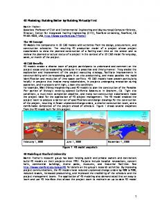
Figure 2.1: Epipolar geometry.  and  are the centers of projection of the images  and   . The plane defined by and its projections  and  is the epipolar plane.  and  are epipolar lines. More recent techniques based on central planar projections use epipolar geometry to interpolate between two or more images of the representation. Given a point of the scene and its projections on two of the representation’s images, epipolar geometry establishes a unique relationship between the two projection points (see figure 2.1). The relationship is given by a 3x3 matrix in homogeneous coordinates, the fundamental matrix, which is independent of the geometry of the cameras used to capture the images. Both projection points and the original point in the scene define a plane called epipolar plane. The epipolar plane passes through the centers of projection of the images, and intersects each image plane at a line called epipolar line. Epipolar geometry was first borrowed from computational geometry by Faugeras and Robert [28]. Its main advantage is that it does not require knowledge of the camera geometries to render new images of the scene. Epipolar geometry has been widely used by Computer Vision researchers to render new perspectives from images captured from the real-world [56] [27] [91] 9

[15]. However, it requires that correspondence between the points be established before new images can be produced. There are many techniques in Computer Vision for establishing correspondence, and most of them have been used by imagebased rendering researchers. The simplest one has a human operator manually selecting corresponding points in related images. More sophisticated techniques rely on segmentation, clustering and classification methods, as well as pattern recognition and other artificial intelligence methods.

2.1.2 Panoramas and Environment Maps Alternative image-based representations use cylindrical instead of planar projections to model scenes. These are better suited for capturing, processing and rerendering panoramas and environment maps. The first two instances of cylindrical representations were QuickTime c VR and plenoptic modeling. QuickTime c VR [16] uses panoramic real-world images to simulate interactive walkthroughs in real-world environments. Like Chen and Williams’ system [17] panoramic images are also stored in a 2D lattice. Therefore, walking is done by hopping to different panoramic views and interpolating between them. QuickTime c VR uses correspondence maps to relate neighboring images in the 2D lattice. Camera panning, tilting and zooming is simulated by using image warping techniques. Finally, QuickTime c VR also allows the representation of objects by capturing multiple images from viewpoints around the object. McMillan’s and Bishop’s plenoptic modeling system [72] uses cylindrical projections acquired at discrete sample locations in 2D space. They also store scalar disparity maps that relate neighboring projections to each other. Rendering is done in three steps. Given a set of viewing parameters, the first step uses digital image

10

warping to remap the closest two 
 samples onto a new target cylindrical projection. The second step then obtains a back-to-front ordering of the image warps using the depth maps of the original projections, and a set of correspondence points between them. Finally, the third step combines the two image warps into a single planar image using filtering and image interpolation to reduce aliasing artifacts. More recent work focuses on creating full-view panoramic images from video streams captured with a hand-held camera. For example, Szeliski and Shum [98] describe a system that is capable of recovering both the camera’s focal length and the relationships between the different camera orientations. With that information, they build a model for full   environment maps that they render using their own hardware rendering algorithm. Alternatively, Wood et al. [104] present a Computer Graphics solution to the problem of generating multiperspective panoramas for cell animation and videogames. Multiperspective panoramas are 2D images containing a backdrop for an animation sequence. The backdrop incorporates a “pre-warped” set of views that typically represents the background of the animation sequence as the camera moves through it. Finally, Sum and He [94] propose an image-based representation for modeling scenes by nesting a set of concentric cylindrical panoramic images.

2.1.3 Image-Based Object Models Most of the image-based techniques described so far focus on models of synthetic or real-world environments for interactive walkthroughs or background environment mapping. Other techniques have been proposed in the literature to build models of single objects or groups of objects. The main difference between both types of models is the orientation of the camera views used to capture the images. Models

11

for panoramas and environment maps use outward looking views, while models for single objects use inward looking views. Outward looking views typically share centers of projection or have them arranged in some sort of lattice. Inward looking views typically share the look-at point usually at the center of the object, while their centers of projection are placed around the object outside of its convex hull. The first example of such a representation is QuickTime c VR’s object movie [16]. An object movie contains a 2D set of images taken from vantage points around a given real-world object. Those images are typically captured using a computer-controlled camera gantry that moves in



increments both horizon-

tally and vertically. Once the images have been captured, they are organized and stored so that the object can be viewed later by rotating it in front of the viewer. Additionally, QuickTime c VR’s object movies allow the representation of animated objects by storing multiple time-dependent images for any given vantage point. In 1996 Max proposed an alternative hierarchical representation to model trees [71]. Max’s representation stores for each element in the tree a set of orthographic projections taken along different directions. Associated to each projection he stores color, alpha, depth and normal information. A different hierarchical representation for single objects was proposed by Dally et al. . They use perspective images captured from vantage points located on the surface of a sphere surrounding the object. Images thus obtained are then hierarchically arranged and compressed to produce a delta tree, a representation that can be efficiently rendered and supports both antialiasing and levels of detail. Yet another object-centered representation was suggested by Pulli et al. [81]. They use inward looking perspective projections to build hybrid models that contain both images and geometry of real-world objects. Given an initial set of images, geometry is recovered and used to build a coarse geometric representation of the tar12

get object. At rendering time the few polygons representing the object are rendered using the image data as texture maps. The problem of Pulli et al.’s representation is that their renderings exhibit polygonal silhouettes. This problem was later addressed by Gu et al. [39] and Sander et al. [85]. Finally, Rademacher and Bishop [82] introduced the concept of multiplecenter-of-projection (MCOP) images. MCOP images are single 2D images that contain information captured from different view points around an object. They are an alternative to QuickTime c VR object movies, since they allow any camera location on a continuous surface, and they store all the image data in a single image instead of multiple images. They are also similar to multiperspective panoramas, but they store inward-looking views instead of outward looking views.

2.1.4 Layered-Depth Images An alternative to storing a coarse geometric model of an object uses depth images or depth maps for hybrid geometry- and image-based representations. Given a color image, a depth map contains a depth value for each of the pixels in the image. The depth value may be an offset value with respect to a plane through the object’s center or a distance to the center of projection of the image. For synthetic images depth data can be obtained from the depth buffer of the graphics engine. For real-world images depth can be computed using one of several Computer Vision methods like depth from motion, depth from stereo, or depth from focus. The first such representation was Max’s as described in the previous section [71]. Later Gortler et al. [37] and Shade et al. [93] introduced the concept of layered-depth image (LDI). An LDI stores color and associated depth information along the rays of a perspective camera. In its simplest form it may contain a

13

single image-and-depth-map pair called a sprite with depth. More complicated representations use multiple pairs of depth-and-color samples arbitrarily placed along each of the camera’s rays. LDIs can be generated using depth data from a hardware graphics engine, a modified ray tracer, or a set of real-world images with an depth computation method like those used in Computer Vision. They can be efficiently rendered on a PC using epipolar geometry for depth sorting and splatting for resampling. An extension to LDI images, the LDI tree was proposed by Chang et al. in 1999 [14]. They use an octree-based spatial decomposition structure to partition space into 3D cells. Then they associate an LDI image to each of the six sides of the octree cells. Chang et al. give algorithms for constructing and rendering LDI trees based on orthographic projections. A different extension of LDIs, the image-based object, was suggested by Oliveira and Bishop [75] to represent single objects. An image-based object consists of six perspective-based LDIs that share their centers of projection with the object’s geometric center. The LDIs are arranged in a cube-like fashion, each of them facing one of the six canonical directions.

2.1.5 Other Related References Other image-based modeling and rendering work was done in image capture and radiance extraction from photographs. Photographs are useful for image-enhanced geometric rendering and for hybrid geometry- and image-based rendering. Debevec et al. pioneered this field by constructing architectural models from a sparse set of views taken with a photographic camera [23]. One year later, Debevec and Malik proposed a method for recovering high dynamic-range radiance from photographs [22]. Debevec and Malik’s method was later used by Debevec to embed synthetic

14

objects into real scenes [20], and by Yu and Malik [106], Yu et al. [105] and Debevec et al. [21] to extract radiance and reflectance information from photographs and generate new images from them with updated illumination effects. Image-based techniques have also been used to extract multi-layer 3D representations from 2D photographs [51] and to design the office of the future [83]. Horry et al. [51] describes a simple method to manually select objects within a single 2D image, then place them at different depths and re-render the resulting 3D model to give a sensation of depth. The office of the future uses wall re-projections of remotely captured images that heavily rely on image-based modeling and rendering techniques. Other related work recently reported includes image-based techniques for soft-shadow rendering [2] and texture mapping with relief [76], a hardware architecture for warping and re-rendering images [80], and an image-based multi-stream video processing system capable of re-rendering new views from virtual cameras in real time [70]. Finally, two surveys of image-based modeling and rendering techniques have been published in the literature by Lengyel [58] and Kang [53], respectively. The reader is advised to consult them for more information and additional references in the field.

2.2 The Plenoptic Function and the Light Field The image-based models described so far attempt to model 3D objects and scenes using 2D images. The images may be parallel or central planar projections, cylindrical projections, spherical projections, LDIs, MCOP images, environment maps or multiperspective panoramas. However, they are still 2D arrays or sets of 2D arrays of pixel data specifically arranged for a given target application. The ques15

tion arises whether a higher-level representation can be found that encompasses all possible image-based representations. The answer to this question is yes. In 1991 two Computer Vision researchers, Adelson and Bergen, defined the plenoptic function to describe everything that is visible from any given point in 3D space [1]. More formally, the plenoptic function gives the radiance, that is, the flow of light, given direction




at any given point


  

in any

for any given time  and any given wavelength  .

For the purpose of our analysis, we consider the plenoptic function to be time-independent, i.e., we only study its representation for static objects and scenes. We also restrict our analysis to a single wavelength. Our results can then be extrapolated to all the wavelengths of our color system, as it is customary in Computer Graphics and Computer Vision. The plenoptic function thus becomes a 5D function


    

of scalar range. Note that this function depends on two geometric

terms, position and direction (see Figure 2.2). Its support is thus the set of all rays in 3D cartesian space. Position is represented by a point direction is represented by a pair

 




in 3D space, while

of azimuth and elevation angles, respec-

tively. An alternative notation for directions represents them as unit vectors



or,

equivalently, as points on a sphere’s surface. The next question that arises is why the plenoptic function. First note that images are 2D “slices” of this 5D function. Hence, the plenoptic function provides a good understanding of how to construct models from images of the real world. Also note that this is irrespective of the shape of the projection surface and the location of the image’s projection center, thus allowing any type of image-base representation. Furthermore, given a set of viewing parameters, we can render the usual perspective projection by evaluating the light field function at the


  

location of the eye

for a discrete set of directions within the field of view. Hence, we can conclude 16

( , )

(x, y, z)

Figure 2.2: Geometric parameterization of the plenoptic function


    

.

that models approximating the plenoptic function are well suited for image-based modeling and rendering.

2.2.1 The Light Field An alternative, but equivalent, representation for image-based modeling and rendering is the light field. The light field was extensively discussed in a classic 1936 book by Gershun, which was later translated to English by Moon and Timoshenko [32]. Gershun was interested in applying field theory, which had been so successful at modeling gravity, electromagnetism and other physical phenomena, to optics and illumination engineering. In Chapter 2 of his book, Gershun defines a set of photometric quantities as part of his theory of the light field. One of them refers to the fundamental concept of brightness at a point in a given direction, a concept, he says, that was first introduced by Max Planck. Gershun argues that this definition is a generalization of the brightness of a light source, which in turn is preferred to the classic definition of brightness as intensity per unit area. Then he characterizes the structure of the light field at a given point by the brightness-distribution solid, a

spatial analogy of the plenoptic function at the point . 17

Unfortunately, his discussion is difficult to follow for the modern computer scientist, since most of the photometric quantities he defines have now been carefully standardized and replaced by radiometric quantities.1 Also, the light-field characterizations he presents in Chapter 5 are based on characterizations of the irradiance, which gives the radiance arriving at a small surface area as a function of direction. Levoy and Hanrahan, who introduced the concept of light field into Computer Graphics [61], point out this problem in Gershun’s analysis. Their original intent was to give an alternative, more appropriate name to the plenoptic function. It turns out that the definition they use refers to Gershun’s brightness as a function of position and direction, the most fundamental quantity in his characterization of the light field. In their paper they actually note the differences between their definition and Gershun’s and refer to a more recent book, The Photic Field by Moon and Spencer [74], for an analysis similar to Gershun’s but based on radiance. Radiance is the radiometric quantity that gives radiant flux per unit solid angle and unit projected area. Like Gershun’s photometric brightness, radiance is a function of position and direction. Formally, a light field represents the radiance flowing through all the points in a scene in all possible directions. For a given wavelength, we can represent a static light field as a 5D scalar function function of location


  


    

that gives radiance as a

in 3D space and the direction

 

the light is trav-

eling. Note that this definition is equivalent to the definition of plenoptic function. However, we prefer the idea of a light field instead of a plenoptic function, mainly 1

Recall that photometry “quantifies” the reaction to light by a human observer, while radiometry quantifies light using physical quantities. An extensive discussion of the differences between photometric and radiometric quantities is beyond the scope of this dissertation. The reader is referred to Chapter 13 of Glassner’s Principles of Digital Image Synthesis [33] for a more detailed presentation.

18

Figure 2.3: Viewing in 2D free space. The eye will never be allowed inside the convex hull of the object. Along the oriented line the value of the light-field function is constant or has the color of the background. because it remains conceptually the same after the changes of representation we describe in the following sections.

2.2.2 4D Light-Field Models The light field made it into the computer graphics literature with the seminal papers on light-field rendering by Levoy and Hanrahan [61] and the Lumigraph by Gortler et al. [36]. Both papers use very similar representations targeted at the representation of objects, but Levoy and Hanrahan’s is slightly more general. The main characteristic of both representations is that they use a simplification of the light-field function that only considers the values it takes in free space. By free space we mean outside the convex hull of an object or inside of a closed environment with static objects. In practice it implies that we only allow inward or outward looking views, as defined above. Given this limitation, the 5D domain of the light-field function can be reduced to 4D, since radiance flows in free space without discontinuities along any given line. To be more precise the support of the light-field function becomes the set of all oriented lines in 3D space, instead of

19

the set of all rays.2 In order to represent the support of the reduced 4D light-field function, both Levoy and Hanrahan and Gortler et al. use the two-plane parameterization (2PP). The 2PP represents each oriented line by its intersection points with two ordered planes, a front plane


 

and a back plane

 

.

Levoy and Hanrahan call such a pair of planes a light slab. They study different orientations for the planes and conclude that it is best to define the planes parallel to each other. For inward looking views they propose separating the planes by a constant distance. For outward looking views they propose placing one plane at infinity. They also describe configurations of multiple light slabs they call slab arrangements. Their goal is to sample the set of 3D oriented lines in way that covers the entire sphere of directions and is as uniform as possible. Alternatively, Gortler et al. only consider models for closed objects. They call their representation Lumigraph and use a set of six slabs arranged as a cube. Each slab contains two parallel planes, as in Levoy and Hanrahan’s implementation. Both papers present acquisition techniques for both synthetic and real-world models. They also describe rendering algorithms for their respective representations and discuss other issues like filtering, interpolation and compression. Their main contribution, however, is the introduction of the 4D light-field paradigm, a new Computer Graphics representation that provides a more formal treatment to image-based modeling and rendering. 2

 




Levoy and Hanrahan [61] place the plane in front of the plane. Gortler et al. [36] use 
 
 the opposite convention, placing the plane in front of the plane [36]. In this dissertation we use the latter convention.

20

2.2.3 Light-Field Improvements For the remainder of this dissertation we restrict our study to 4D light-field models. Hence, we will simply refer to them as light fields. Initially, light fields did not receive much attention in the Computer Graphics literature. The reason is their spatial complexity. Note that a light field is a representation of a 4D function. Therefore, it has very high computational and storage requirements. Most of the light-field work after the original papers thus focuses on efficiency improvements. Sloan et al. propose different methods to trade off lumigraph rendering quality for speed [95]. The simplest speed increase can be achieved by reducing the resolution of either plane discretization at the expense of blurrier images. Sloan et al. concentrate primarily on efficiently managing the resolution of the front plane, the

 

plane. They suggest that a small working set of

 

samples be kept in

memory until a viewer’s position changes and a new set is deemed necessary. A more sophisticated approach applies the same principle to texture memory. Sloan et al. give methods to select image working sets and to rewarp in-memory images instead of loading new images for small changes in the viewing parameters. They also suggest combining some of their techniques with


-blending to implement

progressive transmission and/or progressive rendering. Finally, they describe a lumigraph renderer that runs at a given guaranteed frame rate by using a cost-benefit function to determine which

 

samples to keep in memory at any time.

Alternatively, Regan et al. describe a hardware architecture for interactive light-field rendering [84]. Their architecture is primarily targeted at reducing latency between the user’s input and the image’s updates. Regan et al. use a 2PP representation where the back plane coincides with the computer screen and the front plane is behind the user’s position. To avoid the large storage requirements

21

of a 4D light field they restrict their hardware renderer to 3D light fields that have no vertical parallax. Such a light field is similar to a horizontal-parallax-only hologram as described in Chapter 6. Regan et al.’s system uses a custom mechanical tracker capable of updating the rendering hardware about 100 times per frame. Their rendering system uses uncompressed light fields at a resolution of 128 images of 512x512 pixels each. It is implemented in hardware and is capable of rendering both single images and stereo pairs. The authors use the system to determine acceptable latency values for a set of 12 users. They quantify for the first time the latency requirements on an interactive stereoscopic display. Other light-field work has focused on allowing illumination control of light field data [102] and relating visibility events to the two-plane parameterization [38]. Wong et al. [102] propose a method for recovering BRDF data from multiple images captured according to Levoy and Hanrahan’s representation. For each camera location in the front plane they capture multiple images under different lighting conditions. Lighting conditions are simulated using a directional source that guarantees that light rays hit the target object at the same angle for all back-plane samples. The representation thus obtained is 6D, since each light field sample contains a 2D array of radiance values, one for each directional light source. Alternatively, Wong et al.’s representation can be viewed as a set of BRDF functions located one on each of the back-plane samples. In order to reduce the size of the representation Wong et al. use spherical harmonics to represent the 2D array of radiance values at each

   

sample. They ultimately show that an image-based representation like

theirs overcomes the problem of preventing illumination changes. Gu et al. explore the relationship between the objects in a scene and clusters of similar light-field data of the same scene [38]. In doing so, they consider and

 



slices through the light field. These slices are equivalent to epipolar plane 22

images (EPIs) or images contained in the epipolar planes as defined in Section 2.1.1. Gu et al.’s goal is to provide a theoretical understanding of light-field data based on the geometric information contained in the EPIs. They hope to use that information to devise better rendering and compression algorithms. The work by Halle described later is a good example [44]. Gu et al. also discuss the relationship between the 2PP and Pl¨ucker coordinates and conclude that the 2PP is better for light-field models due to its lower dimensionality. Their work is somewhat related to the work on geometric events and the visibility skeleton by Durand et al. [24] [25]. However, as opposed to Durand et al., they provide a theoretical understanding of light-field data from the geometric events, instead of mathematically describing those events.

2.2.4 Light Fields and Holography Fast rendering algorithms to generate and build 2PP-based light fields have been proposed in the context of computer-generated holography. Recall that 4D light fields and the two-plane parameterization were originally inspired by holography and, specifically, by holographic stereograms [61] [36]. Holographic stereograms are discrete computer-generated holograms that optically store light-field discretizations like those used in Computer Graphics [6] [43]. The relationship between lightfield models and holographic stereograms is described in detail in Chapter 6 of this dissertation. Still, we briefly review here two techniques to efficiently render the images contained in a light field. The first one was proposed by Halle and is called multiple viewpoint rendering (MVR) [44]. Halle’s MVR renders 2PP representations by rendering



slices or, equivalently, EPIs. Halle argues that the EPIs of a 2PP light field are

23

highly coherent. Furthermore, even for complex scenes, they have a simple geometric structure that can be described by small sets of polygon-like primitives. Halle uses this coherence property to generate light-field data by rendering horizontal EPIs using hardware-accelerated polygons. His EPI rendering algorithm takes into account occlusion, specular highlights, texture mapping and environment mapping. His paper also makes a significant contribution to the understanding of geometric events in EPIs. The second approach to rendering light-field models efficiently was proposed Kartch in his dissertation on methods for holographic stereograms [54]. Unlike Halle, Kartch uses a modified 4D Z-buffer algorithm to render all stereogram views in a single pass through each geometric primitive. First, he takes each input triangle and constructs a 4D hyper-polyhedron. Then he performs clipping, pervertex view-independent shading and back-face culling on the hyper-polyhedron in 4D space. After that he subdivides the hyper-polyhedron into 4D simplices (or 4simplices) and applies a 4D scan-conversion algorithm to each of the simplices. 4D scan-conversion is similar to 2D scan-conversion, but it uses four nested loops, one for each dimension. Each nested loops renders a lower dimensional simplex and affects one of the four dimensions of the holographic stereogram. The complexity of Kartch’s algorithm is that of the geometry of the scene, and not the number of radiance samples of the light field representation. Kartch’s work also includes an algorithm for accurately simulating 2D views of the stereogram and compression scheme for stereogram data.

24

2.2.5 Light-Field Compression Other work on light-field compression has been reported by Magnor and Girod [66] [67]. In [66] they describe an MPEG-like scheme that produces better compression rates than those obtained by Levoy and Hanrahan’s vector-quantization scheme [61] [31]. Initially Magnor and Girod transform the input images to YUV color space. Then they average down the chrominance by a factor of two both horizontally and vertically. After that, they DCT-encode a subset of the image, the I-images, as in MPEG coding. Finally, they predict the remaining P-images using four I-images each. The P-images are encoded by breaking them into 16x16 blocks and coding each block using the best of eight different algorithms. The block coding algorithm can thus be chosen depending on the desired transmission rate. According to Magnor and Girod, their method produces compression rates between 80:1 and 1000:1. In [67] Magnor and Girod propose an alternative hierarchical compression method that stores difference images as disparity maps. The method starts by decomposing a light field’s front plane using a quadtree-like structure. Then it arranges and encodes the back-plane images using the tree-like structure induced by the quadtree. The process takes a back-plane image and its four neighbors and computes a disparity map. A disparity map is obtained by decomposing all five images into blocks, then selecting a target block in a neighboring image for each block in the original image. The target block is the best approximation to the original block. It is encoded as a 2-bit index in the disparity map, which in turn is Huffman-coded before transmission. The original image can then be reconstructed by looking up the right blocks of the neighboring images in a target image’s disparity map. The algorithm’s block size is adjustable, allowing compression rates up to 1000:1.

25

2.2.6 Hybrid Models and Surface Light Fields Hybrid models that use the virtues of both image-based models and light-field models have also been suggested. Lischinski and Rappoport [63] propose a model that uses a high-resolution LDI representation for view-independent scene information, and a low-resolution multi-slab light-field representation for view-dependent scene information. The LDI representation stores orthographic projections along the three canonical axes to represent the geometry and diffuse shading information of the scene. To store glossy and specular shading information Lischinski and Rappoport use multiple lower-resolution orthographic LDIs stored as a light-field representation. Rendering starts by warping the diffuse view-independent LDI information, then using the view-dependent light-field data to add reflection and glossy effects. A different type of hybrid model stores both a simple geometric model and a light-field representation similar to the lumigraph. Schirmacher et al. use such a model and propose a method for adaptively constructing and sampling the representation [89]. Their method starts with a simple set of views, then attempts to add a new image from a different view. In order to determine which point of view to use for the new image, several candidates are considered by choosing eye positions between the positions of the original view set. Candidate views are then prioritized using a cost function that takes into account disocclusion artifacts and a radiance error measure. Schirmacher et al. give an adaptive rendering algorithm that produces an initial view-independent rendering using image warping. Then, in a second pass, their algorithm resamples a potentially simplified light-field representation to render the scene’s view-dependent information. An alternative type of light-field representation, the surface light field, was first introduced by Miller et al. [73], then further studied by Wood et al. [103].

26

Their representation is somewhat similar to the representation proposed by Wong et al. [102]. According to Wood et al. a surface light field assigns a color to each ray originating on a surface. Surface light fields are thus good for rendering images of highly specular objects under complex lighting conditions. Their main drawback is that the rendering complexity is no longer proportional to the image size, but also to the geometric complexity of the scene. Miller et al. represent a surface light field using a 4D function parameterized as follows [73]. The first two parameters represent a point within the surface. The last two parameters represent the two orientation angles defining a vector leaving the surface. Miller et al. use a non-linear mapping to map between planar coordinates and the spherical coordinates of the vector. Rendering is done by taking the surface light-field and extracting a color value at each surface point. Color values are extracted using the eye position to determine the coordinates of the corresponding light vector. The algorithm uses cache coherence to speed up rendering. It also allows different DCT-based compression algorithms for the back-plane images. Wood et al. take a more general approach to surface light fields [103]. Specifically, they propose methods for construction, storage, compression, rendering and edition of surface light fields. Their construction methods use both photographs and range image data (like depth maps, as defined above). The light field’s underlying geometry supports levels of detail and small geometric and shading changes. Their work, however, is mostly devoted to the study of better compression schemes for the spherical part of a surface light field. Methods for surface light-fields are related to methods for the acquisition, storage and processing of a surface’s bidirectional reflectance distribution function (BRDF). Debevec et al., for example, use a representation analogous to a surface light-field to acquire and represent the BRDF of a human face [21]. 27

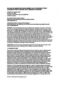
Back Plane

Front Plane Figure 2.4: 2D analogy of the directional and positional biases in the 2PP. The thin lines represent the set of lines generated by joining discrete points on the planes. Note that the lines have seven possible orientations, but the number of lines for each orientation varies between 1 and 4. Also, the distance separating two neighboring lines varies with orientation.

2.3 Uniformity and the Disparity Problem Most of the light-field work published in the Computer Graphics literature is based on the 2PP. This choice of parameterization was primarily inspired by traditional two-step holography [6] [41]. It also simplifies rendering by avoiding the use of cylindrical and spherical projections during the light-field reconstruction process. However, as noted by Levoy and Hanrahan, the 2PP does not provide a uniform sampling of 3D line space, even though that was one of the goals of their representation [61]. Even 2PP models that rely on uniform samplings of the planes are known to introduce biases in the line sampling densities of the light field [10]. Those biases are intrinsic to the parameterization and cannot be eliminated by increasing the number of slabs or changing the planes’ relative positions and orientations [61]. Formally, the statistical and sampling biases of the 2PP are not described in detail until the following chapter. However, we illustrate in Figure 2.4 how the spatial and directional samplings of the lines are affected by the biases of the 2PP. Bi28

ased samplings produce the worst rendering artifacts when the output image spans across multiple light slabs (see Figure 5.1 in Chapter 5 for two examples). The use of separate, individually parameterized slabs makes it difficult to orient filter kernels across abutting slabs. Also, the resulting images exhibit artifacts due to a change of focus in the representation. Even arrangements of 12 light slabs do not suffice to avoid this problem [78]. The problem, named the disparity problem by Levoy [62]. can only be solved by choosing a different parameterization. In this section we study some of the alternative parameterizations proposed for the light-field function. Two of them provide an isotropic representation for the directional support that entirely avoids the disparity problem. In Chapter 6 we also show how a modern one-step holographic stereogram production system can benefit from isotropic parameterizations.

2.3.1 Alternative Parameterizations Three alternative parameterizations have been proposed for light-field representations. Two of them are based on spherical, or isotropic, parameterizations that are intended to reduce or remove the biases of the 2PP, providing renderings of equal quality from all points of view [10] [11]. The third, more recent one is a modified 2PP where the positional and directional dependencies of the light-field have been decoupled, thus reducing the number of biases in the representation [52] [13]. The first two parameterizations rely on the concept of uniform light field, a concept that was studied independently by Lerios, and Camahort and Fussell. In a uniform light field, a uniform random sampling of line parameters induces a uniform sampling of lines. Light-field models satisfying this property are statistically

29

invariant under rotations and translations. The concept was introduced in a joint paper by Camahort, Lerios and Fussell [11], that proposed two uniform parameterizations: the two-sphere parameterization (2SP) and the sphere-plane parameterization (SPP). The 2SP, proposed by Lerios, represents a line by its intersection points with a sphere. The SPP, proposed by us, gives the direction of the line, then places it in 3D space using its intersection point with a plane orthogonal to it. After the publication of [11] we changed the name of the 2SP to direction-and-point parameterization (DPP). The DPP is one of the main contributions of this dissertation. Together with the 2PP and the 2SP, we describe it in detail in the following chapters. The third parameterization was introduced by Isaksen et al. [52] and Chai et al. [13]. Isaksen et al. parameterize a line by its intersection with two surfaces, a camera surface and a focal surface. The 2PP can thus be seen as a specialization of their representation. However, unlike the 2PP, each of their cameras contains a separate image plane, which is also part of their representation. Chai et al. use a similar camera arrangement, but they assume that the camera surface is a plane. In this dissertation we study the more general representation of Isaksen et al. However, we assume that all the cameras have the same intrinsic parameters, that is, the same image size, image resolution and focal length. Each line is then parameterized by its intersection points with the camera surface and the closest camera’s focal surface. These, like the 2PP and the 2SP, are all instances of the two-points-on-two-surfaces parameterization, where an oriented line is represented by its intersections with two surfaces. In this case, however, we can remove the dependency of the representation on a specific camera by representing the second intersection by a direction. We call such parameterizations point-and-direction parameterizations (PDPs). The main goal of Isaksen et al. and Chai et al. is not uniformity. Instead, 30

they study the amount of geometrical and textural information necessary to properly reconstruct the continuous light field. Isaksen et al. analyze their representation in both ray-space and the frequency domain [52]. They also show how their representation can be used to obtain effects such as variable aperture and focus. Finally, they provide an application of light fields to the production of an autostereoscopic display based on integral photography. Chai et al. take a different approach based on the spectral sampling theorem [13]. They use Fourier analysis to establish a relationship between the scene’s geometric complexity, the number of light-field images, and the resolution of the output image. They give minimum sampling rates for light field rendering, and a minimum sampling curve in joint image and geometry space. Using their analysis, they show how to associate different depths to the light-field samples to provide better image reconstruction.

2.3.2 Advantages of Uniformity We just made a strong case for uniform light-field representations. We argued that uniformity guarantees light field invariance under rotations and translations, thus allowing the user to move freely around a model without noticing any resolution changes. These are not the only advantages of a uniform representation. The ability to sample the light field by taking uniform samples of the parameters of its support has other advantages. A uniform sampling guarantees constant error bounds in all dimensions of the light field, so provisions can be made to reduce or avoid doing interpolation at all. When sampling a function whose variation is unknown a priori, uniform sampling provides a good preview of the function, that can later be refined as more information about the function is known. Also, compression theory often makes the assumption of uniformly spaced samples. For instance, the discrete

31

Fourier transform assumes that its input is a sequence of regularly spaced function samples. Uniform models can nonetheless be undesirable. For certain models we may prefer specific directional and spatial biases. In this dissertation we show that DPP representations support adaptivity in both the directional domain and the positional domain. In the directional domain, we use a subdivision process to construct a hierarchical sampling of directional space that can be locally refined depending on the characteristics of the model. In the positional domain we store images that can benefit from well-known adaptive structures, like quadtrees and k-d trees. Adaptivity can be steered using either geometric measures, radiometric measures or both. This can be useful for highly asymmetric objects, view-dependent representations like fly-by’s, and foveal vision.

2.4 Discussion A primary goal of image-based modeling and rendering is to replace geometric models by more efficient image-based models. General geometric models are viewindependent; they are invariant under rotations, translations and perspective projections. Note that this property is stronger than the uniformity property of Camahort et al. [11]. In fact, in [11] they ignore certain geometric corrections required by the image registration process as characterized by the fundamental law of illumination. The problem is a more general one. Current art fails to formally analyze how a light-field parameterization affects the rendering process. Even though uniform light-fields were introduced to guarantee invariance under rotations and translations, their mathematical foundations were never presented and there are still important open issues relating unifor32

mity to perspective corrections and the rendering process. For example, there are correction factors associated to the geometry of projections that have been ignored in both the continuous and the discrete domains. Furthermore, nobody has carefully studied the relationship between the different representations and the artifacts introduced by their discretization. In this dissertation, we examine the sampling biases introduced by both planar and isotropic light-field models. This is done first by examining the properties of the various parameterizations in continuous line space. We identify the sampling biases introduced by these parameterizations and derive the corrections needed to provide view-independent sampling. We examine existing implementations in terms of their success in eliminating sampling biases and providing view independence. We provide a discrete error analysis of these models in order to determine error bounds for them. This analysis solves three important open problems: (i) how to position the planes of the two-plane and direction-and-point parameterizations, (ii) how to place the discretization windows within those planes, and (iii) how to choose the resolutions of each window. Finally, we quantify the aliasing artifacts introduced by each implementation. Given the motivations of the various models, we might expect that models based on planar parameterizations are superior for directionally-constrained applications and that isotropic models are superior for view-independent applications. However, our results show that isotropic models are superior in both cases. The reason is that the nonuniform sampling resulting from planar parameterizations causes greater sampling variations over an individual projection window, resulting in over- or undersampling in some portions of the window. We conclude that an isotropic model based on a direction and point parameterization has the best view-independence properties and error bounds for both types of applications. 33

We demonstrate the view-independent rendering quality obtainable from the direction-and-point model. The absence of large-scale artifacts over a wide range of viewing positions is not obtainable with planar parameterizations. We then demonstrate the advantages of this model for the generation of holographic stereograms. In spite of the fact that planar parameterizations were inspired by traditional two-step holography, we use a more modern one-step holographic process to demonstrate that the direction-and-point parameterization produces image quality indistinguishable from that produced by a two-plane method. Furthermore, in our example hologram the planar parameterization uses nearly twice the number of light-field samples for a typical field of view of 

. Since the production of modern, large-

format holograms can entail the manipulation of terabytes of data, this can be a significant advantage indeed, especially as better hardware is built to provide even wider field of views.

2.5 Outline of this Dissertation Our presentation starts with an analysis of continuous light-field parameterizations and their geometric relationship to perspective projections. We characterize the correction factors required by each parameterization and compare them in terms of ease of implementation. In Chapter 4 we survey current discrete light-field implementations and their rendering algorithms. We describe our implementation of a DPP-based light-field modeling and rendering system in detail. We describe our representation and give construction and rendering algorithms. We In Chapter 5 we discuss rendering artifacts affecting current light-field models. To characterize those errors we define two geometric error measures related to the support of the light-field function: a directional measure and a positional 34

measure. We use those measures to construct optimal models of a canonical object using the current light-field implementations. We also define a measure that quantifies aliasing artifacts for all representations. We compare all three implementations in terms of geometric error bounds and the aliasing measure. In Chapter 6 we illustrate the application of 4D light fields to holography. We present a system that produces holographic stereograms based on both planar and isotropic light-field models. We compare both representations and their suitability for holographic-stereogram production. We conclude this dissertation with a discussion and directions for future work.

35

Chapter 3 Continuous Light-Field Representations We are concerned with the representation of the support of the 4D light-field function. The support is the set of oriented lines in 3D cartesian space, a 4D space. 1 We want a line parameterization such that uniform samplings of the parameters result in a uniform sampling of lines. We thus study different parameterizations of the set of oriented lines in the continuous domain. Then we relate continuous parameterizations to statistical uniformity and sampling uniformity.

3.1 4D Light-Field Parameterizations We describe the four parameterizations that have been proposed in the literature. 1

It is easy to visualize how the set of oriented lines is a 4D space by noting that any oriented line can be uniquely represented by its direction and its intersection point with the unique plane orthogonal to its direction that contains the world’s origin. A direction can be represented by two angles, giving azimuth and elevation with respect to the world’s coordinate system. The intersection point with the plane can be represented by its two cartesian coordinates with respect to a coordinate system imposed on the plane.

36

The Two-Plane Parameterization (2PP) It was introduced by Levoy and Hanrahan [61] and Gortler et al. [36]. 2PP is a short form for two-points-on-two-planes parameterization. The 2PP represents a line by its intersection points with two planes. Levoy and Hanrahan studied different orientations for the planes and concluded that it was best to define the planes parallel to each other. Gortler et al. use the same convention. Both implementations use multiple pairs of planes to cover the entire sphere of directions. In this Chapter, however, a single pair of planes suffices to carry our analysis. The Two-Sphere Parameterization (2SP) It was introduced into Computer Graphics by Sbert, who applied it to the solution of the radiosity problem [87]. Lerios adopted it for his spherical light field representation which was reported in [10] and [11]. Like the 2PP, 2SP is a short form for two-points-on-two-spheres parameterization. It parameterizes a line by its intersection points with two spheres. Typically, both spheres are the same, tightly fit around an object like a bounding ball. The Point-And-Direction Parameterization (PDP) The PDP was never introduced as such. Instead we classify the parameterizations of Isaksen et al. [52] and Chai et al. [13] as PDP parameterizations. They are modified 2PPs that decouple the directional and positional dependencies of the light-field by defining a different window for each point in the camera plane. Although the windows are different, they are translated copies of the same window. If we choose the window to be spherical instead of planar, we can represent each line by its intersection with the camera plane and a direction given by the intersection point on the spherical window. The Direction-and-Point Parameterization (DPP) The DPP is one of the main contributions of this dissertation. It was previously reported in [10], [11] and [9]. It parameterizes an oriented line by its direction and its intersection with a plane 37

orthogonal to its direction. The plane is typically the unique plane that contains the origin and is orthogonal to the line. The DPP is not new to Computer Graphics. It was previously used in areas like ray-classification [4], global illumination [8], characterization of visibility events [24], rendering of trees [71], and progressive refinement for ray tracing [40]. Our DPP models mostly resemble Max’s [71], but he uses a fixed set of 22 directions and stores some additional non-radiometric information for each sample.

3.2 Parameterizations and Uniformity We know that uniform light-field representations are desirable because they are invariant under rotations and translations, they solve the disparity problem, and they guarantee constant geometric error bounds in the parameters of the light field [11] [9]. However, we have not formally defined light-field uniformity, neither have we shown how uniform light fields satisfy those properties. We begin with the definition of light-field uniformity proposed in Camahort et el.’s paper [11]. We define light-field uniformity as statistical uniformity in the continuous domain and sampling uniformity in the discrete domain. We apply both concepts to the support of the 4D light field.

3.2.1 Statistical Uniformity A continuous light-field parameterization is statistically uniform when the following condition is met. Statistical Uniformity. For any set of uniformly distributed light-field parameters, the set of oriented lines represented by those parameters is 38

uniformly distributed over the space of all oriented lines. We call a set of oriented lines a pencil of lines. In order to study the statistical uniformity of a pencil of lines we associate to it a measure that quantifies the “amount” of lines contained in it. From a purely statistical point of view it would be more appropriate to define a density function on the set of oriented lines. However, the entire set of oriented lines is too broad a domain for a computer implementation of the light-field function. We are interested in modeling 3D objects and scenes for discretization and implementation on a computer. Such models are typically bounded, and so are the sets of lines that intersect them. Therefore, we are only concerned with the representation of bounded sets of oriented lines intersecting a given target object or scene. Given a line measure function and the total finite measure of the lines intersecting the target object, we can easily define density values for any pencil of lines within the given line set by dividing its measure by the total measure of lines of the model. In this dissertation we assume that our 3D models are bounded. The set of lines intersecting the model is also bounded, and so is the domain of the light-field function. Under these assumptions we study the statistical uniformity of a pencil of lines by looking at its measure of lines. Measures of lines have been studied in Integral Geometry and Geometric Probability [86] [97]. For example, the measure of lines through two surface patches has been shown to be related to the form-factor kernel, as pointed out by Sbert [87] and Levoy and Hanrahan [61]. This case is relevant to 2PP and 2SP light fields, where a line is parameterized by two points  and  on two surfaces (see 
 Figure 3.1). The measure of lines passing through the two differential areas 

39

dA2

2 r

1

dA1

P 2

P 1   and Figure 3.1: The measure of lines passing through two differential areas  . The dashed lines represent a polyhedron bounding the pencil of lines defined  and   . by and





around  and  is given by the form-factor formula










 












 

(3.1)

This measure depends on the angles between the normals to the surfaces and the line connecting them. It also depends on the distance between the two areas. If we

 to be uniformly distributed over each surface patch,  and   are constant, but the measure 
varies with  the positions and relative orientations of  and   . choose the points



and  then the area measures

Common examples of two-point parameterizations are those based on (i) two parallel planes, like the 2PP, (ii) a sphere, like the 2SP, and (iii) two arbitrary surfaces, like the parameterization proposed by Isaksen et al. [52]. For the 2PP Equation 3.1 becomes

where









 





is the angle between the line joining

planes, and



 



and



and the normal to the

is the distance between the two planes (see Figure 3.2). Note that the

measure of lines depends on five constants, 40

,

, 

, 

and 

, and a variable

dt

P 1

du

β

d

ds

β P2

dv

Figure 3.2: The measure of lines passing through two differential areas given by the parameter measures ,  ,  and  and located on two parallel planes separated units. term 



related to the relative orientation of the pencil and the planes. This is the

source of the directional biases of the 2PP. As the pencil forms an increased angle

 . Conversely, with the plane’s normal, the measure of lines decreases with   

the measure of lines reaches its maximum when the pencil intersects the plane at a right angle.

3.2.2 Sampling Uniformity The directional biases of the 2PP can be corrected for, by choosing non-constant values of

, 

, 

and 

. Depending on the orientation of a given pencil, we

choose the differential areas such that the measure of the pencil is the same for all pencils. In practice, that requires discretizing the light field using non-uniform samplings of the parameter spaces. This brings us to the concept of sampling uniformity. A discrete light-field representation is uniformly sampled when it satisfies the following condition.

41

Sampling Uniformity. A uniform sampling of the parameters of the light field induces a uniform sampling of the set of oriented lines in the light-field support. The relationship between statistical and sampling uniformity is critical to understand why the biases of the 2PP are so difficult to eliminate. We can state that relationship as follows. Relationship Between Statistical and Sampling Uniformity. Given a continuous light-field parameterization that satisfies the condition of statistical uniformity, we can obtain a discrete light-field representation that satisfies the condition of sampling uniformity by uniformly sampling each of the continuous parameters separately. However, if the continuous light-field parameterization is not statistically uniform, a uniform sampling of its parameters will not induce a uniform sampling of the support of the light field. This is the case of the 2PP, that requires the parameters of the support to be corrected for biases during discretization and sampling. Such non-uniform samplings are difficult and costly to implement, and may render a representation impractical. An alternative solution chooses a light-field parameterization that satisfies the property of statistical uniformity. Given such a parameterization, we use the above relationship to obtain a uniform sampling as follows. We develop a deterministic scheme that generates sets of parameter values regularly distributed throughout their domains. And we take samples of the light field using these sets of parameter. The uniformity properties guarantee that the samples will be uniformly spaced in the domain of the light field. 42

This uniform sampling process has a very important advantage: it entirely avoids the definition of a distance measure between two oriented lines. Such measures have been previously proposed in the Computational Geometry literature [3]. They typically separate the positional and directional dependencies of the light-field function, and choose an euclidean distance and an angular distance for each parameter set, respectively. Still, the choice of an euclidean distance highly depends on the application, and there is no clear understanding on how to combine both distance measures into a single one. The problems with distance measures are better avoided altogether.

3.2.3 Uniform Parameterizations We concluded that a continuous light-field parameterization has to be statistically uniform to facilitate the construction of uniformly sampled light-field models. Statistically uniform parameterizations have been studied in Integral Geometry [86] [97] and Computational Geometry [77]. They have been applied to ray casting [77] and form-factor computation [87]. At least two parameterizations are known to support the selection of pencils of lines following a uniform distribution, the 2SP [87] and the DPP [11]. To simplify the following discussion we use statistical and sampling terminology interchangeably. The random processes that allow the selection of uniformly sampled lines for the 2SP and the DPP are illustrated in Figure 3.3. We assume that the target object is placed inside of a bounding sphere. The bounding sphere fits tightly around the object, and is typically scaled to unit radius and centered at the origin. We model the object using a light-field representation that stores a radiance sample for each oriented line that intersects the bounding sphere. The choice of line representation

43

C L

L

Q P

P

Figure 3.3: Two ways of uniformly selecting a random oriented line intersecting a 3D sphere. Left, select two random points and uniformly distributed over the sphere’s surface and join them with a line . Right, select a random great circle  with uniform probability over all great circles and a random point uniformly distributed over  ’s surface, and choose the line orthogonal to  through . depends on the parameterization. For the 2SP we use a process such that choosing two points on the sphere with uniform probability implies that the line joining the points follows a uniform distribution over the set of all lines intersecting the sphere. For the DPP we use a process such that choosing an oriented great circle and a point on its plane both following uniform distributions implies that the line orthogonal to the great circle through the point follows a uniform distribution over the set of all lines intersecting the sphere. Note that choosing an oriented great circle is equivalent to choosing its normal, which is the same as choosing a point on the unit sphere. The statistical uniformity of the 2SP can be proved using the form-factor formula, Equation 3.1, and the geometry of the sphere. The measure of lines through  the two differential areas  and   on the sphere’s surface is given by  














 









 

 






44




 










 





R cos

R cos

dA1

dA2

R C

Figure 3.4: 2D analogy of the 2SP and its form-factor geometry. In the 3D sphere 

and the distance  between   and   is equal to     .  is the constant radius of the sphere.














where














 

is the (constant) radius of the sphere (see Figure 3.4). This result was

first incorporated into form-factor computations by Sbert [87]. It shows that the measure of lines through two differential areas on the sphere is proportional to the product of the measure of points in each area. Hence, if the differential areas are uniformly distributed over the sphere’s surface, then the pencil of lines follows a uniform distribution.2 The statistical uniformity of the DPP follows immediately from the parameterization. A differential pencil of lines is given by a differential area of measure  around the point , and a differential solid angle around the normal to the   great circle  containing (see Figure 3.3 right). Since the differential area 2

Surprisingly, this property is only satisfied by 3D balls and pencils of 3D lines in 3D space. The reader is advised to try to determine the measure of lines of a similar 2D representation on the circle. A general formula for balls and convex objects of any dimension can be found in Santal´o’s treatise on Integral Geometry [86].

45

is orthogonal to the differential solid angle



, no corrections are necessary and the

measure of lines is simply the product of both measures









Note that this formula is similar to the measure of a 2SP pencil, since setting  
  produces an equivalent result.






3.2.4 Discussion Uniform parameterizations were introduced to support continuous light-field representations that are invariant under rotations and translations. They allow the construction of discrete light-field models based on sampling processes that avoid the need of a distance measure in oriented line space. They guarantee constant error bounds for all the samples of the discretization, thus preventing both over- and undersampling and gross discretization errors. If we compare them to standard geometric models, uniform light fields appear to be a competitive alternative. Unfortunately, they ignore an important property of geometric models, view independence. View independence guarantees that a model is invariant under rotations, translations and perspective projections. Since this feature is usually expected of a general geometric model, it should also be expected of a general radiometric model. We study a light field’s view independence by analyzing the process of rendering from a light-field representation.

3.3 Rendering from Continuous Light Fields We want to accurately model the process of registering images from a light-field representation. Such a goal imposes additional conditions on the line parameteri46

d

d dA S

dA P

r

r

Figure 3.5: Geometry of the fundamental law of illumination. Left, the irradiance 
arrives at the registration surface through a spherical differential area . Right, the irradiance arrives at the registration surface through a planar differential area   . In both cases the pencil of lines 
represents the support of the irradiance function. zation. Consider the process of image synthesis. An ideal light-field representation would avoid introducing additional biases at rendering time. Such a representation would take a uniformly distributed random pencil of lines in the light field’s parameter space and project it onto the projection surface, so that the projected area also follows a uniform distribution over the surface. Under such assumption, arbitrary views of the model would be generated without sudden resolution changes or representation-dependent artifacts. Additionally, it would ensure that discretization errors in parameter space produce minimal errors at rendering time, and not just in the representation. In order to obtain such a parameterization we look at the process of image registration (see Figure 3.5 left). It is characterized by the fundamental law of

47

illumination [32], that gives the irradiance at the registration surface as a function of incoming radiance

Here





 










is the angle between the normal at the registration surface and the incoming


light direction, and  is the distance to the light emitter. This law introduces two new biases associated to the registration process: the Lambertian attenuation term  


 and the inverse-square law  . Note that these are geometric terms related

to the support of the radiance function 















is the measure of lines arriving at the registration surface and is a 
differential area obtained by intersecting with a hemisphere of radius  located where




in front of the surface (see Figure 3.5 left). Images are usually obtained using central planar projections. More sophisticated models for cameras and the human eye have been proposed, some of them with spherical projection surfaces [55] [33]. Still, rendering in computer graphics is mostly done using the pinhole camera model and perspective projections. If we consider the projection plane to be orthogonal to the normal at the registration surface and located at a distance  , the irradiance becomes





  








We use this formula to establish a geometric relationship between




and the differ-

ential area it intersects on the projection plane (see Figure 3.5 right):





  






 

Ideally we want a parameterization such that for any perspective projection 
 and any uniformly random pencil of lines of measure , the measure of the 48

intersection area of the pencil with the projection surface depends linearly on the product of the measures of the line parameters. A representation based on this ideal parameterization would be view-independent, that is, statistically invariant under rotations, translations and perspective projections. Images obtained from it would not be biased towards certain viewing positions and/or directions, and we would not need to correct for potential biases at rendering time. Using the sampling process described above, we could discretize the light field by uniformly sampling each of the parameters of the support and constructing a uniform sampling of oriented line space. At rendering time, uniform pencil samples would project onto the projection plane onto discrete area samples of the same area. Since all area samples would be of the same area, discretization errors would have the same upper bounds for all samples. Error bounds would be minimized. and we would have the best possible discrete light-field representation. We will see that such an ideal representation is unlikely for 4D light fields. Instead, we introduce an alternative representation that is only biased towards a specific viewing distance. In practice, such a bias can be easily corrected for by using a distance-dependent discrete multiresolution representation.

3.3.1 Two-Point Parameterizations We start our view-independence analysis with two-point based parameterizations. Figures 3.6 and 3.7 show the geometric correction factors involved in rendering a 2PP-based and a 2SP-based light-field representation, respectively. In both cases 
arriving at the center of projection  through a we give the measure of lines   differential area as a function of the parameters of each representation. For the

49

du dv D

ds dt

dA S dA P C

r d

S

(u,v) plane

(s,t) plane

P

Figure 3.6: 2D analogy of the geometry involved in rendering a 2PP-based lightfield representation.  is the center of projection. is a spherical projection sur   face. is a differential area on . is the projection plane. is a differential area on .
is the distance between  and the front plane of the parameterization. 


is the angle at which the differential pencil of measure intersects that plane. is the (constant) orthogonal distance between the two planes. 2PP the measure of lines is  

















 

 









 














 







as shown in Figure 3.6. For the 2SP the measure is 



Solving for



















  











gives the area measure on



  















and for the 2SP







 

 

 








 






 




 


50

 









 





  

 

as a function of the parameters of

each representation. For the 2PP it is








  



 

 

   




 

 






 

dA 2 D dA 1 R

dA S C

R dA P

r

S P Figure 3.7: 2D analogy of the geometry involved in rendering a 2SP-based rep resentation. All the variables have the same meaning as in Figure 3.6. is the (constant) radius of the sphere. To render an image from either light-field representation we have to correct for two types of biases, positional biases and directional biases. The correction factors depend on three sets of two variables each: 

and , which are constant camera parameters, invariant for a given camera


and independent of the light-field representation,  and , which are constants of the light-field representations, characteristic of each representation and independent of the viewing parameters; and




and , which represent the relative positional and directional dependencies

of the camera and the light-field representations. 

, ,



and


introduce positional biases, and




and



introduce directional biases.

 The first correction factor is the distance-squared factor 




 , that stems

from the inverse-square law. It can be can be taken into account in either of two ways: (i) by using a multiresolution representation, for example, a set of 51

mipmapped images, or (ii) by extending the light-field representation to handle the 5th dimension of the support. The second factor, the directional term    


, depends on the camera

geometry and can only be corrected for at rendering time. If the projection surface were a sphere it would be equal to one. In practice, the effect of this bias is only relevant at points near the boundaries of the rendering window. The effect has been studied in optics where it is relevant to lens design and it is known as vignetting. In Computer Graphics, however, it is normally ignored, even in the highly camera models [55].

The  term depends on the orientation of the light-field model with re-

spect to the camera, and it can be corrected for by using a look-up table or by

storing different samples sets for different values of . Either approach requires extra storage and can be very expensive depending on the dataset. The main problem, however, is that both representations require different distance-squared corrections for the first and second surfaces. The problem is aggravated by the fact that the correction factors for the second surface depend on both




and , which in turn depend on the relative position and orientation of the

camera and the representation. To correct for these factors we need different samplings for the first and second surfaces. Additionally, we need to store separate

samplings for all the possible values of . Even if we decided to give up statistical uniformity, building a discrete light field with the necessary sampling corrections would be highly impractical. The problem is that two-point parameterizations tie together the directional and positional dependencies of the light field.

52

D

du dv

d

dA S dA P C

r

P

S

Figure 3.8: 2D analogy of the geometry involved in rendering a PDP-based representation. All the variables have the same meaning as in Figure 3.6. is a differential solid angle.

3.3.2 Point-and-Direction Parameterizations A first solution to this limitation decouples the positional and directional dependencies of the light field. A PDP-based light-field representation replaces the second point point of a two-point parameterization by a direction. That way it avoids the biases and correction factors related to the second point. Figure 3.8 shows the geometry involved in rendering a PDP-based light field, when the point varies over a 
  planar surface. The measure of lines through is 



We now solve for





















  









and obtain













 














 

  













The correction factors are the same for the point as for the first point in two-point parameterizations. For the direction, however, we only have correction factors related 53

D

du dv

dA S dA P C

r

P

S

Figure 3.9: 2D analogy of the geometry involved in rendering a DPP-based representation. All the variables have the same meaning as in Figure 3.6. to the viewing parameters. Hence, the PDP solves some of the problems associated

with the  bias of two-point parameterizations. Can we remove the same bias

from the first set of parameters and  ?

3.3.3 Direction-and-Point Parameterizations Suppose that we switch the order of the light-field parameters. First, we determine the direction of the 4D line. Then we place it in 3D space by intersecting it with a plane orthogonal to its direction. DPP-based models expect the light-field data to be stored and accessed in that order. Otherwise, they sample oriented line space like the other models. The surface for the point can be any surface, but a planar surface orthogonal to the line’s direction introduces the fewest correction factors. 
Those correction factors are shown in Figure 3.9. can be expressed as





 



















 


54










Again we solve for





and obtain






 

 






 







 






The    term no longer affects the parameters of the light field. Only the pro-

jection biases and the distance-squared term




need to be considered in the rep-

resentation. The directional projection bias  




accounts for vignetting and

is usually ignored in Computer Graphics. For the combined distance-squared term 




we may store a prefiltered multiresolution representation or sample along

the fifth dimension of the light field. Adopting the second solution implies modeling the 5D light field. Note that the fifth dimension of the light field represents changes along the oriented lines of the 4D light field. If we store samples taken along the oriented lines, then we are effectively storing a discrete representation of the 5D light field. Such representations are beyond the scope of this dissertation, but we can conclude from the above analysis that DPP-based models can be easily extended to represent the 5D light field. Whether DPP-based models are better than ray-based models or other representations for 5D light fields remains to be shown.

3.4 Discussion We have studied continuous light-field representations based on four different parameterizations of 4D oriented line space. An important issue is invariance of a representation under rotations and translations. Our study relates these invariance properties to the concepts of statistical uniformity and sampling uniformity of a representation. Statistical uniformity applies to continuous light fields and is a prerequisite for sampling uniformity and the construction of uniform light-field dis55

cretizations. We study the uniformity of the four parameterizations and conclude that only two satisfy the statistical uniformity property as defined in Section 3.2. We argue that the notion of uniformity, as introduced by Camahort et al. [11], is too weak. We impose the additional condition that a light-field parameterization be invariant under perspective projections. We call this property viewindependence. Our goal is to guarantee uniformity not just in the representation, but also during and after the rendering process. We analyze the biases introduced by the four parameterizations at rendering time. We determine the correction factors needed by each parameterization to guarantee view-independence, and we outline possible ways to implement those correction factors. We conclude that none of the current light-field parameterizations is viewindependent. Even though we have not proved it, it is unlikely that such a parameterization exists. We show that among the current parameterizations the DPP introduces the least number of biases at rendering time. We also show that DPP models augmented with a multiresolution image representation require only projectionrelated corrections at rendering time. The images in Figure 4.14 illustrate the view independence feature a DPP model. The images in Figure 4.15 illustrate how the directional and positional resolutions of a DPP model can be separately controlled, an additional property of DPP models, and how spatial multiresolution can be implemented using available texture-mapping hardware.

56

Chapter 4 Light-Field Implementations Implementing a light-field model for Computer Graphics rendering is similar to implementing a computer model of any other function. It starts with a process that generates or captures a set of discrete samples to build the model. Samples are then organized and stored so that they can be efficiently retrieved for rendering. At rendering time the light-field function is reconstructed from the samples to produce an approximated continuous light field. That light field is then resampled for display on a discrete computer screen. These steps are illustrated in Figure 4.1. Interpolation is typically used during the reconstruction of the light-field function. Filtering may also used during light-field sampling and resampling to help reduce or eliminate aliasing artifacts in the rendered images. A light-field implementation can be characterized by its representation, its storage scheme, and its construction and rendering algorithms. In this Chapter we review these characteristics for three of the current light-field implementations. We also describe our DPP-based light-field implementation in detail. Our description includes other implementation features like interpolation, multiresolution, compression, LOD interpolation, and adaptive frame-rate control. 57

ACQUISITION LIGHT FIELD FUNCTION

FILTERING

FILTERED FUNCTION

SAMPLING

DISCRETE REPRESENTATION

RENDERING DISCRETE REPRESENTATION

RECONSTRUCTION

APPROXIMATED FUNCTION

RESAMPLING

DISCRETE IMAGE

Figure 4.1: The different steps required in a discrete 4D light-field implementation.

4.1 Discrete Light-Field Models Six light-field implementations have been proposed in the literature [36] [61] [11] [52] [13]. In this Section we survey three of them: the two 2PP-based implementations of Gortler et al. [36] and Levoy and Hanrahan [61], and the 2SP-based implementation presented in Camahort et al. [11]. All of them have been shown to support a similar set of basic features. We describe how they acquire, discretize and stored the light field function. We also relate their storage schemes to each implementation’s rendering algorithm. We classify the storage schemes into samplebased and image-based schemes and describe rendering algorithms for each storage scheme.

4.1.1 2PP-Based Implementations 2PP-based light-field implementations have been proposed by Levoy and Hanrahan [61] and Gortler et al. [36]. Both implementations discretize the light-field support by imposing rectilinear grids on each of the two planes of a light slab. The sampling rates for the horizontal and vertical dimensions are usually the same, but the rates

58

for the front plane may be lower than the rates for the back plane. The papers do not discuss the position and size of the discretization windows within each plane. Neither do they address the problem of how to place the planes with respect to the target object. In the following Chapter we show how plane positions and window positions, sizes and resolutions can be optimally chosen for 2PP-based models. We also show that those choices are key to determining and minimizing the geometric errors incurred by the representation. For now, however, we assume that the choices of windows and plane positions allow sampling all the lines intersecting the target object in some way. Isaksen et al. [52] and Chai et al. [13] study the positioning of the planes for their modified 2PP representations. Chai et al. also address the issue of using more than one back plane with an associated depth each for more accurate resampling. However, their parameterizations are different from the original 2PP, and their analysis only applies partially to 2PP-based models. A different problem of 2PP-based models as that a single slab only covers a limited amount of directions, typically one sixth of the sphere. The solution to this problem uses multi-slab arrangements that guarantee that all the lines through the target object are being sampled. Levoy and Hanrahan propose different types of arrangements depending on the application and the target scene [61]. For the lumigraph, Gortler et al. implement six pairs of planes arranged in a cube placed around the target object [36]. Neither of Isaksen et al. and Chai et al. address this problem in their papers. Features common in early 2PP-based implementations are acquisition from real-world objects, filtering during sampling, and interpolation during light-field reconstruction. Levoy and Hanrahan implement 4D filtering by using both 2D pixel 59

filtering and 2D aperture filtering when building a model from synthetic images. Gortler et al. introduce an interesting method, called push-pull, to construct a filtered lumigraph representation from a sparse set of arbitrary images captured with a digital camera. At rendering time, Levoy and Hanrahan use quadralinear interpolation, while Gortler et al. use linear-bilinear interpolation, an approximation to quadralinear interpolation that uses graphics hardware and -blending for improved


rendering speed. An important feature unique to the lumigraph is the inclusion in the model of a coarse geometric representation of the target object. The geometry is used to perform depth correction on the light-field data. Depth correction allows a light-field sample to be placed at the point along its support line where the original geometry was intersected. The light-field renderer can use that information to depth-sort the samples and provide a better reconstruction algorithm. Depth correction is described in detail later in this Chapter, as part of our DPP-based implementation. Finally, Levoy and Hanrahan propose a light-field compression method based on vector quantization [31] that allows storing an entire model in memory and supports decompression and rendering at interactive rates.

4.2 A 2SP-Based Representation The 2SP represents each line passing through an object by its two intersection points with a sphere tightly fit around the object [10] [11]. Discretizations of the 2SP are based on nearly-uniform tessellations of the sphere that satisfy certain hierarchical multiresolution properties. Such tessellations subdivide the sphere’s surface into (nearly) equilateral, (nearly) identical spherical triangles (see Section 4.3 for a more detailed discussion). For each ordered pair of spherical triangles the 2SP-based 60

representation stores a light-field sample taken along the line passing through the triangles’ centers. The simplest way to store the 2SP is a two-dimensional array, mapping each ordered triangle pair to a light-field sample. At rendering time rays from the eye through the image pixels are intersected with the sphere of the representation. Given the indices of the triangles where the intersections occur, a sample is retrieved from the two dimensional array and used to color the pixel. This rendering algorithm can be easily extended to support interpolation, progressive transmission and rendering, and adaptive frame-rate control. Due to the spherical nature of their line-space support, 2SP-based models require using ray tracing for acquisition. Still, it is be possible to use planar projections and resampling to obtain a 2SP model from synthetic or real perspective cameras. The multiresolution properties of the sphere tessellation support filtering and construction of a mipmap-like structure for the light-field data. Compression of the data is done using vector quantization (VQ) since it allows better reconstruction times. However, vector quantization fails to compress the large empty portion of the light field efficiently. As a result, 2SP-based models are compressed using a custom variant of VQ that employs trees. The main advantage of 2SP-based models is that they are based on a uniform parameterization that does not suffer from the disparity problem. They can be seen as 2PP arrangements with as many light slabs as line samples in the representation. Images produced using them exhibit discretization artifacts (see Figure 5.4), but none like the artifacts produced by the disparity problem. The main drawback of 2SP-based models is their lack of flexibility: they require a ray-tracer for acquisition, and they only have two adjustable parameters, the sphere radius and the resolution of the triangular tessellation. The 2SP has 61

singularities, too, since lines tangent to the sphere can not be uniquely represented. From a continuous point of view, the singularities are irrelevant since the set of lines tangent to the sphere is a set of measure zero. From a discrete point of view, directional errors are maximized for lines cutting through the sphere near its surface. In practice, however, such cases are rare and can be entirely avoided with a small increase in the sphere radius.

4.2.1 Sample-Based Storage and Rendering Light-field rendering algorithms highly depend on the storage schemes used by each implementation. Levoy and Hanrahan’s 2PP implementation [61] and the 2SP representation of Camahort et al. [11] store the samples of the light field in array structures suitable for VQ compression. Rendering is done by traversing the array structures and resampling the radiance information for display. Levoy and Hanrahan’s algorithm projects two texture-mapped squares on the screen, one for each plane window. The color channels of the pixels covered by the projections give the


   

coordinates of the light-field sample covered by

each pixel. Given those coordinates the reconstruction algorithm uses quadralinear interpolation between neighboring samples to obtain the final color for the pixel. Note that this approach restricts the resolution of both light-slab windows to the number of colors per channel, typically






.

In 2SP-based models the color value of a pixel is obtained from the line sample closest to the pixel’s primary ray as at intersects the model’s sphere. Filtering is possible during light-field sampling; quadralinear interpolation can also be done during reconstruction, although it is not implemented.

62

4.2.2 Image-Based Storage and Rendering Both the 2PP lumigraph representation of Gortler et al. [36] and our DPP representation store light-field data as sets of images. These are convenient for two reasons. First, they can be easily manipulated, compressed and stored using well-known image and video processing algorithms. Second, rendering is fast, since it uses standard graphics hardware to warp and reproject the images onto the screen. The algorithm uses texture-mapped polygons to re-render the image data of the lightfield model. Polygons are viewed as windows in front of the

 

plane where

the images are located. Texture coordinates are then computed by projecting the vertices of the polygons out onto the

  

plane. The projection matrix depends

on the viewing parameters and the position of the light-field model in world space. The DPP algorithm is described in detail in the following Section. Both image-based approaches support depth correction using some type of geometric information. Gortler et al. use a coarse geometric model of the object, that helps obtain more accurate texture coordinates, thus reducing the incidence of seams, a low-resolution rendering artifact. Additionally, both representations use mipmaps to represent the light-field’s image data. This provides a multiresolution representation that avoids pixelation artifacts and takes the distance-squared correction factor into account.

4.3 A DPP-Based Implementation We build a DPP-based light-field representation of a target 3D object enclosed in  a tightly fit bounding ball of radius . Our goal is to sample the light field for the lines that intersect the object’s convex hull. We use the object’s bounding ball

63

( , )

P v

d u (u, v)

Figure 4.2: The geometry of the direction-and-point parameterization: is the center of the bounding ball, is the fifth dimension of the light field function. as an easy-to-implement approximation of its convex hull. Lines intersecting the bounding ball are represented by their direction they meet the unique plane orthogonal to

 




, and the point

 

where

that passes through the ball’s center

(see Figure 4.2). We typically place the ball’s center at the origin and scale both the object and the ball so that the ball becomes a unit sphere. We call the space of directions main. We call the space of points direction




 

 

directional space or directional do-

on a given plane orthogonal to a given

the positional space or spatial domain. Note that the spatial do-

main is different for each direction. A discrete DPP representation is obtained by discretizing both spaces. We discretize the directional space using a nearly-uniform tessellation of the unit sphere, as described below. Given a directional sample, we discretize the spatial domain by imposing a regular grid on it as if we were representing a discrete image. In the directional domain singularities may appear at the poles of the bound64

ing ball. A careful choice of the discrete set of directions avoids any of those two directions to ever appear in the representation. Also, note that the planes of the representation do not need to be orthogonal to each direction, neither do they need to be located at the center of the bounding ball. However, our analysis and our experiments show that those are the best choices of orientation and location, since they minimize discretization-related errors that produce rendering artifacts like seams at boundaries between directional samples. A geometric justification and a survey of rendering artifacts can be found in Chapter 5 of this dissertation.

4.3.1 Discretizing Directional Space DPP and 2SP implementations rely on (nearly) uniform discretizations of the set of all directions in 3D cartesian space, a 2D space. As each point on a sphere’s surface corresponds to a single direction, we can obtain such a discretization by subdividing the surface of the unit sphere into (nearly) equilateral, (nearly) identical spherical polygons. We use typically spherical triangles, although other polygons like pentagons are possible. After the subdivision process we associate directional samples to either the vertices or the centers of the spherical triangles.





A perfectly uniform tessellation produces



spherical triangles each of area

. Common uniform tessellations are those based on the platonic solids. The

platonic solid with the most faces, however, has only 20 faces. Finer tessellations can be obtained by recursive subdivision [29] [26] [34] as illustrated in Figure 4.3. Each edge of each triangle in the original icosahedron is divided into two equally long segments at its center point. That point is then projected out onto the sphere’s surface to define a new vertex of the tessellation. All vertices are then connected by new edges that define four new triangles for each triangle before the subdivision.

65

Figure 4.3: Recursive tessellation of the unit sphere. Left, a triangle of the tessellation. Right, the same triangle after subdivision shows four subtriangles slightly raised from the surface of the sphere. The dots at the center of each triangle represent directional samples. We can apply this subdivision process multiple times. Every time we obtain a new set of spherical triangles that have nearly 1/4th the area of the triangles in

the previous subdivision step. After subdivision steps we have a total of 20x
 spherical triangles each of approximated area /(5x ). The process does not produce an entirely uniform tessellation since center subtriangles are always slightly larger than the other three subtriangles. For


 a uniform tessellation. For 





, however, the icosahedron gives

the “uniformity” of higher subdivision levels

increases as grows and the triangles become smaller. Eventually, the subdivision process converges towards a spherical surface. We associate to each spherical triangle a planar triangle  with the same vertices, for 






  




. Each triangle defines a pencil of directions  that

start at the center of the sphere and pass through the triangle. Note that the set of all pencils gives a partition of directional space. Each pencil  is approximated by a single directional sample   that starts at the center of the sphere and passes through the center of the triangle   . When a triangle is subdivided, only three new directional samples are created. The center subtriangle “inherits” the directional

66

sample of its parent triangle, even though it may not pass exactly through its center. A directional sample may also be denoted by its elevation and azimuth angles 


. Our choice of discrete directions is adequate for multiple reasons. If we

place the icosahedron so that two opposite vertices coincide with the north and south poles of the unit sphere, we entirely avoid the singularities that occur at 
 The subdivision process can only choose a directional sample at 




.

when

reaches infinity. Our experiments show that the assumption that the discretization is uniform, even though it is only close to uniform, has no noticeable effects on the light-field rendering and processing algorithms. However, it simplifies substantially the representation and the design of the algorithms. The triangle mesh    





gives a geodesic approximation to the unit sphere

[26] [29]. We adopted it from the work on spherical wavelets by Schr¨oder and Sweldens [90]. The hierarchical nature of the subdivision process has some nice multiresolution properties that can be used to build light-field models adaptively and to render and/or transmit them progressively. Adaptive models can be built by adding more directional samples only where they are needed the most. A typical example is a fly-by application where the bottom hemisphere of directions would be sampled at a much higher resolution than the top hemisphere. Progressivity is useful in networked applications and in applications requiring a minimum framerate to be met at all times. We implemented progressivity and adaptive frame-rate control in our rendering system, as described later in this Chapter.

67

4.3.2 An Image-Based Representation Given a discretization of directional space, we now define the storage structure that contains the light-field samples. We use an image-based approach. For each directional sample   we define a projection plane  . We perform a parallel projection along   and onto



 to obtain an image  of the target object. We then store

all the images  in an image array. The geometry of this process is illustrated in Figure 4.4.

The position and orientation of  are relevant to our light-field rendering

algorithm. In Figure 4.4, for example,  is orthogonal to   , as expected, but  it has been placed at a distance  from the center of the object. The position, orientation, shape and discretization resolutions of the image to the representation. We define the handed system such that 

 

 are also relevant

coordinate system to form a 3D right

is the projection of



onto 

 , , the fifth light-field

coordinate, coincides with   , and  is orthogonal to both  and . 

is the vertical

axis of the world coordinate system, when the target object is centered at the origin. We define the discretization window for  to be a square orthogonal to   and centered at



. We assume that the horizontal and vertical resolutions of



are the same and equal to

. Optimal choices for the location and orientation of



of

 and the resolution

x

 are studied in Chapter 5 of this dissertation. A

multiresolution representation of each image  can be easily built by constructing

an image pyramid for each  . Such a hierarchical representation of the light field’s spatial domain is useful to avoid aliasing artifacts at rendering time, as discussed later in this Chapter. We can associate more than one image

 to each directional sample. We

can define a set of planes along the fifth dimension

68






 and obtain an image per

R Rk C T k wk

P k

 Figure 4.4: For an object centered at  and surrounded by a sphere of radius , a  projection plane  orthogonal to   has been defined at a distance  from  ;  contains an image  obtained by parallel projection of the object along   . plane by projecting a clipped version of the target object. Clipping planes would be defined somewhere between each pair of projection planes. This option is useful to model single objects with holes, arbitrary scenes with multiple objects, and volumetric data. More precisely, it is a simple way of implementing a discretization of the 5D light-field function by extending our 4D representation to store more than one image per directional sample.

4.3.3 Light-Field Rendering The DPP rendering algorithm is an adapted version of the lumigraph algorithm [36]. Given the viewing parameters, it starts by placing an imaginary sphere centered at the eye position. The sphere is tessellated exactly like the sphere representing the set 69

of directional samples of the light-field model. The rendering algorithm determines which pencils of directions intersect the viewing frustum and, for each of those pencils, it renders an image on the portion of the frustum intersected by the pencil. Figure 4.5 contains a 2D analogy of this DPP rendering algorithm. Since pencils of directions form a hierarchy, the rendering algorithm is a breadth-first search. If a parent pencil intersects the frustum, then its children are traversed. For each pencil, intersection is determined as follows. First, directional vectors are obtained for each of the vertices of a given pencil triangle   . Then, all vertices are tested for intersection with the rendering window. If any of them intersects the window, then   is visible and the search continues with the subtriangles of   . The search finishes at leaf triangles that fall partly or entirely within the viewing frustum. They correspond to pencils of lines that project onto the frustum and thus contribute to produce the final image. For each such pencil the image 

associated to it is retrieved.  approximates the object as seen along the directions within the pencil. In order to render the object, each such image

 is reprojected

and displayed on the portion of the viewing window covered by its associated pencil, or, equivalently, its associated triangle  . In practice we leave the reprojection and display steps of the algorithm to the rendering hardware. We render each visible triangle  with a texture map containing a portion of  . That portion is determined by the geometric relationship between the viewer’s position and the light-field model as given by its center and orientation. We determine the correct texture coordinates by casting three rays, one through each of the vertices of   , starting at the viewer’s position. We intersect the rays with the plane



 of the light-field representation.



 is given in world

coordinates and depends by the light-field model’s position and orientation. Once 70

Figure 4.5: 2D analogy of the DPP rendering algorithm. Top left, a viewing frustum in front of a geometric model and its equivalent DPP representation. Top right, the tessellated sphere has been centered at the eye position of the viewing frustum. Middle left, the tessellated sphere after scaling to avoid clipping by the near or projection plane. Middle right, three triangles, corresponding to three images covering the viewing frustum after clipping and projecting the sphere; their projections are indicated by brackets. Bottom, the images that approximate the object’s geometry are located in front of the viewing frustum. The three images shown need to be reprojected by texture mapping them onto the triangles visible through the view.

71

we have the intersection points with  , we compute their

 

coordinates using

a transformation based on the geometric parameters of the light-field model. Lastly, we use a texture map transform to properly warp the visible portion of  onto   . The triangle is then rendered using standard graphics hardware. Our algorithm was implemented in C++ and OpenGL, and run on various SGI platforms under IRIX. The location and orientation of  is relevant since it determines how  is

warped and reprojected onto the final image. For example, moving  along   is likely to introduce discontinuities or seams in the final image (see Figure 5.3 for an example). This happens because  approximates the geometry of the target object as viewed along   . We experimented with different choices of position and orientation for the planes  . The simplest choice places the planes at the center of the model, each of them orthogonal to its associated directional sample   . This proved to be a good solution for fairly round objects, like the clock and teapot in Figures 4.10 and 4.11. For general objects we implemented a least-squares optimization algorithm that minimized the distance between each plane and the surface of the object. Such an algorithm can be easily implemented using the depth information provided by any standard rendering algorithm, like a Z-buffer or a ray-tracing algorithm. The results did not improve. For low directional resolutions, in the order of a few thousands, the incidence of seams was quite noticeable regardless of the shape of the object. We concluded that a better solution was necessary.

4.3.4 Rendering With Depth Correction In the spirit of Gortler et al.’s work [36] we implemented depth correction. However, we stored depth information as a set of depth maps instead of an approximated

72

geometric representation. Depth images or depth maps associate a depth value to each light-field sample in an image-based representation. For a each directional sample   we store an image

 and a depth map


 . We place the projection

plane  tangent to the object’s bounding sphere and orthogonal to   . For each

pixel  


the depth map stores the orthogonal distance from  at 
  to  the object’s surface. The distance is normalized to the interval    .

With depth information we implement an improved rendering algorithm that computes accurate texture coordinates and virtually eliminates the incidence of seams. The algorithm is illustrated in Figure 4.6. For each vertex of triangle   , a ray is constructed starting at the eye position and passing through that vertex. The ray is then cast into a volumetric grid, where the depth values represent a surface approximating the object’s geometry. A Bresenham-style incremental algorithm searches through grid for an intersection with the surface. Typically, less than four or five iterations are sufficient to find an intersection point, depending on the size (solid angle) of the pencil. However, it is often necessary to subdivide   , because either some of the rays miss the object, or the difference between the depths along two rays is too large.

  

The triangle-subdivision algorithm is steered by two threshold values,    and as illustrated in Figure 4.7. Any triangle  whose area in pixels is larger    than is subdivided, even if there is nothing but background behind it. The reason is that small or skinny objects may not be detected simply because no triangle vertex happens to project onto the image (or the depth map) of the object. This results in certain objects vanishing, or appearing broken, like the flagpole of the paddle boat in Figure 4.12. Ideally we would like to reconstruct all objects in the   scene, even the small and skinny ones. However, this would require setting to one pixel. 73

V

0

object

wk

pencil

T k

eye V

1

0

1

Figure 4.6: 2D analogy of the depth map approximation of an object’s surface. The blobby object is surrounded by a box representing an imaginary volumetric grid. Inside the grid the bold line represents the surface’s approximation given by the depth map along direction   . At rendering time rays are cast starting from the eye and passing through the vertices 
and  of the flat triangle   . The top ray hits the surface’s approximation after visiting 3 cells in the vertical direction. The bottom ray misses the object after visiting 5 cells. Note that the number of cells traversed decreases with the (solid) angle subtended by a pencil. The threshold

 

 ensures that the triangle subdivision process terminates

in cases where a pencil triangle’s vertices do not fall within the frustum (such as frequently happens at silhouette edges). Triangles are subdivided until their area in      .  is usually set to subpixel values in order to guarantee pixels falls below that object boundaries are properly sampled, although larger values can be chosen   
  . for speed. The depth corrected DPP images in this paper use

4.3.5 Light-Field Construction A simple DPP-based light-field model can be constructed from a synthetic model as follows. We center the target object at the origin and scale it to fit inside of the 74

     Figure 4.7: The effect of the two threshold values  and on the triangle subdivision of the image plane for a rendering of the bunny. All triangles have a maximum projected size of 400 pixels. At the boundaries of the bunny the triangles have subpixel size. unit sphere. We choose the number of directional samples
set 



 



and build the sample

using subdivision on the icosahedron. For each direction   we render

a parallel projection of the object onto the plane  and store it as image  of the representation. A depth map




 can be chosen according to any of the criteria described above.  can also be obtained from depth information computed by the

rendering program. All of our light-field models were built from synthetic models that came in different formats, including polygon mesh formats, NFF, OpenInventor and volumetric data. For most formats we used a customized Z-buffer renderer that runs on SGI graphics hardware. For the clock model, however, we used a commercial geometric ray-tracer (see Figure 4.10). For the engine volume dataset we used a

75

custom volumetric ray-tracer (see Figure 4.13). Our implementation only supports sets of (nearly) uniform directional samples. Sample sets can have 20, 80, 320, 1280, 5120, 20480 or 81920 directions. Spatial resolutions are typically 128x128, 256x256 or 512x512 pixels per image arranged in a uniform grid of square pixels. Non-uniform models are also possible, although we did not implement them. For certain applications non-uniform or adaptive models are desirable. Our DPP representation support adaptivity in both the directional and the positional domain. In the directional domain, pencils can be easily subdivided adaptively due to the hierarchical structure of the subdivision process. In the positional domain we can use well-known adaptive structures, like quadtrees or k-d trees. Adaptivity can be steered using either geometric measures, radiometric measures or both. This can be useful for highly asymmetric objects or view-dependent representations like fly-by’s. Our implementation has also support for building and storing 5D light-field models. A rendering algorithm for such models remains to be implemented.

4.3.6 Data Storage and Compression We store images and depth maps separately in two sets of files. Each set contains 20 files, one for each level-0 directional sample. Within each file, images are stored in breadth-first order, the order used to generate the set of directional samples. We use the TIFF image format to store the images, since it supports multiple images per file and a variety of lossless and lossy compression schemes. Associated to each light-field model we also store two other files, a model file and a direction file. The model file contains the parameters of the model: the directional and positional resolutions of the light-field, 76

Positional Resolution 320 128x128 15 MB 256x256 60 MB 512x512 240 MB

Directional Resolution 1280 5120 20480 60 MB 240 MB 960 MB 240 MB 960 MB 3.75 GB 960 MB 3.75 GB 15 GB

81920 3.75 GB 15 GB 60 GB

Table 4.1: Amount of storage required to store a DPP-based light-field model. the position and orientation of the model, the number of images per directional sample, the location of the planes  of the representation, and the image and depth-map filename conventions. The direction file contains information specific to each direction, like the position and orientation of the plane  and the number images per direction. We use SGI’s ImageVision Library (IL) to manipulate both image and depthmap files. The IL library is a class library written in C++ that uses SGI’s graphics hardware to implement a large collection of image processing operations. An important advantage of using the IL library is that it provides a configurable image cache that is critical to the management of image data in memory. For large lightfield models we can only keep in memory a working set of the model’s images. The IL library provides methods to manage the working set and perform image read and decoding operations transparently. An additional advantage is that those decoding operations are performed in hardware. Our experiments show that image retrieval speeds were unaffected by the use of compression due to that feature. Light-field models are notorious for requiring large amounts of storage, and ours is not an exception. Table 4.1 shows the amount of storage required by DPP models of different resolutions. Although the sizes are large for a 3D graphics 77

model, we describe in Chapter 6 how modern holographic printers can record up to 1.44 TBytes of light-field data on a single 60x60-cm sheet of film. For holography such storage requirements are reasonable. For 3D graphics rendering, however, our models consume too much storage and compression is necessary for practical purposes. We used JPEG and Lempel-Ziv and Welch (LZW) compression to compress the image data of our models. We found that JPEG compression produced good rendering results with a much better compression ratio, up to 60:1. We found problems when using lossy compression on depth maps. Our depth correction algorithm requires the outline of the object to be clearly defined. Therefore, lossy compression is not acceptable for the most significant bit of a depth map. Otherwise, noticeable seams appear at the boundaries of the object due to inaccurate depth information. For depth maps we use a hybrid scheme that separates the most significant bit from the rest of depth information associated to each pixel. We found that using this approach we only had to store an extra byte per pixel to produce good-quality images. We stored the most significant bits of a depth map using a lossless-compressed black-and-white image, and used JPEG compression to store the extra byte of the depth map as a single-channel image. We believe that better compression schemes can be devised that exploit image-to-image coherence. Video compression schemes would perform well, since our images are stored sequentially. A compression scheme that takes advantage of coherence in 2D directional space can also be conceived. For example, we can warp images associated with neighboring pencils so that their correlation is maximized. Since we know the geometry of the images, warps can be easily computed using their projection directions. Differencing after warping may yield huge storage savings for images associated with pencils near the bottom of the hierarchy. 78

4.3.7 Implementation Features We have described the basic features of our DPP light-field modeling and rendering system. Our implementation also supports other features commonly found in geometry-based rendering systems. In this section we describe how we implemented interpolation, levels of detail (LODs), LOD interpolation, progressive rendering and adaptive frame-rate control for our light-field representation. Rendering with Interpolation At the core of the DPP rendering algorithm, a set of triangles   is texture-mapped with images  and rendered using a Z-buffer algorithm. If the spatial resolution of the model is too low, pixelation artifacts appear in the resampled textures (see Figure 5.2 for an example). To solve this problem we use SGI’s hardware texture filtering to interpolate between spatial samples. This provides a simple and inexpensive way of interpolating in the positional domain. In the directional domain, low-resolution artifacts appear as seams between neighboring triangles (see Figure 5.3). These can be eliminated by using depth correction. However, depth correction is a very expensive solution, since it requires rendering an exponentially growing number of triangles for each visible pencil of directions. An alternative solution, also based on Gortler et al.’s algorithm [36], interpolates between directional samples by -blending across neighboring triangles.


The method is illustrated in Figure 4.8 where the center pencil is rendered using piecewise constant and piecewise linear reconstruction kernels. For a constant kernel we render the texture-mapped triangle associated with each visible pencil (see Figure 4.8(a)). For a linear kernel we use -blending to im


plement spherical linear interpolation. Consider the center triangle in Figure 4.8(b).

79

0.0 0.5

0.0

0.0

0.2 0.0

0.0 0.0

0.0 0.0

1.0

1.0 0.5

0.5 0.0

1/6

1/6 0.0

0.0 0.0

(a)

(b)

0.0 0.0

(c)

Figure 4.8: Reconstruction kernels. (a) Piecewise constant; (b) piecewise linear with small support; (c) piecewise linear with large support. The crosses indicate   directions, the numbers -value assignments. In (c) the support may reach anywhere between 9 and 12 neighboring patches due to the near-uniformity of the representation.


Its associated image applies to all the pixels inside the shaded hexagon. In order to implement linear interpolation between the image and its neighbors’ images, we define three quadrilaterals, one for each neighbor, and associate to their vertices the


-values shown in the figure. When rendering the quadrilaterals of two neighbor-

ing images, interpolation is achieved by -blending the quadrilaterals. Figure 4.8(c)


shows an alternative larger support for linear interpolation. We observed that the smaller support was likely to produce artifacts near the vertices with -values of


0.5. Widening the support of the linear kernel eliminated these artifacts. Figure 4.9 shows the same model rendered using all three reconstruction kernels. Levels of Detail Our light-field representation is multiresolution in both the positional and the directional domains. In the positional domain we implement multiresolution by storing

80

Figure 4.9: A model rendered with different reconstruction kernels. Left, a piecewise constant kernel produces artifacts in the tail, back and front feet of the dragon. Middle, a piecewise linear kernel with small solves the artifacts in the back, but not in the tail of the dragon. It also introduces very noticeable artifacts in the head and near the front feet of the dragon. This image looks worse than the image on the left. Right, a piecewise linear kernel with large support blurs the artifacts in the tail, front legs and head of the dragon, but it provides a uniform quality representation comparable to the constant kernel. a mipmapped image pyramid for each image of detail (LOD)

 of the representation. Each level


 is a level of the pyramid. In directional space, we keep

each subdivision level of the icosahedron as a separate tessellation of the sphere. In practice, such an implementation requires no extra storage since lower-level tessellations are implicit in higher-level tessellation. A level of detail 
  is simply a subdivision level of directional space. For a given pair of LOD values our rendering algorithm uses the tessellated sphere of level 
  to determine the pencils visible to the viewer. For each visible pencil it extracts and renders the level


 image contained in the pencil’s

image pyramid. Our algorithm allows LOD parameters to be chosen according to both speed and image quality criteria. Furthermore, the model supports separate control of the positional and directional LODs, a feature unique to DPP light field models. 81

LOD Interpolation and Progressivity Another feature of our representation is LOD interpolation or smooth transitions between levels of details. Smooth transitions between positional LODs are obtained by interpolating between consecutive LODs of an image pyramid. Again, this is a feature already present in SGI’s rendering hardware, so it is easy and inexpensive to implement. Smooth transitions between directional LODs can be implemented using


blending between the triangles of two consecutive LOD tessellations of the sphere. For a piecewise constant reconstruction kernel we -blend the triangle   with its


four children in the next subdivision level. We select a morph parameter  that varies between 0 and 1. When 




we only render   . When 


four children. To do the blending we assign
















we only render its

to the vertices of   and

to the vertices of the children of   . For a piecewise linear reconstruction

kernel the method is slightly different, since we are rendering two sets of polygons that have -values already assigned to their vertices. Given a morph parameter  ,


we scale the -values of the coarser LOD by


 

and the -values of the finer


LOD by  . These LOD properties can be used to progressively transmit and render our light-field representation. Initially, the first 20 images of the representation are sent and a level-0 tessellation of the sphere is used for the first rendering. As new images arrive, they are displayed by rendering their associated triangles on top of the level0 triangles already rendered. The method can be easily improved by requesting that only images likely to be rendered are sent. For example, images associated to directions pointing away from the viewing direction are not needed for rendering. Conversely, images associated to pencils of directions whose parent has already

82

been successfully rendered are likely to be needed. Adaptive Frame-Rate Control Our representation also supports adaptive frame rate control. Given a DPP lightdirectional samples, we can easily use its multiresolution prop-

field model with


erties to select a given directional LOD and render only a selected number of texture-mapped polygons. In order to control the rendering time of the model we need to be able to estimate the complexity of the algorithm. The complexity depends on the number of pencils intersecting the viewing frustum. For each pencil we need to retrieve an image from our database and re-project it by texture-mapping it onto a polygon. If we can determine the number of pencils visible to the viewer, we can obtain a good estimate for the rendering time. The number of pencils

intersecting the viewing frustum depends on its

field of view
  . Suppose that the viewing window is square, with a 1:1 aspect ratio. The solid angle 


subtended by the viewing window is

We divide






by


























 

, the solid angle of the sphere, and we obtain the

fraction of the sphere visible through the viewing frustum















 

If we assume that the sphere is uniformly partitioned by the pencils of the representation, then the number of pencils visible through the viewing frustum is
 

where















is the total number of pencils. For a given field of view and a given model

we can use this formula to estimate the rendering time and decide how far down the 83

directional positional model resolution resolution clock 1280 256x256 teapot 20480 256x256 bunny 20480 256x256 paddleboat 1280 512x512 dragon #1 20480 256x256 dragon #2 81960 128x128 buddha 20480 256x256 engine 4D 20480 256x256 engine 5D 1280 256x256x64

data size 240 MB 5.16 GB 5.16 GB 960 MB 3.75 GB 3.75 GB 3.75 GB 3.75 GB 15 GB

compressed data size method 73 MB LZW 168 MB hybrid 174 MB hybrid 77 MB LZW 530 MB LZW 614 MB LZW 412 MB LZW 60 MB JPEG 1.26 GB LZW

Table 4.2: Graphics models built and rendered using our DPP-based light-field implementation. Data sizes for the teapot and bunny datasets include image and depthmap data. Data sizes for all the other datasets refer to image data only. pencil hierarchy we want to go in order to maintain a target frame rate. The formula can also be useful to decide whether to render an image-based or a geometry-based model in a hybrid rendering system.

4.3.8 Results We tested our implementation by building and rendering different light-field models constructed from traditional geometric and volumetric models. Table 4.2 contains a list of all the models we built. Images of the models can be found in Figures 4.10, 4.11, 4.12, 4.14, 4.15, and 4.13. The captions of the figures have a detailed description of the characteristics of each image or set of images. They illustrate most of the features of our DPP-based light-field implementation. For instance, Figures 4.10 and 4.13 show examples of models built using two types of high-quality renderers, LightWave, a commercial renderer, and our own volume ray-tracer. The volume tracer was used to build the engine model, a 84

5D light-field model based on the DPP. Images along a given directional sample were obtained by sweeping a clipping plane along the Z-axis during the rendering of the parallel projections. The models in the figures demonstrate that we can use any renderer to built a DPP-based model. Figure 4.10, 4.14, 4.15, and 4.13 show examples of scenes that can not be rendered at interactive rates using a geometry-based renderer. The clock model is the most expensive one, at 4 seconds per frame, since it has a lot of effects and was rendered using ray-tracing. The dragon and buddha polygonal models contain more than one million polygons each. They render at 1 frame per second on an Infinite Reality engine using OpenGL’s hardware-implemented Z-buffer algorithm with Gouraud shading. The engine model takes about 5 seconds per frame using our custom volume ray-tracer when we use a conservative opacity function. All four DPP-based light-field models can be rendered at interactive rates. The clock, for example, renders at 40 frames per second, since it contains only 1280 directional samples. The other three models render at 30 frames per second. With those models we illustrate how image-based or light-field-based models fun faster in comparison with certain geometric models, especially those that have many illumination effects. Figure 4.14 shows a feature unique to uniform light-field implementations, like those based on the 2SP and the DPP. The light-field model of the dragon can be viewed from different vantage points around it without any quality or resolution changes. Figure 4.15 illustrates a feature unique to light-field parameterizations that allow separate control of the directional and positional resolutions of the model, like the modified 2PP and the DPP. Our results demonstrate that DPP-based light-field models are competitive with geometry-based models. They also show that DPP-based models incorporate certain features that are difficult or impossible to implement using other parameter85

izations. The most important contribution of our results, however, is the following quantitative analysis of the sample requirements of a light-field model. In the positional domain we find that 256x256 samples are appropriate to render 512x512 images. Likewise, 512x512 positional samples are appropriate to render 1024x1024 images. Such choices are good for objects rendered at distances that allow the entire object to be seen. As we get closer to the object, it starts getting blurry and producing an effect similar to the low-resolution blur exhibited by the dragon in Figure 4.15 middle. In the directional domain, 1280 directions are sufficient for rendering acceptable images with depth correction. Depth correction, however, is too slow to be practical, between 1 and 6 seconds per frame depending on the model. The storage used for the depth data is better spent on additional directional samples. Models with 5120 directional samples produce reasonably good results at interactive rates. In order to avoid seams we use linear interpolation instead of depth correction. We found that for large directional resolutions, 5120 and beyond, the overhead of linear interpolation was barely noticeable and the rendering was still much faster than rendering with depth correction. For high-quality rendering the ideal directional resolution is 20480, which produces images with no noticeable artifacts at rates of 30 frames per second using linear interpolation. A potential disadvantage of our implementation is that its rendering speed depends on the field of view of the image being rendered. Most of our examples were rendered at 512x512 resolution. On a typical monitor 512x512 pixels cover a field of view of 15 degrees. However, in our renderings we adjusted the field of view to values around 6-7 degrees, that is, half the field of view expected for windows of that size. Larger values decreased the frame rate to 10 frames per second. The visual changes were, however, barely noticeable. There was no increase or decrease 86

in visual quality, either. We expect newer generation graphics processors, like those currently available for PCs, and faster 1GHz CPUs to be able to render field of views in the order of 15 degrees or more. This is particularly important for recent video wall and CAVE applications, that cover a much larger field of view.

4.4 Discussion In this Chapter we have presented four implementations of light-field modeling and rendering systems. Two implementations, those by Levoy and Hanrahan [61] and Gortler et al. [36], are based on the 2PP. The third and fourth implementations are based on the 2SP and the DPP, respectively [11]. We classified the implementations into two categories, sample-based and image-based, depending on how they store and render the light-field data. The 2PP implementation of Levoy and Hanrahan and the 2SP implementation are sample-based. The 2PP implementation of Gortler et al. and the DPP implementation are image-based. In Chapter 5 we study rendering artifacts and other problems specific to each type of implementation. Light-field models can be build from both synthetic and real-world scenes. For synthetic scenes, 2PP-based and DPP-based models may be built using offthe-shelf, efficient renderers (assuming the latter support both parallel and central projections). Unfortunately, the 2SP requires a ray tracer which can be instructed to shoot individual rays, joining pairs of points on the sphere. For acquired data, all the approaches require resampling: the usual camera motion is on a sphere (suiting the 2SP and DPP but requiring 2PP resampling), with each view being a central projection (suiting the 2PP, but requiring 2SP and DPP resampling). The three models can be built from one another by resampling. At rendering time light-field models support features similar to those sup87

ported by geometry-based models. We justify this claim by describing our DPPbased implementation in detail. We present a hierarchical subdivision scheme to construct the set of directional samples of the model. The scheme allows the implementation of a rendering system that supports linear interpolation, hierarchical multiresolution, LOD interpolation and progressivity, and adaptive frame-rate control. For the positional domain we use a uniform 2D grid of samples that can be easily extended to 3D to build a 5D light-field model. We implement interpolation and multiresolution in the positional domain by taking advantage of texture mipmapping. There are alternative multiresolution representations in the positional domain, like quadtrees and wavelets, but hardware mipmapping is a simple and convenient way of obtaining similar results. In the directional domain we can implement multiresolution using spherical wavelets, as introduced by Schr¨oder and Sweldens [90]. Spherical wavelets are useful for non-uniform representations. Our implementation supports uniform samplings of both the positional and the directional parameter spaces. Support for non-uniform samplings can be added to either or both parameter spaces. Other features of our implementation are depth correction and compression. We find that depth correction is an expensive option and prefer linear interpolation, since it produces comparable results at frame rates 10 to 100 times better. We achieve a 60:1 compression of our models using standard algorithms like JPEG and LZW. We believe that higher compression ratios are possible by using custom compression algorithms. It remains to be seen whether the quality of the data would be sufficient for non-rendering applications, like holography, that require higher data fidelity. An important feature of our representation is the separation of the direc88

tional and positional characteristics of the model. This is a feature exclusive of DPP models, although some 2PP-based models have been recently proposed that incorporate this feature [52] [13]. It allows separate control of the directional and positional resolutions of the model. A shiny object, for example, may require that more directional samples be allocated to account for the increased variance of the radiance. Finally, note that DPP rendering naturally chooses the direction closest to any given primary ray. Two-point rendering, however, ties the choice of direction to the choices of sample points on the two surfaces of the representation. As we describe in Chapter 3 this requires directional correction factors to be taken into account. Our rendering algorithm, however, only needs to take positional correction factors into account and specifically, the distance-squared term. We achieve this goal using mipmaps for the images of our representation.

89

Figure 4.10: The clock light-field model was obtained by ray tracing a 60000polygon geometric model with multiple light sources, reflection, and refraction. The model took four days to build using LightWave, a commercial ray-tracer. We used a perspective camera located relatively far from the object to generate 1280 images of 256x256 pixels. Due to the lack of depth information, the images on the left, rendered using a constant kernel, exhibit seams. The images on the right were rendered using a linear kernel. All images are 512x512 and took about 1/40 seconds to render on hardware accelerated OpenGL.

90

Figure 4.11: The teapot and bunny models are based on the Utah teapot and the Stanford bunny. Both models were generated overnight using hardware OpenGL. Each model contains 20480 directional samples and 256x256 spatial samples with depth information. The images were compressed using JPEG compression. The depth maps were separated into two components, a stencil bit and an 8-bit integer, and compressed using Lempel-Ziv and Welch and JPEG compression, respectively. We achieved a 60:1 compression ratio as each dataset is roughly 170Mbytes. The images shown were rendered at 512x512 pixels. The left images were rendered using a piecewise constant kernel; the middle images were rendered using a piecewise linear kernel. Each image took about 4 seconds to render using depth correction and hardware OpenGL. The images on the right correspond to the objects’ geometries and are included for comparison purposes. Bunny geometric model courtesy of Brian Curless and the Stanford Computer Graphics Lab.

91

Figure 4.12: The paddleboat model was obtained from a geometry vendor and contains 3 light sources and 20 texture maps. The left images were rendered using a DPP-based light-field model; the right images were rendered using the original geometry. The light-field model has a 1280 directional resolution and a 512x512 spatial resolution with depth information. The image data was rendered overnight using hardware OpenGL. Each left image took 2 seconds to render at 512x512 using depth correction and hardware OpenGL. Geometric model courtesy of Viewpoint Digital.

92

Figure 4.13: The buddha and engine datasets. Left, the original geometric model of the buddha contains more than one million polygons. It renders at about one frame per second on an Infinite Reality engine. The light-field model contains 20480 directional samples and 256x256 spatial samples and renders at 30 frames per second  on the same hardware. Right, the original engine is a cube of voxel data. It was ray-traced to produce a light-field dataset of 20480 directional samples and 256x256x32 spatial samples. Each frame took 3 seconds to render. The light-field dataset renders at 30 frames per second using our 4D light-field renderer. Geometric model courtesy of Brian Curless and the Stanford Computer Graphics Lab. Volumetric model courtesy of the Center for Computational Visualization of The University of Texas at Austin.

93

Figure 4.14: The dragon model is used in these 512x512 images to illustrate the view independence of DPP-based light fields. The model has 20480 directional samples and 256x256 spatial samples with no depth information. For the same eye distance, the image quality of the three views is the same regardless of the camera position and orientation. Geometric model courtesy of Brian Curless and the Stanford Computer Graphics Lab.

Figure 4.15: The dragon model is used in these images to show how DPP light-field models allow separate control of their positional and directional resolutions. Left, model #1 with 20480 directional samples and 256x256 spatial samples. Middle, model #2 with 81920 directional samples and 128x128 spatial samples. The dragon looks blurrier due to lower spatial resolution. Right, the 81920x128x128 model looking from a distance. The spatial quality is comparable to the first model. Note that both models have the same total number of samples. Geometric model courtesy of Brian Curless and the Stanford Computer Graphics Lab.

94

Chapter 5 Geometric Error Analysis Light-field implementations store and render discrete models of the light-field function. Like geometry rendering, light-field rendering suffers from discretization artifacts that depend on the type of representation. Artifacts may be related to the model’s parameterization or to its storage and rendering scheme. 2PP-based models, for example, suffer from the disparity problem, a parameterization artifact that produces a noticeable change of focus across light-slab boundaries. Seams, on the other hand, appear across triangle boundaries in image-based representations only. Artifacts can usually be ameliorated by increasing the resolution of the model or by using some form of interpolation. In this chapter we survey light-field rendering artifacts. We also analyze the geometric errors that produce those artifacts. We could analyze radiance errors instead, but geometric errors are easier to quantify and they are still strongly correlated to rendering artifacts. We define directional and positional error measures that characterize discretization errors in the parameters of the light-field function. We use bounds on those errors to determine how to build the best light-field model for each implementation. We use geometric errors to find optimal solutions to the 95

problems of (i) positioning the planes in 2PP-based and DPP-based representations, (ii) placing the discretization windows within those planes, and (iii) choosing the resolutions of each window. Finally, we compare all implementations using the geometric error bounds and an additional geometric measure that quantifies the incidence of pixelation artifacts.

5.1 Rendering Artifacts We distinguish two types of rendering artifacts: parameterization and discretization artifacts. Only 2PP representations suffer from parameterization artifacts. They are related to the disparity problem, which occurs at boundaries between light slabs (see Figure 5.1 left). Images generated using 2PP models show seams due to sudden changes in focus across slab boundaries [78]. Those changes occur because the distance from the object to the focal plane, the back plane, varies from one slab to another. Such problems are difficult to solve since the reconstruction kernels for the slabs have different orientations. One solution to the disparity problem increases the number of light slabs at the expense of storing a larger amount of data. Levoy and Pereira [62] built a 2PP light-field model with 16 slabs and obtained a significant quality improvement (see Figure 5.1 right). Still, you can observe some artifacts. There are a seam across the dragon’s mouth and a subtle coarseness difference in the interpolated data, both caused by the change of focus. Besides increasing the number of slabs, the disparity problem has no other solution but using a uniform parameterization instead of the 2PP. Discretization artifacts occur in both uniform and non-uniform light-field models, since they are inherent to any discrete function representation. Discretiza96

Figure 5.1: The disparity problem. Left, a four-slab 2PP model of a lion exhibiting two different artifacts, a seam between two abutting light slabs and aliasing due to insufficient aperture filtering when the right slab of light-field model was built [78]. Right, the disparity problem is less noticeable in this 2PP model with 16 light slabs, but you can still observe how the right side of the dragon’s mouth is blurrier than the left side (Images courtesy of Lucas Pereira, Stanford University.) tion artifacts are noticeable when the sampling resolution of the light field is too low for the rendering resolution. We classify them into two types, according to the parameters of the light field that affect them. We distinguish directional and spatial or positional artifacts. We describe four artifacts: pixelation, seams, hair and ghosting. Low spatial resolution produces aliasing or pixelation, the effect of a single light-field sample covering a group of neighboring pixels. Pixelation happens to all light-field models, including 2PP, 2SP and DPP models (see Figures 5.1 left and 5.2). Using higher-order reconstruction kernels helps ameliorate the problem. Still, pixelation can be noticeable even when doing linear interpolation as in Figure 5.3.

97

Figure 5.2: Pixelation artifacts. A single light-field sample projects onto an area larger than a few pixels. There are three types of low-sampling directional artifacts: seams, hair and ghosting. Seams are visible across light-slab boundaries (Figure 5.1 left) and triangle boundaries (see [36]) in 2PP representations. They are also visible between directional pencils in DPP representations (see Figure 5.3), but only when using perspective projections. For parallel projections, low-resolution DPP models may show sudden jumps when the projection direction rotates across pencil boundaries. Hair is the visual effect produced by tiny seams across light-field samples when resampling 2SP models [60] (see Figure 5.4 for an example). Hair appears when the colors obtained for two neighboring pixels of an image correspond to samples taken along directions with substantially different orientations (see Figure 5.5). The problem usually arises near object boundaries. All of the above problems can be reduced using interpolation and/or depth correction. Interpolation usually trades blurrier images for rendering artifacts. And it does not entire prevent all rendering artifacts. Figure 5.3 contains an image where spatial interpolation was used to prevent pixelation artifacts. Still, some pixelation 98

Figure 5.3: Seams in a DPP light-field representation. This image suffers from pixelation artifacts along the bottom lip of the dragon. can be observed along the dragon’s bottom lip. In lumigraph and DPP implementations triangle interpolation may be used to reduce the incidence of seams. Still, ghosting artifacts may appear at locations where seams used to be before interpolation (see Figure 5.6). An alternative solution to all these problems but pixelation is depth correction. Unfortunately, depth correction is an expensive option. It requires storing extra geometric information and it increases rendering time by an order of magnitude.

5.2 Geometric Errors and Model Optimization A better solution to these problems is to construct light-field models that prevent rendering artifacts. The disparity problem can be avoided by using models based on uniform parameterizations. Hair, seams, ghosting and pixelation artifacts can be 99

Figure 5.4: A 2SP model with hair artifacts. The artifacts are most noticeable around the dragon’s mouth, its ears and the left boundary of its neck (Image courtesy of Apostolos Lerios, Independent Consultant.) prevented by minimizing discretization errors in the parameters of the light field. A simple strategy is to increase the resolution of the model. A better strategy is to optimize our models so that discretization errors are minimized for a given fixed number of light-field samples. Discretization errors can be associated to the positional and the directional parameters of the light field. Figure 5.7 illustrates these errors in the context of a DPP-based model. In the figure the geometry of the teapot is approximated by a plane containing an image. Using the image representation, a positional error occurs when a ray emanating from the viewer sees two different points on the image and the geometry of the object. In Figure 5.7 left, for example, the viewer does not see the far tip of the spout on the image, but some point at a distance 
from the tip. In order to prevent this problem the plane’s position and orientation need to be chosen carefully. Depending on the resolution of the model the problem may not be entirely avoided. Directional errors are caused by discretization and approximation in the di100

1

2

3

4

5

6

Figure 5.5: Hair artifacts explained. 2SP models tessellate the sphere producing spherical patches that project onto (approximate) hexagons on the screen. Left, a pair of hexagons, on the front and back of the sphere, representing the parameters light-field samples, one for each pair of front and back triangles. Regions of shaded with the same color correspond to samples along (nearly) the same direction. Right, odd-numbered rays resample the light-field along correct directions, while even-numbered rays do not.




rectional domain. Depending on the model they may be independent of positional errors, as illustrated in Figure 5.7 right. The light source reflected by the teapot’s

shiny surface misses the viewer by an angle . It happens even though there is no positional error for that particular ray. This property only occurs in light-field models that handle separately the positional and directional dependencies of the light field. In DPP-based models the above two types of errors produce seams across pencils of directions. They may also produce shifted highlights and other illumination artifacts. Our examples show that we can easily relate geometric errors to the quality of our renderings. Regardless of the type of representation, we can use those relationships to build better light-field models. Furthermore, geometric error criteria may also be used to compare light-field models to geometry-based models. Early light-field work ignores these possibilities. Light-field models are built

101

Figure 5.6: Ghosting in a DPP light-field representation. based on arbitrary criteria instead of error minimization criteria. This is not true of all image-based models. Geometric error measures have been used in interactive walkthroughs [65] [92] and sprite-based applications [59]. They are typically used to decide whether an image-based representation is valid for rendering or requires to be recomputed or updated. In this section we describe how to build geometrically optimized models for the light-field implementations described in Chapter 4. We define a general geometric object that we want to represent with a light-field model. We give the maximum number of light-field samples allowed for the model. To optimize the model we define two geometric error measures, a positional measure and a directional measure. For each light-field implementation, we construct a light-field model that minimizes upper bounds on both errors. Later we use the error bounds to compare all light-field implementations.

102

object

projection plane

projection plane

object

d

pencil

pencil

eye

light

a

eye

Figure 5.7: Discretization errors in a DPP-based model. Left, 
is the positional

error. Right, is the directional error.

5.2.1 Light-Field Model Configurations Suppose that we want to represent a geometric object or scene

centered at the

origin and tightly bounded by the unit sphere. The choice of a bounding sphere suites all implementations, as explained later. We require that all the oriented lines intersecting it be represented at least once. For each light-field implementation we choose the parameters that produce the best possible model for a given limited amount of storage. By parameters we mean the sampling resolutions and the position, size and orientation of the elements of the model, typically spheres and/or planes. We call each choice of parameters a configuration. We want a configuration that gives the best quality model for a given amount of stored radiance information. Storage is given by , the number of light-field samples. By quality we mean that the configuration must have smallest upper bounds on some geometric error measures. It would be better to measure radiance error. However, there is no good mathematical model for radiance error, since it largely 103

A1

A2

A1

R

p

L

d

A2

L

P

Figure 5.8: Discretization errors for a line sample . approximates the pencil of    lines that passes through  and  . Left, given an oriented line approximated  by , the directional error
is the angle between the directions of and . Right,   given a point inside the prism defined by  and  , the positional error is the orthogonal distance from to . depends on human perception. We use instead geometric errors and assume that large errors in the light-field parameters produce large radiance errors. This is a reasonable assumption since parameter errors and radiance errors are usually strongly correlated.

5.2.2 Error Measures Let

be a line sample.

approximates a pencil of oriented lines

.

can be

represented by its boundary, a prism, a double prism or a similar polyhedron open on both ends where the lines enter and leave it. We call such polyhedra bounding polyhedra and their open ends bases. Figure 5.8 shows a pencil bounded by a square prism. Pencils bounded by long and skinny polyhedra contain a smaller measure of lines and, therefore, incur in smaller geometric errors.  Let be a line in , i.e., a line approximated by . The directional error 
is the angle between the directions of and (see Figure 5.8 left).
is usually maximized by lines through two “opposing” vertices of the bases, in Figure 5.8 left, for example, vertices  and  of the square prism. The positional distance  between lines and is usually defined as the diameter of the smallest sphere 104

tangent to both lines. We are interested, however, in the distance between the two  intersection points of and with . The upper bound for this error is 2, since  we can always find an object such that and intersect it at opposite sides of the  bounding sphere, even if and are arbitrarily close to each other. This bound is independent of the light-field representation, so we need an alternative positional error measure. For a pencil of lines change in the depth of

sufficiently small, we can assume that there is little

along

for all lines belonging to

. This depth coher-

ence property is similar to the color coherence property of neighboring pixels in an image. Under that assumption we define the positional error distance between

and the furthest point in

approximated by . For any at the shape of

as the orthogonal  that can be intersected by a line

we can then find upper bounds for

by looking

as it crosses the bounding sphere, that is, at the bases of

bounding polyhedron.

’s

is then typically maximized for the vertex of either base

furthest away from the intersection of with each base.

5.2.3 Direction-And-Point Representations We start our analysis with the DPP, since it provides the best reference for the other two representations. For a given number of samples









, a DPP con-

figuration is defined by the ratio between the positional and directional resolutions,








, and by the location and orientation of the image planes. In order to

evenly sample the light field in the positional domain we choose the same horizontal and vertical resolutions




. We also assign the same number of samples to

the positional and directional resolutions,










.

We assume that each directional sample  approximates a set of directions

105

R d

origin

k

P p

L

Figure 5.9: Errors in DPP models. Top,
is maximized by any of the edges of the double pyramid bounding the lines approximated by  . Bottom, the base of has the shape of a square convolved with a triangle. The maximum orthogonal distance from the center line of the pencil to one of the vertices maximizes . of constant solid angle








.1 Such a set of directions has the shape of an infi-

nite triangular pyramid with its apex at the origin and its cross-section given by a

spherical triangle of
steradians.  is the pyramid’s axis. We assume that all triangles are equilateral. These two assumptions are true for initial regular tessellations of the unit sphere. The subdivision process, based on the icosahedron, that generates higher-resolution tessellations also converges towards a set of equilateral triangles. In practice, the difference in the size of the spherical triangles produces no noticeable effects for normal directional resolutions, 1280 and higher. Before doing any image resampling, DPP rendering starts by classifying  primary rays into sets of directions. This guarantees that no ray will be classified


, and that the angular error only into a set of directions larger than 
 depends on this classification process and not on the position of the DPP image 1

Note that these are directional samples, not line samples; they have no positional component.

106

planes. It is maximized for any of the edges of the pyramid approximated by any  to be the angle between the axis and one given direction  . We define 
   of the edges of a triangular pyramid of cross-section steradians. The maximum directional error for a DPP model is then given by















The actual value of 





















is irrelevant to our discussion, as we shall see

later. The maximum positional error is given by the point furthest from inside of



’s bounding polyhedron. The distance between

and



is maximized when

is the vertex of one of the polyhedron’s bases. Each base is shaped by the con-

volution of a square and a triangle (see Figure 5.9 bottom). The square corresponds to one of the



spatial samples in the image plane orthogonal to

. The dis-

tance between its center and one of its vertices is one half the length of its diagonal





. The triangle  is obtained by intersecting the pyramid of directions origi-

nating at a vertex of the square with the plane  in Figure 5.10 left. The positional error will be maximized for situations where a vertex of  is collinear with a diagonal of the square (see Figure 5.10 right). In order to bound the distance from   ’s center to one of its vertices we consider the triangles 

and 



in Figure 5.10. 

is the spherical triangle obtained by intersecting the sphere’s surface with the set of 



.   is the planar directions passing through its center  .  ’s area is triangle obtained by joining the vertices of  with straight line segments. Note that    
   for some small . Since  satisfies is equilateral, so  ’s area       
is  , and its height can be expressed as a function of , . We 



107

2/3 h F

2/M

2/M

2/3 h F

TF

P

TF TP TS

C

L P

F

Figure 5.10: Bounding the DPP’s positional error. conclude that






























for some small . Since  is a triangle congruent to  height



is upper bounded by







, but slightly smaller, its

. The distance from 

vertices can then be written as 


















’s center to one of its




The positional error is then upper bounded by the sum of this bound and that is 









which can be expressed in terms of













 



as










 



,



























This bound holds when the image planes are centered at the origin and orthogonal to their associated directions. Such a DPP configuration is best, because the bound on

increases as the image planes are either tilted or away from the

origin. The latter case is illustrated in Figure 5.11. The right base of 108

’s bounding

L

Figure 5.11: Placing a DPP plane away from the origin. Top, ’s bounding polyhedron when its image plane is not at the object’s center. Bottom left, a DPP model with planes at the center. Bottom right, a DPP model with planes at a distance from the center. The increase in positional error increases the incidence of seams. polyhedron is much larger than the left one for a plane located to the left of the origin. A similar argument can be made for a tilted plane.

5.2.4 Two-Sphere Representations A 2SP configuration is characterized by the radius of the sphere and the number

of point samples (or triangles) on it. For our general object at one and



is defined as a function of

by






2SP configuration that samples all the lines intersecting 109



the radius is fixed

. This gives the unique without sampling any

T1

R

T2

d

L

T2 p

L

T2

T1

L T1

R

Figure 5.12: Geometric errors for the 2SP. Top, a pencil through the bounding ball’s  center. The directional error is maximized for a ray passing through two opposite vertices of   and   . Bottom left, a pencil at the boundary of the bounding ball.  The directional error is maximized for a ray passing through the common edge of   and   . Bottom right, the positional error is maximized for one of the vertices of either   or   , when ’s bounding polyhedron contains the object’s center. lines outside its bounding ball. We assume, for simplicity, that






and that the

sphere’s tessellation is uniform with equilateral triangles of the same area. Under

those assumptions the area of a spherical triangle is . A 2SP pencil

is defined by a pair of triangles 



and   . If 

share an edge, then the directional error is upper bounded by



and 



(see Figure 5.12).

This is due to the singularities of the 2SP, which can not uniquely represent lines tangent to the sphere. In practice, however, such cases can be entirely avoided by increasing the sphere radius by a small amount. Still, 2SP directional errors are lower bounded by the maximum directional error of the DPP.  Consider passing through the origin. A ray in maximizes
when two conditions are satisfied: (i) 



and 



have opposite orientations when projected

110

onto a plane orthogonal to , and (ii)



passes through two vertices of   and 



opposing each other in the projection (see Figure 5.12). In that case
is the angle   between and . Since and both meet at the origin, 
is the same as the angle between a line ( ) through the center of an equilateral spherical triangle of
 area and a line ( ) through one of its vertices. Since we called such angle 
 

,
is upper bounded by 


when passes through the

origin. If we move away from the origin towards the sphere’s boundary, then the distance between 



and 



shortens and their projections shrink. Still, the distance  between the two opposite vertices defining remains the same in the worst case. As  a result the angle between and increases and so does ’s maximum directional

at the center of the error. For a given the maximum
ranges from
 sphere to

at the boundary, that is 








which is substantially worse than




















.

The 2SP positional error, however, is slightly better than the DPP positional error. For a given line sample vertices of

the positional error is maximized at any of the

’s bounding polyhedron. The vertices of both 



condition. So, we look at the projections of 

and 





and 



satisfy that

onto a plane orthogonal to

(see Figure 5.12). Regardless of the triangles’ relative orientations and their aspect ratios — they shrink as moves away from the origin —, the maximum positional error is always the distance from a triangle’s center to one of its vertices. Using the



same approximation as for the DPP, let  vertices of 



be a flat triangle obtained by joining the

with straight line segments. The height of 



 




111









can now be bounded by

The positional error is then equal to  












, that is



 







which is about 2/3 the upper bound for 
















.

5.2.5 Two-Plane Representations A 2PP configuration is defined as follows. The total number of samples is given by   .  is the number of pairs of planes or light slabs. Each slab








has a front plane and a back plane, where the front plane is the first one crossed by the lines of the representation. Within each plane a window of finite area is defined



and discretized.



and

give the resolutions of the front and the back windows,

respectively. Slabs can be arranged in multiple ways. For an arbitrary object , however, 
we use pairs of planes arranged in a cube. The lumigraph uses the same arrangement with








and






 . The lion object in [61] uses a similar

arrangement with different horizontal and vertical resolutions for the front window. We assume that both resolutions are the same and that all slabs are made of parallel planes. A configuration is then given by: (i) the position of the planes with respect to the object, (ii) the areas of the front and back windows resolutions



and






and

 , and (iii) the

of each window. We determine the best configuration that

samples the entire set of lines intersecting an arbitrary object, while minimizing all error bounds. Errors are maximized for pencils

approximated by line samples

that

pass through the origin. Consider two sample lines orthogonal to a light slab (see Figure 5.13 left). The angular error for the bottom sample

 is the same as for the top sample . However, the positional error is smaller for  , since the orthogonal 112

R2 L2

p

d

R

p

R

p d

d

L

L

R1

p d

L1

Figure 5.13: Determining the pencil incurring the largest errors. Left, the maximum angular errors for both and  are the same. But the positional error for is larger since the bases of its bounding polyhedron are smaller. Right, the errors for  are smaller than the errors for , since the projected areas of the grid elements onto the bounding sphere are smaller and the distance between them larger. distance from



to the furthest point of





inside the sphere is shorter. Now con-

sider sample lines that are not orthogonal to the planes, like For



both error bounds are smaller than for



in Figure 5.13 right.

in Figure 5.13 left. Error bounds

depend on the area of the projection of the planes’ grid elements onto the surface of the sphere. Such areas are smaller for

 , since the front grid element is further

from the sphere and they are not orthogonal to the normal at the sphere’s surface. The next question is where to place the planes of a given slab. Even though neither of the 2PP implementations describes in detail how to place them, both of them seem to put the back plane at the origin. This is, indeed, the best location. Front planes are then placed at a distance

from the origin. We choose

front planes are tangent to the bounding sphere. For a given plane location, the areas of the windows




and






, i.e.,

are con-

strained by the condition that all lines through an arbitrary object be sampled. Figure 5.14 shows the relationship between the sides of a front and a neighboring back

113

window of an object as large as the unit sphere. Note that bounding our arbitrary object by a sphere allows the 2PP representation to cut the edges of the canonical cube, while guaranteeing a fair comparison to the other two representations. The window areas are then minimized when their sides are


















and

. Figure 5.15 left shows how these areas are constrained by the plane lo-

cations. Moving the back plane requires increasing its size accordingly. If we move it towards the front plane, then

increases at the right boundary of the sphere. If

we move it away from the front plane, then its area increases as well as the size of

 ). In that case both errors increase with

its grid elements (for a fixed resolution

the size of the back window’s grid elements. We conclude that the center is the best location for the back plane.




We can also move the front plane if we change creasing



while keeping the resolution

with

.

However, in-

constant increases the size of the front

grid elements, and thus the error bounds. Similarly, should not be decreased, since moving the front plane towards the origin increases the error bounds as shown in Figure 5.15 right. It remains to choose the resolutions



 . Both 2PP implementations

and

choose a higher resolution for the back window. a factor




. Typical values of

and

are then related by

are 8 and 16. The directional error is

then bounded by the maximum directional error of in Figure 5.13 left. The line  maximizing that error is passing through opposite vertices of the squares (or grid samples) defining the pencil

. The geometry is illustrated in Figure 5.16. The  angular error is bound by the angle between and









 









In order to compare this angle to the error bounds of the other models, we first 114

Wf Wb

Figure 5.14: Choosing the area and location of the windows in the 2PP. In order to cover the entire bounding sphere, the areas of a front and a neighboring back window must be related: as the side of the front window decreases the side of the back window increases at a much higher rate. the best choice is the one indicated by the bold tangent to the sphere (at 45 degrees).






define  to be an equilateral triangle centered at its height is 

times 



and orthogonal to , such that



. This means that the distance between    the center of  and one of its vertices is exactly  . The area of  is then

and in terms of













and



The value of









 



























that minimizes this area is


is minimized when the ratio

  




 















 






  



. We conclude that

of the windows’ resolutions is the same as the

ratio of their areas. The best 2PP configuration uses the same area for the front and 115

back plane

front plane

bounding sphere

back plane front plane

Figure 5.15: Choosing 2PP plane locations. Left, moving the planes requires changing the window areas so that ’s bounding polyhedron does not change (for fixed values of and ). Right, moving the front plane towards the back increases both and
. The dashed lines represent ’s bounding polyhedron before the move. the back grid elements. This result is complementary to those in section 5.2.5, since the former minimizes errors when modeling a geometric object, while the latter are desired resolutions for rendering a light-field. The angle defined by one of  ’s vertices, its center, and the origin gives the 

upper bound on
. If  were a spherical triangle, then 
 would be the upper bound. Since  is flat, there exists an equilateral spherical triangle of 


    . We is bounded by slightly larger area  , such that
conclude that
















for some relatively small , which is worse than 116



 













.

R d

L Figure 5.16: The line A bound for pyramid bounding



that maximizes 
in a 2PP model.

can be obtained by looking at the projection of the double

onto a plane orthogonal to

(see Figure 5.17). The error is

maximized at the back of the sphere, where the base of the pyramid has the shape of a spherical square. We bound the error using a slightly larger flat square on an imaginary plane tangent to the back of the sphere. The area of that square is given by the convolution of two grid elements in the front and the back planes. The distance from the center to a corner of the square gives the upper bound on the positional error





We now put it in terms of 





and

















 










 


 



The error is again minimized when

 

 

  





 

. For that value of

we obtain



Finally, note that the above configuration samples all the lines intersecting an arbitrary object at the expense of sampling certain lines more than once. The percentage of redundant lines is 26% and is determined by integrating the line measure Equation 3.1 for different pairs of rectangles on the slab planes (see [9] for a detailed derivation). 117

R 2+ 2 d

2 R

N

M L R 2+ 2

L d

M

+

2 N

L

Figure 5.17: 2D projections of the double pyramid bounding . Left, projection onto a plane orthogonal to  . Right top, projection onto the plane defined by and    . Right bottom, the angle between and can be easily computed by shifting upwards  units.



5.3 Measuring Aliasing Artifacts We know how to optimize a light-field representation for an arbitrary 3D object. We know how to compute geometric error bounds for all current light-field implementations. The error bounds are related to the positional and directional dependencies of the light-field. They directly affect the incidence of rendering artifacts like seams, hair and pixelation. But they do not quantify the incidence of those artifacts. Since light-field models are an image-based representation, it is possible to quantify the incidence of at least one rendering artifact: pixelation. Light-field rendering projects reconstructed radiance samples onto a viewing frustum. We can quantify pixelation if we quantify the projected area of a line sample after reconstruction and rendering. An equivalent measure is the solid angle subtended by the reconstructed sample when viewed from the eye position. To compare different light-field implementations we must fix the distance between the viewer and the center of the model (see Figure 5.18). 118

light-field sample

subtended angle ρ viewer

C 1 2

front plane

back plane

Figure 5.18: Quantifying pixelation artifacts. The eye is three units away from the center of the model. The reconstructed light-field sample subtends a solid angle proportional to the projected area of the sample and the inverse squared distance from the viewer to the sample. For each light-field implementation we compute upper bounds on . For simplicity we assume constant reconstruction. Larger bounds on

mean larger

sample projected areas. Larger sample projected areas imply larger pixelation artifacts. Direction-and-Point Models In DPP models

is maximized for line samples that are tangent to the unit sphere.

 

Figure 5.19 shows how such samples are located at a distance of units from the
 , 

is upper bounded by viewer. Since the area of a spatial sample is




    



Two-Sphere Models













In 2SP models is maximized for the sample line connect-

ing the viewer to the model’s center  (see Figure 5.20). Of the two triangles  119



and

oriented line sample

subtended angle ρ

viewer

19.47 o

C 1 P 3





Figure 5.19: Bounding  . The subtended solid angle is maximized for line samples tangent to the unit sphere. The distance to a spatial sample on plane at  . The distance to a spatial sample near the center of the sphere’s boundary is
 , the the sphere is close to 9. Since all spatial samples have the same area sample closest to the viewer subtends the largest solid angle. For that sample the
angle between the line sample and the viewing direction is  .



  ,



subtends the smaller solid angle, since both triangles have the same (approx

imated) size, and   is further from the viewer. The area of   is units. Since





is located at a distance of 4 units from the viewer,



   



Two-Plane Models
















is upper bounded by



Consider a single slab of a 2PP model and let






and





be

the areas of the front and the back grid elements, respectively. For the optimal value 



  
 we use of , both areas are the same . To bound








the back grid element, since it is located further from the viewer. The orientation of the slab that maximizes the subtended solid angle is the same as the orientation of the plane that maximizes in DPP models (see Figure 5.21). The projected area  of is maximized for grid elements that are located at the sphere boundary and



120

front triangle T 1 viewer

back triangle T 2

subtended angle ρ

C oriented line sample

1

3




Figure 5.20: Bounding . The subtended solid angle is maximized for the line sample passing through the viewer position and the center of the model. The line sample approximates a pencil of lines defined by the front and back triangles
  and   . To bound we use the back triangle   , since it is further from the viewer.



facing the viewer. In that case the distance from



 to the viewer is  

is upper bounded by
























  

 





and







5.3.1 Discussion We have surveyed rendering artifacts affecting light-field representations. They are of two classes, parameterization and discretization artifacts. Parameterization artifacts are unique to 2PP-based models. Discretization artifacts are common to all representations. We distinguish four discretization artifacts: pixelation, seams, hair and ghosting. They can be reduced in multiple ways: (i) increasing the models resolution, (ii) using interpolation, (iii) using depth correction, and (iv) optimizing the quality of the model. The cheapest options are interpolation and optimization.

121

A subtended angle ρ

viewer

A

f

19.47 o

oriented line sample

b

C 1 P 3





Figure 5.21: Bounding . The subtended solid angle is maximized for line samples tangent to the unit sphere. For those samples the angle between the line
sample and the viewing direction is  . We select a light slab that is orthogonal to one of those line samples. The projected areas of the grid elements of an orthogonal slab are maximized to actual areas of the grid elements. Of the front grid   element and the back grid element , we use the back grid element to bound

. It is located further from the viewer and it subtends a smaller solid angle.






To show how to optimize a light-field model we take an arbitrary geometric object and construct the best DPP, 2SP and 2PP representations of it. By best representation we mean the one with the least upper geometric error bounds. We use two geometric errors, a positional and a directional error. We use geometric errors since they are easy to quantify and they cause low-resolution rendering artifacts. Our analysis proves that DPP-based models minimize geometric errors when the planes of the representation are centered at the object and orthogonal to their corresponding directions. 2SP-based models can not be optimized, but we argue

122

SAMPLE SUBTENDED



DIRECTIONAL ERROR

DPP 2SP 2PP







 
























to 



POSITIONAL ERROR



  






















SOLID ANGLE 

   

  

  









Table 5.1: Bounds on the three geometric measures used to characterize light-field  is models. is the number of light-field samples allocated to a model. 
 the angle between the axis and one of the edges of an equilateral triangular pyramid  of cross-section steradians. is a relatively small constant. that the sphere’s radius should be slightly increased to prevent gross directional errors near its boundary. Our analysis of 2PP-based models solves several important open problems regarding their optimization. 2PP-based models made of six light slabs, like the lumigraph, minimize all error bounds when built as follows. The geometry has to be scaled to fit inside of a unit sphere and the model must have: 1. front planes tangent to the unit sphere, 2. back planes centered at the unit sphere, 3. square front windows of side 4. square back windows of side







,

, and

5. square front and back grid elements of the same area. If we meet these conditions for the different light-field implementations, then we are guaranteed to minimize the geometric errors of the models in both the positional and the directional domains. Since geometric errors cause discretization artifacts we are also guaranteed to minimize those artifacts without changing the representation or its parameters. Finally, we propose a geometric measure that specifically quantifies pixelation artifacts. We measure the solid angle subtended by a light-field sample for 123

a given viewing distance. The results of this and our geometric error analysis are summarized in Table 5.1. 2SP models have better positional error bounds. For the other two measures, DPP models have better bounds than 2SP and 2PP models. An advantage of 2SP and DPP models is that they do not require storing redundant information. 2PP models need to store redundant information in order to sample the entire set of lines intersecting the unit sphere. Both DPP models and modified 2PP models allow separate control of the positional and directional errors, since they support separate positional and directional resolution control. This is an advantage over other models as it provides a more flexible representation (see Figure 4.15 for an example). We can conclude that, among the light-field implementations studied, DPPbased models have the best geometric properties. For the same object and the same amount of storage, it has better directional error bounds and produces smaller pixelation artifacts. It also avoids storing redundant information, and it supports separate control of the directional and positional geometric errors. We thus believe that DPP-based light-field models are the best alternative for 4D light-field modeling and rendering.

124

Chapter 6 An Application: Light-Field Based Holography The first light-field models that were proposed for Computer Graphics were inspired by holography. The two-plane parameterization describes the set of oriented lines recorded in a traditional two-step hologram. We study in this Chapter the application of light-field models to the production of holographic stereograms, an autostereoscopic display medium made of a collection of small holograms. We give a brief introduction to holography and autostereoscopic displays. We survey the most common types of holograms, then concentrate on holographic stereograms and their production and printing processes. We show how holographic stereograms store a discrete representation of the 4D light-field function. We establish a relationship between holographic stereograms and light-field models. We use the results of the previous chapters to improve on an actual hologram production system. We demonstrate that using an isotropic light-field model based on the DPP produces results comparable to a 2PP-

125

based representation, but at a fraction of the cost. We argue that DPP-based lightfield models are superior even for the applications that inspired 2PP-based models. The results we present were obtained with the invaluable help of Zebra Imaging, Inc. of Austin, Texas and its technical staff. They allowed us to use and modify their production processes during an internship of the author.

6.1 Introduction to Holography Holograms store light-wave information in the form of interference patters. Interference is the optical phenomenon that occurs when two light wavefronts meet. A similar phenomenon can be observed when two water waves meet on the surface of a water pond. The reader is referred to Hecht’s Optics [47] for examples and a formal treatment of interference and holography. In order to produce a hologram, an interference pattern is recorded on a holographic recording material by exposing it with two different wavefronts (see Figure 6.1). The first wavefront, the object beam, contains the light field data that will be recorded on the recording material. The second wavefront, the reference beam, meets the object beam at the holographic material. The pattern resulting from the interference of both wavefronts is recorded on the holographic material. Interference patterns are also called fringe pattern, since they are stored as a set of fringes on the recording material. In order to reconstruct the original 3D image, the hologram is illuminated with a wavefront similar to the reference beam used in the recording process. When illuminated, the holographic material reconstructs the prerecorded images or, equivalently, the light field of the target object. The reconstructed object may appear in front, behind or across the hologram plane, depending on the type of hologram. 126

Holographic Recording Material

Reference Beam

Object Object Beam

Fringe Pattern

Figure 6.1: The hologram recording process. Left, two separate wavefronts meet at the holographic recording material. Right, fringes are recorded on the material when both wavefronts interfere as they pass through it. The resulting wavefront represents (ideally) the same light field as the original light field used to record the hologram. After reconstruction the viewer standing in front of the hologram sees a 3D version of the original object, as illustrated in Figure 6.2. From a computer graphics point of view, the information stored in the holographic film captures the light field of the original target object. When illuminated, the holographic film reconstructs a different light ray for each point on its surface and each direction. The function stored in the hologram film is a point-and-direction light field that gives radiance for all rays “emanating” from the film’s surface. If we assume that radiance does not change with distance from the film, we can treat the rays as oriented lines. A hologram then becomes a storage and display medium for continuous 4D light-field information.1 1

In reality, holograms have a limited resolution that depends on parameters like the thickness of the film and the physical properties of the recording material. Hologram resolutions, however, are several orders of magnitude higher than the resolutions of our discrete light-field representations. Therefore, we can assume that holograms store and display continuous 4D light-field data.

127

Holographic Recording Material

Reference Illumination

Reconstructed Object Reconstructed Beam

Fringe Pattern

Figure 6.2: The hologram reconstruction process. Left, the holographic recording material is illuminated with a wavefront similar to the reference beam used in the recording process. Right, as the wavefront meets the fringes, it is difracted and modulated to produce a (reflected) wavefront similar to the object beam’s wavefront. It reconstructs a 3D image or light field of the original object in front of the hologram plane.

6.1.1 Types of holograms Depending on the hologram type and the recording process, the reference and illumination beams may approach the hologram plane from either the front or the back. A hologram recorded with the reference source behind the hologram can be illuminated from either the front or the back of the hologram. Holograms that are illuminated from the front are called reflection holograms. Holograms that are illuminated from behind are called transmission holograms. The illumination source may also be different depending on the technology and recording material used in the production process. For practical purposes, white-light holograms, are preferred to holograms that require coherent sources, like laser sources. White-light holograms are illuminated with non-coherent white-light sources [57]. Holograms can be classified in other ways. Depending on the type of parallax they exhibit, we distinguish between horizontal-parallax-only (HPO) holo128

grams and full parallax holograms. HPO holograms produce a sensation of depth or parallax in the horizontal dimension only. As the viewer moves up and down, the image does not change and its color may shift. Full-parallax holograms change as the viewer moves horizontally and vertically, thus producing a much better sensation of depth. Vertical-parallax-only (VPO) holograms are also possible, but they are seldom used. Since the human eyes are arranged on a horizontal line, HPO holograms provide a much better sense of depth than VPO holograms. Holograms do not necessarily have to be planar. Cylindrical and alcove holograms have also been recorded. The most common type of optically-produced HPO hologram is the rainbow hologram or embossed hologram. It was introduced by Stephen Benton [5] and is widely used in credit cards and product labels as a means of authentication. They are transmission holograms typically illuminated with incoherent white light coming from any light source, even ambient light. When illuminated, light reflects off a silver platted mirror behind the hologram and passes through the holographic film producing an HPO 3D image. As the hologram is moved vertically a color shift occurs, producing a rainbow effect. Rainbow holograms are generally optically produced. However, computer-generated rainbow holograms have also been produced, like the one on the cover of the July 1988 issue of IEEE Computer Graphics and Applications. The reader is referred to [68] for a description on how the cover hologram was generated and recorded. Another common type of optically-produced hologram is the Denisyuk hologram, named after the Russian scientist Yuri N. Denisyuk [57]. Denisyuk holograms use a single beam in the recording process. The target object is placed behind the hologram plate containing the recording material. The object is illuminated with a coherent source that passes through the recording material, reflects on the object, 129

and passes back through the recording material. The fringe pattern results from the interference of the incoming and reflected wavefronts. Denisyuk holograms are full-color and full-parallax and have a very high resolution. The object, however, may only appear behind the hologram plane. These are the most common types of traditional holograms. They store continuous representations of the 4D light field. Displays devices that store discrete 4D light-field representations are also possible. Some of them are based on traditional holography. They belong to a broader class of 3D and 4D display media: autostereoscopic displays.

6.1.2 Autostereoscopic Displays Everybody is familiar with stereoscopic displays. They present two different images to the viewer, one for each eye, forming a stereo pair. Examples of stereoscopic displays are head-mounted displays, active displays with polarized or shutter glasses, and chromostereoscopy, a technique that produces stereo by slightly displacing certain colors using a pair of color-coded glasses. The reader is referred to Kartch’s dissertation for a detailed description of these displays [54]. Autostereoscopic displays are display systems that allow viewing more than two different images at a time. They may contain millions of images and be suitable for viewing by multiple viewers. Holograms are an example of an autostereoscopic display that offers both characteristics. Other examples are lenticular or integral photographs, parallax barrier displays, holographic stereograms, and holographic video displays. Lenticular or integral images are made of an array of small lenses placed on a sheet containing a 2D image. The lenses can be cylindrical or spherical. Cylin-

130

drical lenses are arranged side-by-side in a linear array for HPO viewing. Spherical are packed in a hexagonal array for full-parallax display. They reconstruct an autostereoscopic light field from the image under the lens array. An example was reported by Isaksen et al., who applied their reparameterized light fields to the production of a full-parallax lenticular [52]. Parallax barrier displays use a set of vertical slits placed in front of a CRT, so that each eye of the viewer sees only one image. Perlin et al., for instance, propose a parallax barrier display that allows viewing animated HPO images by changing the barrier’s configuration with the viewer’s position and orientation [79]. An alternative dynamic autostereoscopic medium is holographic video. Recent holographic video systems, like the system reported by Lucente and Galyean [64], produce HPO holograms that can be manipulated at interactive rates while viewed by multiple viewers. Holographic stereograms are similar to lenticulars. They are made of an array of discrete elements that reconstructs a 3D autostereoscopic image in front of the viewer. Each element is a small hologram whose shape is determined by the type of parallax of the stereogram. HPO holographic stereograms are made of thin vertical slits, each containing a 2D image. Full-parallax holographic stereograms are made of elements similar to pixels, called holographic elements or hogels. Hogels are typically square and contain a 2D image representing the light leaving the hogel’s surface in all possible directions. A holographic stereogram stores a discrete 4D light-field model, where the spatial domain has been sampled into hogels. If the images contained in each hogel are also discretized or computergenerated, then the stereogram stores a discrete 4D light field like those described in the previous chapters.

131

6.1.3 Holographic Stereograms Holographic stereograms were surveyed by Benton [6], who describes them as quasi-holographic 3D images. When viewed from a distance, holographic stereograms look like traditional holograms, except for some blurring as the object separates from the stereogram’s plane. Otherwise, the discrete nature of the hogel grid only becomes apparent when one approaches the stereogram’s surface. The effect is similar to viewing the discrete pixel grid of a computer’s LCD screen. There are some fundamental differences between holographic stereograms and traditional holograms. An important property of traditional holograms is that the wavefront leaving the hologram surface has the same phase for all surface points when illuminated with a plane wave. This is not true of holographic stereograms. Since slits and hogels are typically printed one at a time, the phase of each of them is usually different from the phase of all the other ones. Holographic stereograms have also limited resolution and depth of focus. The limited resolution produces spatial aliasing artifacts similar to jaggies in 2D images. The limited depth of focus produces blurring at points located away from the stereogram’s plane. Traditional holograms do not suffer from these lower-resolution problems. Although they are also limited in resolution, their resolution is 3 to 4 orders of magnitude larger. Holographic stereograms have some important advantages over traditional holograms. They can be computer generated, processed and printed. Images captured with a digital camera can be used to produce a holographic stereogram without requiring laser light or expensive optical equipment for the capture process. Holographic stereograms may contain animated scenes. Image data along a given axis can change to provide an illusion of motion instead of an illusion of parallax. One may have, for example, horizontal animation instead of horizontal parallax, or hor-

132

izontal parallax and vertical animation instead of full parallax. Finally, computergenerated stereograms allow computer processing of the holographic data. Processing is useful for content creation and edition, like adding a flying logo, and for 3D image enhancement, like changing the contrast of the data.

6.1.4 Related Work We have established a close relationship between traditional holography and continuous 4D light fields. We have also established a relationship between holographic stereograms and discrete 4D light fields. For the remainder of this Chapter we use the term hologram to refer to holographic stereograms. We also refer to them as discrete 4D light fields or 4D light-field models. Some of the first computer graphics based hologram production systems were built by the Spatial Imaging Group at the MIT Media Laboratory. Their implementations are described in Halle’s Master’s Thesis [42] and in a related paper by Halle et al. [45]. They allow the production of HPO holograms from both computer generated images and image sequences captured with a re-centering camera [30]. Both references discuss the processes required for image distortion and postprocessing to match the hologram printer’s geometry. Their main contribution is the replacement of expensive optical methods by cheaper and more flexible computerbased image processing methods. Their results are applicable to both HPO and full-parallax holograms. Halle’s thesis [42] also studies aliasing and filtering issues related to the production of holograms. He uses antialiasing or bandlimiting to prevent discretization artifacts caused by the sampled nature of holographic stereograms. His results are based on a geometric wavefront analysis, that can also be used to calculate ideal

133

resolution values for holographic stereograms [43]. Similar resolution and filtering issues were later studied by St Hilaire [49]. Instead of taking a geometric approach, St Hilaire uses partial coherence theory and the modulation transfer function to determine optimal resolutions for holographic stereograms. Efficient rendering algorithms for holography have been proposed by Halle and Kropp [46], Halle [44] and Kartch [54]. Halle and Kropp render the hologram data using two opposing viewing frusta placed at the center of each hogel. For each hogel they render two images, one with each frustum, and combine them to obtain the correct image as seen from the hogel’s center. Halle’s algorithm, multiple viewpoint rendering, renders the image data by rendering epipolar plane images (EPIs) using simplified polygonal models. Kartch’s algorithm is a modified Z-buffer algorithm that scan-converts and renders high-dimensional polytopes into a 4D light field. Both algorithms generate 4D light-field data ready to be printed as a hologram.

6.2 Hologram Production There are two methods for producing and printing holograms. Depending on the method we distinguish two types of holograms: one-step holograms and two-step holograms [42]. One-step holograms are created using the direct method, which records the light-field data directly onto the final master hologram. Two-step holograms are created using the indirect or transfer method, which requires recording a transfer hologram before the final master hologram is printed [41]. Both methods can be used to produce HPO and full-parallax holograms. In this section we concentrate on the production of full-parallax holograms. Traditional one-step and two-step holograms use 2PP-based light-field rep134

hogel

hogel

front window hogel

hogel front window

front window hologram plane

hologram plane

Figure 6.3: 4D light-field representations in holography. Left, two-step holograms store a 2PP-based light field where the front window is the same for all hogels. Right, one-step holograms store a modified 2PP-based light field where the front window is different for every hogel, but has the same shape, size and relative position for all hogels. resentations (see Figure 6.3). Two-step holograms use the same representation as Levoy and Hanrahan’s and Gortler et al.’s light-field implementations [61] [36] (see Figure 6.3 left). One-step holograms use a modified representation with separate control of the positional and directional light-field parameters (see Figure 6.3 right). This is the same representation as the one used by Isaksen et al. [52] and Chai et al. [13]. Modified 2PP models are better than the earlier 2PP models used for 3D rendering. They decouple the directional and positional dependencies of the model, thus allowing better control of the representation. They assign the same set of directional samples to each hogel, thus reducing directional oversampling and biases near the edges of the hologram. For the same number of samples, they also provide a wider angle of view without a quality impact. The distribution of directional sam135

ples is the same for all hogels. At boundary hogels we have the same field of view as everywhere else in the hologram. In traditional 2PP models, however, boundary hogels have a narrower field of view.

6.2.1 2PP-Based Holograms We have argued that the modified 2PP representation used in one-step holography is better for hologram production than the traditional 2PP representation used in two-step holography. In practice one-step holograms are also faster, simpler and cheaper to produce. Recent advances in holography have made it possible to construct one-step printers capable of printing market-quality full-parallax holograms that can reproduce any color and be illuminated with white light [50]. Such hologram printers rely on an optical system whose geometry is equivalent to a modified 2PP parameterization. They can print planar and cylindrical or alcove holograms. In this dissertation we only study the production of planar holograms. A planar hologram has a hogel resolution and a directional resolution. The hogel resolution corresponds to the spatial resolution of a modified 2PP light-field model. The one-step printer we used for our hologram production tests can print holograms of at most 300x300 hogels or positional samples and 1280x1024 directional samples. The field of view is usually fixed at 110 horizontal and 98 vertical. The hologram production system in place supports light-field based production based on the modified 2PP model.

6.2.2 DPP-Based Holograms Our analysis in the previous Chapters concludes that DPP-based representations are better for light-field modeling and rendering. We show that DPP-based repre136

front window

front window hogel

hogel

hologram plate

hologram plate

Figure 6.4: Light-field models for holography. Left, a modified 2PP-based representation. Right, a DPP-based representation. sentations are also better for hologram modeling and printing. The main idea is illustrated in Figure 6.4. On the left, the modified 2PP model samples directional space using a non-uniform representation that is finest at glancing angles and coarsest around the hologram plane’s normal. This is inappropriate since oversampling happens precisely for those directions that are less relevant to the viewer. Furthermore, the spatial sampling is also finer at glancing directions as hogels have smaller projected areas due to the cosine projection term. A modified 2PP model thus oversamples the light field precisely where the samples are needed the least, at the boundaries of the hologram. Instead of using a 2PP-based representation we suggest using a DPP-based representation, as illustrated in Figure 6.4 right. We build it by uniformly sampling the set of directions defined by the spherical rectangle in front of each hogel. The representation we obtain is isotropic within the viewing zone of the hologram. We

137

keep the area of the spatial samples constant, regardless of direction of view. If the image planes are orthogonal to the directional samples the number of spatial samples required to represent the projected surface of the hologram plate decreases as the viewing angle increases. However, no changes in spatial resolution are visible as the viewer moves around the hologram, since s/he always sees the same spatial resolution. The quality thus remains unaffected when we use a DPP-based representation.

6.2.3 Directional Resolution Analysis Since 2PP-based light-field models were inspired by holography, the above argument may seem counterintuitive. Modern one-step hologram printers use imaging systems whose geometry is exactly like a 2PP-based model. Why is a DPP-based model better? DPP models are anisotropic, that is, their quality is the same regardless of direction. We can choose the directional resolution of a DPP model so that the solid angle covered by each sample is the same as the largest solid angle covered by the equivalent 2PP model. As the field of view of the hologram increases, the number of 2PP samples increases at a higher rate than the number of DPP samples. At the limit, when the field of view reaches 180 , the 2PP implements an infinite number of directional samples, while the DPP uses a finite number of directional samples. To compare the savings of using a DPP representation instead of a 2PP representation for holography, we determine the amount of directional samples they use as a function of the hologram’s field of view.2 We assume that the largest solid 2

The choice of a given field of view is merely an engineering choice. In practice, holograms with a field of view close to 
 are possible as long as the right choices are made when building a one-step printer. The design requires a more difficult lens system to image the hogel data onto the hologram film. It also requires a more efficient design for the laser-based exposure system. The

138

angle approximated by a directional sample of either representation is the same. Let   be that solid angle and let the directional sampling window in front of each hogel be a square window of field of view
  . The solid angle




subtended

by the square window is (see Section 4.3.7)








  






Since all DPP samples approximate a pencil of directions of nearly the same size,   the number of DPP samples is simply 
 or













 





The number of 2PP samples can be determined as follows. The largest solid angle subtended by a single 2PP sample corresponds to the directional sample that coincides with the normal to the hologram plane. The solid angle of that sample is the total area of the front window divided by the number of samples

.

The area of

the front window is the square of its size, which is given by the field of view as







. We can obtain the number of 2PP samples by dividing the area of the   front window by
 
  
   

Table 6.1 compares the directional resolutions of a modified 2PP representation and a DPP representation for holography. All the resolutions are expressed as a function of the hologram’s field of view and the maximum solid angle approximated by any directional sample. In all cases the number of directional samples is smaller for the DPP representation. The savings in samples increases with the field of view. For a field of view of 

a DPP hologram requires 44% less samples than

latter can be avoided by using longer exposure times for the hologram. Either option increases the printing cost of the hologram.

139




10.0 20.0 30.0 40.0 50.0 60.0 70.0 80.0 90.0 100.0 110.0 120.0 130.0 140.0 150.0 160.0 170.0






       
      

                           
                                 
  
 



 





       

  
 














  
    

   
 
       

























                                 








0.994 0.975 0.944 0.901 0.848 0.785 0.715 0.637 0.555 0.471 0.386 0.302 0.224 0.152 0.091 0.043 0.011

Table 6.1: Number of directional samples required to store a hologram of field of  is the number of samples for a representation based on the modified view
 .   2PP.
is the number of samples for a DPP-based representation. is the max imum solid angle subtended by any single directional sample.
is the ratio of DPP samples to 2PP samples or, equivalently, the number of DPP samples required per 2PP sample to achieve the same quality representation. a 2PP hologram. For a field of view of 

the DPP requires close to one third of

the number of samples.

6.2.4 Positional Resolution Analysis It is also possible to obtain savings in the positional domain by choosing the size of the spatial samples to be the same regardless of direction. If we choose the orientation and resolution of the hologram plane to be the same for all directions, 140

viewer

viewing direction hogel size = 1 45

o

sample size = 1 hologram plane

Figure 6.5: Saving spatial resolution for glancing directions. Assume a viewer located at infinity and looking at the hologram at a 45 angle. The size of the hologram as seen by the viewer is 30% smaller. We take an orthographic projection along the 45 direction and keep the size of the spatial samples the same as the hogel size. The number of spatial samples is 70% smaller, 7 samples instead of 10, but the spatial quality of the view is comparable to the quality of an orthogonal view. we waste storage for glancing directions. This problem is illustrated in Figure 6.5. For glancing directions, the projected area of the spatial samples is smaller than for directions around the hologram’s normal. We can take advantage of this feature by choosing the planes of the lightfield representation to be orthogonal to the directional samples. If we keep the size of the spatial samples constant, then the resolution of the images decreases with the cosine squared of the angle between each image’s projection direction and the hologram’s normal. This optimization has the property that it can be applied to both DPP and modified 2PP representations. Table 6.2 summarizes the potential savings of using a different projection plane for each directional sample. The savings are for a 2PP hologram containing 1280x1024 directional samples. For a typical field of view around

 

the

savings varies between 20% and 25%. The savings for DPP holograms is smaller.

141




20.0 30.0 40.0 50.0 60.0 70.0 80.0 90.0




savings 1% 2% 3% 5% 8% 11% 14% 18%

100.0 110.0 120.0 130.0 140.0 150.0 160.0 170.0

savings 23% 28% 34% 42% 50% 60% 71% 84%

Table 6.2: Positional resolution savings for a 2PP hologram that captures the image data on planes orthogonal to the directional samples. The savings is expressed as the percentage of samples saved if we use the alternative representation. Savings are given as function of the hologram’s field of view
 . They were computed for a 2PP hologram of 1280x1024 directional samples. 2PP directional samples are biased towards glancing directions, which allow higher positional resolution savings. Since DPP directional samples are more uniformly distributed, the potential for savings is smaller. In practice, this small improvement may not compensate for the added implementation complexity. An efficient implementation requires solving the problem of representing and storing non-rectangular images. This is not a difficult problem, but the additional processing and bookkeeping may render the solution impractical for an expected 20-25% storage savings. The savings may be worth for faster rendering and processing. For example, we may want to render the hologram data using ray-tracing. Even if we store the data in rectangular images, we may want to trace rays for the reduced set of non-rectangular positional samples. Ray tracing 20-25% less samples may justify implementing a custom ray tracer that samples less positions for glancing directions. Such an implementation is viable if the raytracing costs are much larger than the costs of converting the sample data to its final 142

Figure 6.6: The SIGGRAPH 2000 paddleboat hologram. Left, a 2D image of the model. Middle, a slightly tilted side view of the actual hologram. You can see the paddleboat decks, but not the paddlewheel. Also, the SIGGRAPH 2000 logo and letters do not match. Right, a front view of the hologram. The SIGGRAPH logo and letters match, and the paddlewheel is visible on the far left of the hologram. rectangular image format.

6.2.5 Results We implemented a DPP-based production system for holography and compared it to an existing system based on the modified 2PP. We produced the hologram shown in Figure 6.6. The hologram is a full-color full-parallax hologram of 150x150 hogels. The left half of the hologram was generated and printed using a 2PP model of directional resolution 320x256. The right half was generated and printed using a DPP model of comparable directional resolution. To determine the directional resolution of the DPP model we compute the solid angle covered by the printer’s field of view. The solid angle covered by a spherical 

field of view is about 1/4 the surface of the unit sphere. We use

that number to select an appropriate tessellation of the unit sphere and build the DPP’s directional sample set. We tessellate the unit sphere into 327680 triangles, so that 1/4 gives 81920 directional samples, the directional resolution of the DPP 143

Figure 6.7: Hogel images of the paddleboat hologram. Both images correspond to different representations of the same hogel. They have been magnified by a factor of 2x2 to facilitate visualization. Left, image extracted from the 2PP-based hologram. Right, image extracted from the DPP-based hologram and projected onto a flat window parallel to the hologram plane. model. We selectively choose the directional samples that fall within the hologram’s rectangular front window. The resulting DPP model has 56642 directional samples. Figure 6.7 shows the same hogel image extracted from both representations. A hogel image contains the light-field information when viewed from the center of a hogel. The spherical light-field data of the DPP hogel has been projected onto the same plane as the 2PP model’s front plane. The different artifacts of the DPP hogel image are due to the non-rectangular shape of the constant kernels used in the image reconstruction. It is clear that both hogel images contain roughly the same information. The resolution of the 2PP image is 45% larger than the resolution of the DPP image. The ratio of both resolutions is 0.691, larger than the value predicted in Section 6.2.3. The difference can be explained by the way we selected the DPP’s directional sam
ple set and the restriction that we use a tessellation of 20x triangles for some integer  

. 144

When viewing the hologram, the change of representation across the center is unnoticeable, as illustrated in Figure 6.6 left. The 2PP model used to print the left side uses 45% more storage than the DPP model used to print the right side. The uncompressed 2PP and DPP holograms require 2.64 GBytes and 1.82 GBytes, respectively.3 The 2PP hologram took 11h 16m to generate, while the DPP hologram took only 7h 46m. The pixelation artifacts exhibited by the hologram are due to low spatial resolution. This is a design choice of the hologram printing system. The printer we used prints hogels that are 2mm squared, meant to be viewed from a distance of 5 meters or more. At that distance the pixelation artifacts are no longer noticeable.

6.3 Discussion Early light-field models were inspired by holography. 2PP models are based on the same continuous light-field representation that two-step holograms use. To better understand the relationship, we introduce in this Chapter the principles of holography and survey the most relevant type of holograms. We establish a relationship between light fields and autostereoscopic displays. Holograms are just one of several types of continuous autostereoscopic displays. The discrete version of a hologram is the holographic stereogram. The rest of our discussion is devoted to holographic stereograms. Modern holographic stereograms, or holograms for short, are produced using the one-step method instead of the two-step method. One-step printing technology allows the production of holograms that are full-color and full-parallax and can 3

Our production system only handles uncompressed or lossless compressed data to guarantee the fidelity of the light-field reproduction.

145

be illuminated with white light. A one-step printer uses a modified 2PP-based lightfield representation that associates the same set of directional samples to each hogel or positional sample. The modified 2PP representation has several advantages over earlier 2PP-based models. For example, it allows separate control of the positional and directional dependencies of the light field and it guarantees that all hogels have the same field of view regardless of position. One-step printing is also faster and simpler, and it allows printing models of synthetic and real-world objects. We may think that modified 2PP light fields are ideal for the production of one-step holograms. But 2PP light fields are anisotropic and store more data for glancing directions that for directions around the hologram’s normal. DPP light fields are isotropic and store the same amount of data regardless of the direction of view. Using a DPP representation prevents oversampling at glancing directions. For a typical hologram with a

 

field of view the storage and rendering requirements

are half the requirements of a 2PP hologram. We show that storage and rendering time can also be saved by choosing the planes of the representation to be orthogonal to the directional samples. This optimization is difficult to implement, but it can be applied to both DPP and 2PP holograms. To validate the results of our analysis we implement a light-field based hologram production system that supports both 2PP and DPP representations. For comparison purposes we print a hologram with both representations. The 2PP half of the hologram requires 45% more storage and rendering time than the DPP half. However, there is no noticeable difference between the two halves of the hologram. Using a DPP light field we obtain a representation that avoids oversampling in directional space and gives the same hologram quality. There are other advantages of using DPP-based models for holography. For example, they provide a uniform sampling of the lines crossing the hologram plane. 146

This allows the design of simpler and better resampling algorithms. They guarantee the same measure of lines passing through each and every point in front of the hologram plane. This guarantees uniform sampling at every point in 3D space. And they provide separate control of the positional and directional parameters of the model, a feature that simplifies processing for one-step hologram printing.

147

Chapter 7 Conclusions Image-based models are slowly becoming a competitive alternative to geometrybased models for computer graphics rendering. They provide a representation that depends primarily on the resolution of the output images instead of the complexity of the input scene. Image-based models can be formalized as specializations of a more general model, the light field. The light field represents the radiance visible from any possible viewpoint along any possible direction in 3D cartesian space. It is a 5D function whose domain is the set of all rays in 3D space. For practical reasons, computer graphics researchers reduce the domain of the light-field function to oriented line space, a 4D space. The assumption is that light does not change along a given line when the model is viewed from outside of its convex hull. This restriction requires a careful study of how to build a discrete representation of oriented line space. This is the main goal of this dissertation, the study of discrete 4D light-field representations for rendering. Early light-field models parameterize an oriented line by its intersection with two parallel planes. This two-plane parameterization (2PP) was inspired by holography. Traditional two-step holography produces full parallax holograms by 148

recording a continuous 4D light field on the holographic film. For computer graphics, the 2PP introduces geometric biases into the light-field model that produce a very noticeable rendering artifact called the disparity problem. Biases induced by a parameterization are impossible to eliminate, they are innate to the representation.

7.1 Contributions We propose an alternative parameterization, the direction-and-point parameterization (DPP). It represents an oriented line by its direction and its intersection point with a plane orthogonal to its direction. We show that the DPP has better properties for 3D modeling and rendering and holography. We analyze the DPP and three other parameterizations and we determine how suitable they are for 3D modeling and rendering. We expect a suitable light-field representation to be view-independent, that is, invariant under rotations, translations and perspective projections. Our continuous analysis shows that any light-field model based on these parameterizations requires correction factors during the image registration process. Those correction factors have to be accounted for when discretizing the light field. Otherwise, they introduce biases into the representation, which produce rendering artifacts and over- and undersampling. We show that DPP-based models require fewer correction factors than models based on the other three parameterizations. They are inherently invariant under rotations and translations, and they only require projection-related corrections at rendering time. Such corrections are related to the viewer-to-model distance and can be easily implemented using a multiresolution image representation. To validate the results of our analysis we implement a DPP-based light-field modeling and rendering system. The system supports 4D and 5D light-field con149

struction from geometric and volumetric models. Our rendering algorithm runs at interactive rates and allows both linear interpolation and depth correction. Due to the view-independence of our representation, rendering quality is largely independent of camera position or orientation. For each of the positional and the directional parameters of the light field, our models support hierarchical multiresolution and level-of-detail interpolation. The positional and directional characteristics of a model can be controlled separately, including the resolution, the type of interpolant, and the level of detail. Our system also supports data compression, progressive transmission and rendering, and adaptive frame-rate control. We conclude that our light-field models have features similar to those supported by geometry-based models. We compare current light-field implementations in terms of their rendering artifacts and the sources of those artifacts. We propose three geometric measures to characterize the quality of a discrete light-field representation. Two of them are error measures related to the positional and directional dependencies of the light field. The third measure quantifies certain discretization artifacts as a function of viewing distance. We use the error measures to construct an optimal model of a geometric object using each of the surveyed light-field implementations. Given a limited number of light-field samples we build an optimal model by minimizing its positional and directional errors. Our error analysis solves three important open problems: (i) how to choose the planes of the 2PP-based and DPP-based representations, (ii) where to position the discretization windows within those planes, and (iii) how to choose the resolutions of each window. Given a limited amount of storage, our analysis shows that a DPP-based representation gives the best geometric measures for any given object and the same viewing distance. Unlike 2PP-based models, it stores no redundant 150

information. We conclude that DPP-based models are the best alternative for 4D light-field modeling and rendering. We demonstrate the application of 4D light-field models to holography. We present a system that produces holographic stereograms based on both planar and isotropic light-field models. We use the system to print a full-color full-parallax holographic stereogram using a modern one-step holographic printer. We argue that modified 2PP light fields are better that 2PP light fields for one-step holography, since they do not oversample at the edges and have a wider field of view. We show that modified 2PP models oversample directional space for glancing directions. They typically require twice the storage and rendering time required by an isotropic DPP model. Our DPP-based approach, never used before in holography, meets those requirements without affecting the quality of the hologram. Our analysis shows that storage and rendering time can also be saved by choosing the planes of the representation to be orthogonal to the directional samples. Isotropic models are better than planar models for modern holographic processing and printing.

7.2 Future Work We have made a case for isotropic light-field models and their application to computer graphics rendering and holographic printing. Isotropic light-field models have some limitations and can benefit from multiple improvements. The most important limitation of light-field models and, more generally of image-based models, is the difficulty to model dynamic scenes with moving objects and/or changes in illumination. Moving objects may be represented using separate image-based objects, but they may be impractical due to excessive size and visibility resolution problems. There have been a few proposals of image-based models that 151

support illumination changes, but their results are limited and they require storing geometric and shading properties together with the image data. Further research in these two areas is necessary for image-based models to compete with dynamically changing geometry-based models. An approach to solving the problems of dynamic image-based models is hybrid image-based and geometry-based models. Given an object, we store an imagebased and a geometry-based representation. Both representations have different levels of detail and each of them has two functions: a cost function representing rendering complexity and a benefit function representing rendering quality. The benefit function may take into account the dynamic character of the scene. When rendering —or transmitting for rendering— the object, we choose the combination of image-based and geometry-based levels of detail that gives the best cost-benefit ratio. Hybrid models would greatly benefit from the construction of non-uniform non-isotropic light-field models. Non-uniform models are better suited for highly asymmetric objects and for view-dependent applications, like remote fly-by simulations. DPP-based light fields can be easily extended to support adaptivity in both the positional domain and the directional domain. In the positional domain we can use well-known adaptive structures, like quadtrees, k-d trees and 2D spatial wavelets. In the directional domain we can modify our hierarchical discretization algorithm to support adaptive subdivision or to implement a spherical wavelet representation. Other light-field models, like two-sphere based models, may also benefit from the application of spherical wavelets. A non-uniform representation requires nonuniform construction and rendering algorithms. Non-uniform adaptive construction may be steered using either geometric measures, radiometric measures or both. An interesting open problem is whether a 4D-wavelet based light-field repre152

sentation can be devised by combining 2D spatial wavelets and spherical wavelets. The challenges are both theoretical and practical. From a theoretical standpoint a set of combined 4D basis functions needs to be defined and analysis and synthesis algorithms need to be devised before a wavelet-based representation can be implemented. In practice, the storage requirements for the wavelet representation and the model’s radiance data need to be reasonable. We also need efficient processing and rendering algorithms for the representation to be practical. Wavelet representations have the advantage of being multiresolution and supporting adaptivity and progressivity. They can also be used for compression. Current compression ratios are small, particularly for DPP-based models. We believe that higher compression ratios are possible by using custom compression algorithms, like wavelet-based algorithms and algorithms that take advantage of the known geometry of the model’s images. Light-field compression suffers from locality problems that prevent it from taking advantage of 4D coherence. Current storage devices store data linearly or in 2D arrays. Accessing a nearby radiance sample may involve reading the next few bytes or a few bytes located several gigabytes away. It also remains to be determined whether the quality of the compressed data would be sufficient for non-rendering applications, like holography, that require higher data fidelity. Another interesting problem in light-field modeling is light-field resampling. Given a light-field model, light-field resampling obtains a different representation based on a different parameterization or a different set of geometric parameters. The problem is important for capturing light-field data from the real world. Some solutions have already been proposed, but no definitive one. When resampling a light field, it is difficult to determine which sample line is closest to another. Measures have been defined that quantify distance between oriented lines. They quantify an153

gular and positional distance separately, then combine both using a weighted sum. The correlation of the weighted sum to the lines’ radiance difference is yet an open question. Depth information greatly helps solve the resampling problem. Current solutions to the problem compute depth before searching for closest line samples. When building synthetic light-field models, depth is typically computed by the rendering algorithm. When building models from the real world, depth can be computed using well-known algorithms that obtain depth from sets of images. In practice, none of these algorithms is very robust and, in the general case, the problem of light-field resampling remains an open problem. 4D light field models can be extended to store multiple radiance samples for each oriented line. This is equivalent to implementing a 5D light-field representation. We have shown that DPP-based models are well suited for this extension. A 5D rendering algorithm remains to be implemented to validate their usability for this purpose. A more important problem is where to place the radiance samples along a given oriented line. Samples are best located at depths where there are discontinuities in the light-field function or, equivalently, at the geometric boundaries of the objects that produce visibility changes along the line. In practice, this may require using a sample-based representation like layered-depth images, instead of an image-based representation. The number of samples would also have to be limited even for scenes of medium complexity. The application of light-field models to holography is only in its early stages. Computer graphics and light-field modeling offer a new perspective on the discrete representation of image data for holographic stereograms. One-step holography does not require sophisticated optical system to capture and image the 3D data. Holographic stereograms can be generated, processed, stored and printed using 154

models based on representations of oriented line space. Solutions to most of the open problems just described have application to holography. We expect this application area to steer further developments in light-field modeling. We have studied 4D light fields models and their application to computer graphics and holography. We conclude that isotropic light-field models are superior to other models even for holography, that inspired earlier planar models. Our results may also be relevant to other application areas that rely on representations of 3D oriented line space and 3D ray space.

155

Bibliography [1] E. H. Adelson and J. R. Bergen. The plenoptic function and the elements of early vision. In Landy and Movshon, editors, Computational Models of Visual Processing, pages 3–20, Cambridge, MA, 1991. MIT Press. [2] Maneesh Agrawala, Ravi Ramamoorthi, Alan Heirich, and Laurent Moll. Efficient image-based methods for rendering soft shadows. In Proceedings of SIGGRAPH 2000 (New Orleans, LA, July 23–28, 2000). In Computer Graphics Proceedings, Annual Conference Series, pages 375–384. ACM SIGGRAPH, 2000. [3] Nina Amenta. The University of Texas at Austin. Personal communication, 1999. [4] James Arvo and David Kirk. Fast ray tracing by ray classification. In Proceedings of SIGGRAPH ’87 (Anaheim, CA, July 27–31, 1987). In Computer Graphics, 21, 4 (July 1987), pages 269–278, New York, 1987. ACM SIGGRAPH. [5] Steven A. Benton.

Hologram reconstructions with extended incoherent

sources. In Journal of the Optical Society of America, volume 59, pages 1545–1546A. OSA, 1969. 156

[6] Steven A. Benton. Survey of holographic stereograms. In Processsing and Display of Three-Dimensional Data, volume 367, pages 15–19. SPIE, 1982. [7] James F. Blinn and Martin E. Newell. Texture and reflection in computer generated images. Communications of the ACM, 19(10):542–547, October 1976. [8] Chris Buckalew and Donald Fussell. Illumination networks: Fast realistic rendering with general reflectance functions. In Proceedings of SIGGRAPH ’89 (Boston, MA, July 31–August 4, 1989). In Computer Graphics, 23, 4 (August 1989), pages 89–98, New York, 1989. ACM SIGGRAPH. [9] Emilio Camahort and Donald S. Fussell. A geometric study of 4d light fields. Technical Report TR-99-35, Department of Computer Sciences, The University of Texas at Austin, Austin, TX, November 1999. [10] Emilio Camahort, Apostolos Lerios, and Don Fussell. Uniformly sampled light fields. Technical Report TR-98-9, Department of Computer Sciences, The University of Texas at Austin, Austin, TX, March 1998. [11] Emilio Camahort, Apostolos Lerios, and Donald Fussell. Uniformly sampled light fields. In Ninth Eurographics Workshop on Rendering, pages 117–130, Vienna, Austria, June–July 1998. Eurographics. [12] Edwin Catmull. Computer display of curved surfaces. In Proceedings of the IEEE Conference on Computer Graphics, Pattern Recognition and Data Structures, Los Angeles, CA, pages 11–17, May 1975. [13] Jin-Xiang Chai, Xin Tong, Shing-Chow Chan, and Heung-Yeung Shum. Plenoptic sampling. In Proceedings of SIGGRAPH 2000 (New Orleans, LA, 157

July 23–28, 2000). In Computer Graphics Proceedings, Annual Conference Series, pages 307–318. ACM SIGGRAPH, 2000. [14] Chun-Fa Chang, Gary Bishop, and Anselmo Lastra. LDI tree: A hierchical representation for image-based rendering. In Proceedings of SIGGRAPH’99 (Los Angeles, CA, August 8–13, 1999). In Computer Graphics Proceedings, Annual Conference Series, pages 291–298. ACM SIGGRAPH, 1999. [15] Qian Chen and Gerard Mendioni. Image synthesis from a sparse set of views. In Proceedings of Visualization’97, Los Alamitos, California, 1997. IEEE Computer Society Press. [16] Shenchang Eric Chen. QuickTime c VR - An image-based approach to virtual environment navigation. In Proceedings of SIGGRAPH’95 (Los Angeles, CA, August 6–11, 1995). In Computer Graphics Proceedings, Annual Conference Series, pages 29–38. ACM SIGGRAPH, 1995. [17] Shenchang Eric Chen and Lance Williams. View interpolation for image synthesis. In Proceedings of SIGGRAPH 93 (Anaheim, CA, August 1–6, 1993). In Computer Graphics Proceedings, Annual Conference Series, pages 279–288. ACM SIGGRAPH, 1993. [18] William J. Dally, Leonard McMillan, Gary Bishop, and Henry Fuchs. The delta tree: An object-centered approach to image-based rendering. AI Memo AIM-1604, MIT, Cambridge, MA, May 1996. [19] Lucia Darsa, Bruno Costa Silva, and Amitabh Varshney. Navigating static environments using image-space simplification and morphing. In 1997 Symposium on Interactive 3D Graphics, pages 25–34, New York, 1997. ACM. 158

[20] Paul Debevec. Rendering synthetic objects into real scenes: Bridging traditional and image-based graphics with global illumination and high dynamic range photography. In Proceedings of SIGGRAPH’98 (Orlando, FL, July 19–24, 1998). In Computer Graphics Proceedings, Annual Conference Series, pages 189–198. ACM SIGGRAPH, 1998. [21] Paul Debevec, Tim Hawkins, Chris Tchou, Haarm-Pieter Duiker, Westley Sarokin, and Mark Sagar. Acquiring the reflectance field of a human face. In Proceedings of SIGGRAPH 2000 (New Orleans, LA, July 23–28, 2000). In Computer Graphics Proceedings, Annual Conference Series, pages 145– 156. ACM SIGGRAPH, 2000. [22] Paul E. Debevec and Jitendra Malik. Recovering high dynamic range radiance maps from photographs. In Proceedings of SIGGRAPH’97 (Los Angeles, CA, August 3–8, 1997). In Computer Graphics Proceedings, Annual Conference Series, pages 369–378. ACM SIGGRAPH, 1997. [23] Paul E. Debevec, Camillo J. Taylor, and Jitendra Malik. Modeling and rendering architecture from photographs: A hybrid geometry- and image-based approach. In Proceedings of SIGGRAPH’96 (New Orleans, LA, August 4–9, 1996). In Computer Graphics Proceedings, Annual Conference Series, pages 11–20. ACM SIGGRAPH, 1996. [24] Fr´edo Durand, George Drettakis, and Claude Puech. The 3D visibility complex: A new approach to the problems of accurate visibility. In Seventh Eurographics Workshop on Rendering, pages 245–256, Porto, Portugal, June 1996. Eurographics. [25] Fr´edo Durand, George Drettakis, and Claude Puech. The visibility skeleton: 159

A powerful and efficient multi-purpose global visibility tool. In Proceedings of SIGGRAPH’97 (Los Angeles, CA, July 3–8, 1997). In Computer Graphics Proceedings, Annual Conference Series, pages 89–100. ACM SIGGRAPH, 1997. [26] G. Dutton. Locational properties of quaternary triangular meshes. In Proceedings of the Fourth International Symposium on Spatial Data Handling, pages 901–910, July 1990. [27] Olivier Faugeras, St´ephane Laveau, Luc Robert, Gabriella Csurka, and Cyril Zeller. 3-D reconstruction of urban scenes from sequences of images. Technical Report RR-2572, INRIA, Sophia-Antipolis, France, June 1995. [28] Olivier Faugeras and Luc Robert. What can two images tell us about a third one?

Technical Report RR-2018, INRIA, Sophia-Antipolis, France, July

1993. [29] Gy¨orgy Fekete.

Rendering and managing spherical data with sphere

quadtrees. In Proceedings of Visualization’90, pages 176–186, Los Alamitos, California, 1990. IEEE Computer Society Press. [30] Shear Lens Photography for Holographic Stereograms. William j. molteni. In Practical Holography V, volume 1461, pages 132–155. SPIE, 1991. [31] Allen Gersho and Robert M. Gray. Vector Quantization and Signal Compression. The Kluwer International Series in Engineering and Computer Science. Kluwer, Boston, MA, 1995. [32] A. Gershun. Svetovoe Pole (The Light Field, in English). Journal of Mathematics and Physics, XVIII:51–151, 1939. 160

[33] Andrew S. Glassner, editor. Principles of Digital Image Synthesis. Morgan Kaufmann, San Francisco, CA, 1996. [34] Jay S. Gondek, Gary W. Meyer, and Jonathan G. Newman. Wavelength dependent reflectance functions. In Computer Graphics Proceedings, Annual Conference Series, pages 213–220, New York, NY, July 1994. ACM SIGGRAPH. [35] Rafael C. Gonzalez and Richard E. Woods.

Digital Image Processing.

Addison-Wesley, Reading, MA, 1992. [36] Steven J. Gortler, Radek Grzeszczuk, Richard Szeliski, and Michael F. Cohen. The lumigraph. In Proceedings of SIGGRAPH’96 (New Orleans, LA, August 4–9, 1996). In Computer Graphics Proceedings, Annual Conference Series, pages 43–54. ACM SIGGRAPH, 1996. [37] Steven J. Gortler, Li-Wei He, and Michael F. Cohen. Rendering layered depth images. Microsoft Technical Report MSTR-TR-97-09, Microsoft Research, Redmond, WA, 1997. [38] Xianfeng Gu, Steven J. Gortler, and Michael F. Cohen. Polyhedral geometry and the two-plane parameterization. In Eighth Eurographics Workshop on Rendering, pages 1–12, Saint Etienne, France, June 1997. Eurographics. [39] Xianfeng Gu, Steven J. Gortler, Hugues Hoppe, Leonard McMillan, Benedict J. Brown, and Abraham D. Stone. Silhouette mapping. Computer Science Technical Report TR-1-99, Department of Computer Sciences, Harvard University, Cambridge, MA, March 1999.

161

[40] Baining Guo. Progressive radiance evaluation using directional coherence maps. In Proceedings of SIGGRAPH’98 (Orlando, FL, July 19–24, 1998). In Computer Graphics Proceedings, Annual Conference Series, pages 255– 266. ACM SIGGRAPH, 1998. [41] Kenneth Haines and Debby Haines. Computer graphics for holography. IEEE Computer Graphics and Applications, pages 37–46, January 1992. [42] Michael W. Halle. The generalized holographic stereogram. Master’s thesis, Media Lab, MIT, Cambridge, MA, January 1991. [43] Michael W. Halle. Holographic stereograms as discrete imaging systems. In Practical Holography VIII, volume 2176, pages 73–84. SPIE, 1994. [44] Michael W. Halle. Multiple viewpoint rendering. In Proceedings of SIGGRAPH’98 (Orlando, FL, July 19–24, 1998). In Computer Graphics Proceedings, Annual Conference Series, pages 243–254. ACM SIGGRAPH, 1998. [45] Michael W. Halle, Stephen A. Benton, Michael A. Klug, and John S. Underkoffler. The ultragram: A generalized holographic stereogram. In Practical Holography V, volume 1461, pages 142–155. SPIE, 1991. [46] Michael W. Halle and Adam B. Kropp. Fast computer graphics rendering for full parallax displays. In SPIE, volume 3011, pages 105–112, 1997. [47] Eugene Hecht. Optics. Addison-Wesley, Reading, MA, third edition, 1998. [48] Paul S. Heckbert. Fundamentals of texture mapping and image warping. Master’s thesis, University of California at Berkeley, June 1989.

162

[49] Pierre St Hilaire. Optimum sampling parameters for generalized holographic stereograms. In SPIE, volume 3011, pages 96–104, 1997. [50] Mark Holzbach. Recent breakthroughs in holographic media. In First International Workshop on Spatial Media, Aizu-Wakamatsu, Japan, October 1999. [51] Youichi Horry, Ken Ichi Anjyo, and Kiyoshi Arai. Tour into the picture: Using a spidery mesh interface to make animation from a single image. In Proceedings of SIGGRAPH’97 (Los Angeles, CA, August 3–8, 1997). In Computer Graphics Proceedings, Annual Conference Series, pages 225–232. ACM SIGGRAPH, 1997. [52] Aaron Isaksen, Leonard McMillan, and Steven J. Gortler. Dynamically reparameterized light fields. In Proceedings of SIGGRAPH 2000 (New Orleans, LA, July 23–28, 2000). In Computer Graphics Proceedings, Annual Conference Series, pages 297–306. ACM SIGGRAPH, 2000. [53] S. Kang. A survey of image-based rendering techniques. In Videometrics, SPIE. Vol. 3649, pages 2–16, 1999. [54] Daniel Aaron Kartch.

Efficient Rendering and Compression for Full-

Parallax Computer-Generated Holographic Stereograms. PhD thesis, Program of Computer Graphics, Cornell University, Ithaca, NY, May 2000. [55] Craig Kolb, Don Mitchell, and Pat Hanrahan. A realistic camera model for computer graphics. In Proceedings of SIGGRAPH’95 (Los Angeles, CA, August 6–11, 1995). In Computer Graphics Proceedings, Annual Conference Series, pages 317–324. ACM SIGGRAPH, 1995. 163

[56] St´ephane Laveau and Olivier Faugeras. 3-D scene representation as a collection of images and fundamental matrices. Technical Report RR-2205, INRIA, Sophia-Antipolis, France, February 1994. [57] E.N. Leith. White light holograms. Scientific American, 235:80–95, October 1976. [58] Jed Lengyel. The convergence of graphics and vision. IEEE Computer, July 1998. [59] Jed Lengyel and John Snyder. Rendering with coherent layers. In Proceedings of SIGGRAPH’97 (Los Angeles, CA, August 3–8, 1997). In Computer Graphics Proceedings, Annual Conference Series, pages 223–242. ACM SIGGRAPH, 1997. [60] Apostolos Lerios. Independent consultant. Personal communication, 1999. [61] Marc Levoy and Pat Hanrahan. Light field rendering. In Proceedings of SIGGRAPH’96 (New Orleans, LA, August 4–9, 1996). In Computer Graphics Proceedings, Annual Conference Series, pages 31–42. ACM SIGGRAPH, 1996. [62] Marc Levoy and Lucas Pereira. Stanford University. Personal communication, 1998. [63] Dani Lischinski and Ari Rappoport. Image-based rendering for non-diffuse synthetic scenes. In Ninth Eurographics Workshop on Rendering, pages 301– 314, Vienna, Austria, June–July 1998. Eurographics. [64] Mark Lucente and Tinsley A. Galyean. Rendering interactive holographic images. In Proceedings of SIGGRAPH’95 (Los Angeles, CA, August 6–11, 164

1995). In Computer Graphics Proceedings, Annual Conference Series, pages 387–394. ACM SIGGRAPH, 1995. [65] Paulo W. C. Maciel and Peter Shirley. Visual navigation of large environments using textured clusters. In 1995 Symposium on Interactive 3D Graphics, pages 95–102. ACM SIGGRAPH, 1995. [66] M. Magnor and B. Girod. Adaptive block-based light field coding. In Proceedings of the 3rd International Workshop on Synthetic and Natural Hybrid Coding and Three-Dimensional Imaging, pages 140–143, September 1999. [67] M. Magnor and B. Girod. Hierarchical coding of light fields with disparity maps. In Proceedings of the IEEE International Conference on Image Processing, pages 334–338, October 1999. [68] Managing Editor Margaret Neal. About the cover: The birth of a hologram. IEEE Computer Graphics and Applications, pages 4–6, July 1988. [69] William R. Mark, Leonard McMillan, and Gary Bishop. Post-rendering 3D warping. In 1997 Symposium on Interactive 3D Graphics, pages 7–16, New York, 1997. ACM SIGGRAPH. [70] Wojciech Matusik, Chris Buehler, Ramesh Raskar, Steven J. Gortler, and Leonard McMillan. Image-based visual hulls. In Proceedings of SIGGRAPH 2000 (New Orleans, LA, July 23–28, 2000). In Computer Graphics Proceedings, Annual Conference Series, pages 369–374. ACM SIGGRAPH, 2000. [71] Nelson Max. Hierarchical rendering of trees from precomputed multi-layer z-buffers. In Seventh Eurographics Workshop on Rendering, pages 166–175, Porto, Portugal, June 1996. Eurographics. 165

[72] Leonard McMillan and Gary Bishop. Plenoptic modeling: An image-based rendering system. In Proceedings of SIGGRAPH’95 (Los Angeles, CA, August 6–11, 1995). In Computer Graphics Proceedings, Annual Conference Series, pages 39–46. ACM SIGGRAPH, 1995. [73] Gavin S. P. Miller, Steven M. Rubin, and D. Ponceleon. Lazy decompression of surface light fields for precomputed global illumination. In Proceedings of the Eurographics Rendering Workshop 1998, pages 281–292. Eurographics, June 1998. [74] Parry H. Moon and Domina E. Spencer. The Photic Field. MIT Press, Cambridge, MA, 1981. [75] Manuel M. Oliveira and Gary Bishop. Image-based objects. In Proceedings of the 1999 ACM Symposium on Interactive 3D Graphics, pages 191–198. ACM SIGGRAPH, 1999. [76] Manuel M. Oliveira, Gary Bishop, and David McAllister. Relief texture mapping. In Proceedings of SIGGRAPH 2000 (New Orleans, LA, July 23– 28, 2000). In Computer Graphics Proceedings, Annual Conference Series, pages 359–368. ACM SIGGRAPH, 2000. [77] Marco Pellegrini. Istituto de Matematica Computazional, C.N.R., Pisa, Italy. Personal communication, 1999. [78] Lucas Pereira. Stanford University. Personal communication, 1998. [79] Ken Perlin, Salvatore Paxi, and Joel S. Kollin. An autostereoscopic display. In Proceedings of SIGGRAPH 2000 (New Orleans, LA, July 23–28, 2000).

166

In Computer Graphics Proceedings, Annual Conference Series, pages 319– 326. ACM SIGGRAPH, 2000. [80] Voicu Popescu, John Eyles, Anselmo Lastra, Joshua Steinhurst, Nick England, and Lars Nyland. The warpEngine: An architecture for the postpolygonal age. In Proceedings of SIGGRAPH 2000 (New Orleans, LA, July 23–28, 2000). In Computer Graphics Proceedings, Annual Conference Series, pages 433–442. ACM SIGGRAPH, 2000. [81] Kari Pulli, Michael F. Cohen, Tom Duchamp, Hugues Hoppe, Linda Shapiro, and Werner Stuetzle. View-based rendering: Visualizing real objects from scanned range and color data. In Eighth Eurographics Workshop on Rendering, pages 23–34, Saint Etienne, France, June 1997. Eurographics. [82] Paul Rademacher and Gary Bishop. Multiple-center-of-projection images. In Proceedings of SIGGRAPH’98 (Orlando, FL, July 19–24, 1998). In Computer Graphics Proceedings, Annual Conference Series, pages 199–206. ACM SIGGRAPH, 1998. [83] Ramesh Raskar, Greg Welch, Matt Cutts, Adam Lake, Lev Stesin, and Henry Fuchs. The office of the future: A unified approach to image-based modeling and spatially immersive displays. In Proceedings of SIGGRAPH’98 (Orlando, FL, July 19–24, 1998). In Computer Graphics Proceedings, Annual Conference Series, pages 179–188. ACM SIGGRAPH, 1998. [84] Matthew J. P. Regan, Gavin S. P. Miller, Steven M. Rubin, and Chris Kogelnik. A real time low-latency hardware light-field renderer. In Proceedings of SIGGRAPH’99 (Los Angeles, CA, August 8–13, 1999). In Computer

167

Graphics Proceedings, Annual Conference Series, pages 287–290. ACM SIGGRAPH, 1999. [85] Pedro V. Sander, Xianfeng Gu, Steven J. Gortler, Hugues Hoppe, and John Snyder. Silhouette clipping. In Proceedings of SIGGRAPH 2000 (New Orleans, LA, July 23–28, 2000). In Computer Graphics Proceedings, Annual Conference Series, pages 319–326. ACM SIGGRAPH, 2000. [86] Luis A. Santal´o. Integral Geometry and Geometric Probability. AddisonWesley, Reading, MA, 1976. [87] Mateu Sbert. An integral geometry based method for fast form-factor computation. In R. J. Hubbold and R. Juan, editors, Computer Graphics Forum, volume 12(3), pages C–409–C–420, C–538, Oxford, UK, September 1993. Eurographics Association, Blackwell. [88] Gernot Schaufler and Wolfgang St¨urzlinger. A three-dimensional image cache for virtual reality. In Proceedings of EUROGRAPHICS’96, pages 227– 236. Eurographics, August 1996. [89] H. Schirmacher, W. Heidrich, and Hans-Peter Seidel. Adaptive acquisition of lumigraphs from synthetic scenes. In EUROGRAPHICS’99, pages 151–159. Eurographics, September 1999. [90] Peter Schr¨oder and Wim Sweldens. Spherical wavelets: Efficiently representing functions on the sphere. In Proceedings of SIGGRAPH’95 (Los Angeles, CA, August 6–11, 1995). In Computer Graphics Proceedings, Annual Conference Series, pages 161–172. ACM SIGGRAPH, 1995.

168

[91] Steven M. Seitz and Charles R. Dyer. View morphing. In Proceedings of SIGGRAPH’96 (New Orleans, LA, August 4–9, 1996). In Computer Graphics Proceedings, Annual Conference Series, pages 21–30. ACM SIGGRAPH, 1996. [92] Jonathan Shade, Dani Lischinski, David H. Salesin, Tony DeRose, and John Snyder. Hierarchical image caching for accelerated walkthroughs of complex environments. In Proceedings of SIGGRAPH’96 (New Orleans, LA, August 4–9, 1996). In Computer Graphics Proceedings, Annual Conference Series, pages 75–82. ACM SIGGRAPH, 1996. [93] Jonathan W. Shade, Steven J. Gortler, Li-Wei He, and Richard Szeliski. Layered depth images. In Proceedings of SIGGRAPH’98 (Orlando, FL, July 19–24, 1998). In Computer Graphics Proceedings, Annual Conference Series, pages 231–242. ACM SIGGRAPH, 1998. [94] Heung-Yeung Shum and Li-Wei He. Rendering with concentric mosaics. In Proceedings of SIGGRAPH’99 (Los Angeles, CA, August 8–13, 1999). In Computer Graphics Proceedings, Annual Conference Series, pages 299–306. ACM SIGGRAPH, 1999. [95] Peter-Pike Sloan, Michael F. Cohen, and Steven J. Gortler. Time critical lumigraph rendering. In 1997 Symposium on Interactive 3D Graphics, pages 17–23, New York, 1997. ACM. [96] John Snyder and Jed Lengyel. Visibility sorting and compositing without splitting for image layer decomposition. In Proceedings of SIGGRAPH’98 (Orlando, FL, July 19–24, 1998). In Computer Graphics Proceedings, Annual Conference Series, pages 219–230. ACM SIGGRAPH, 1998. 169

[97] Herbert Solomon. Geometric Probability, volume 28 of CBMS–NSF Regional conference series in applied mathematics. SIAM, Philadelphia, PA, 1978. [98] Richard Szeliski and Heung-Yeung Shum. Creating full view panoramic mosaics and environment maps. In Proceedings of SIGGRAPH’97 (Los Angeles, CA, August 3–8, 1997). In Computer Graphics Proceedings, Annual Conference Series, pages 251–258. ACM SIGGRAPH, 1997. [99] Jay Torborg and James T. Kayija. Talisman: Comodity realtime 3D graphics for the PC. In Proceedings of SIGGRAPH’96 (New Orleans, LA, August 4–9, 1996). In Computer Graphics Proceedings, Annual Conference Series, pages 353–363. ACM SIGGRAPH, 1996. [100] Lance Williams. Pyramidal parametrics. Computer Graphics (Proceedings of SIGGRAPH’83), 17(3):1–11, July 1983. [101] George Wolberg. Digital Image Warping. IEEE Computer Society Press, Los Alamitos, CA, 1990. [102] Tien-Tsin Wong, Pheng-Ann Heng, Siu-Hang Or, and Wai-Ying Ng. Image based rendering with controllable illumination. In Eighth Eurographics Workshop on Rendering, pages 13–22, Saint Etienne, France, June 1997. Eurographics. [103] Daniel N. Wood, Daniel I. Azuma, Ken Aldinger, Brian Curless, Tom Duchamp, David H. Salesin, and Werner Stuetzle. Surface light fields for 3D photography. In Proceedings of SIGGRAPH 2000 (New Orleans, LA,

170

July 23–28, 2000). In Computer Graphics Proceedings, Annual Conference Series, pages 287–296. ACM SIGGRAPH, 2000. [104] Daniel N. Wood, Adam Finkelstein, John F. Hughes, Craig E. Thayer, and David H. Salesin. Multiperspective panoramas for cel animation. In Proceedings of SIGGRAPH’97 (Los Angeles, CA, August 3–8, 1997). In Computer Graphics Proceedings, Annual Conference Series, pages 243–250. ACM SIGGRAPH, 1997. [105] Yizhou Yu, Paul Debevec, Jitendra Malik, and Tim Hawkins.

Inverse

global illumination: Recovering reflectance models of real scenes from photographs. In Proceedings of SIGGRAPH’99 (Los Angeles, CA, August 8–13, 1999). In Computer Graphics Proceedings, Annual Conference Series, pages 215–224. ACM SIGGRAPH, 1999. [106] Yizhou Yu and Jitendra Malik. Recovering photometric properties of architectural scenes from photographs. In Proceedings of SIGGRAPH’98 (Orlando, FL, July 19–24, 1998). In Computer Graphics Proceedings, Annual Conference Series, pages 207–218. ACM SIGGRAPH, 1998.

171

Vita Emilio Camahort Gurrea was born in Alzira, province of Valencia, Spain on February 1, 1965, the son of Mar´ıa del Carmen Gurrea Ligorit and Emilio Camahort Gonz´alez. He grew up in the City of Valencia, Spain where he completed his high school work at the German School of Valencia in June 1983. He received his degree of Licenciado en Inform´atica (2nd of his class, nationwide) from the Polytechnic University of Valencia in October 1990. He was a lecturer at the Polytechnic University of Valencia between 1989 and 1991. In August 1991 he entered the Graduate School of the University of Texas at Austin. During the summer of 1992, he worked at Schlumberger Laboratory for Computer Science in Austin, Texas. During the summer and fall of 1993 he worked at AT&T Bell Laboratories in Holmdel, New Jersey. In December 1994 he received the degree of Master of Science in Computer Sciences from the University of Texas at Austin. Since June of 1999 he has been working at Zebra Imaging, Inc. of Austin, Texas, where he currently resides.

Permanent Address: Marqu´es de Zenete 23 – 12 46007 Valencia Spain This dissertation was set by the author using the LATEX 2 typesetting system. 172