can give maximum result. The first output of an N-stage pipelined CORDIC core is obtained ... 5-pin or 6-pin connector; adaptor usually included. ⢠Bi-directional ...
ACKNOWLWDGEMENT It is an immense pleasure for us to thank all who have helped and supported us while working on this project. First and Foremost, We acknowledge with deepest gratitude toward our Project Coordinators, Dr. Diwakar Raj Panty and Dr. Ram Krishna Maharjan for their appreciated advice, genuine guidance and sincere support whenever necessary. We would also like to thank the Department of Electronics and Computer Engineering for their assistance in this project. We are particularly grateful towards Mr. Bikash Poudel, Mr. Prasanna Kansakar, and Mr. Sujit Rokka Chhetri from Nova Research and Consultancy Pvt Ltd for their supervision, extensive help with the design including their helpful suggestions and encouragements. We would like to convey our many thanks for them for providing Spartan-3E FPGA Board without which our project wouldn‘t have been successful. We also wish to acknowledge the help and cooperation offered by Mr. Sudarshan Sharma, Mr. Purushottam Adhikari, Mr. Shiva Bhusal for their support and willingness in providing us with the resources needed in our project. We are also indebted towards all our friends for providing important suggestions, advices and encouragements in our project.
ABSTRACT CORDIC or CO-ordinate Rotation DIgital Computer is a fast, simple, efficient and powerful algorithm used for diverse Digital Signal Processing applications. CORDIC is hardware efficient algorithm which is suitable for solving the trigonometric relationships involved in plane coordinate rotation and conversion from rectangular to polar form. It comprises a special serial arithmetic unit having shift registers, adder/subtractor, Look-Up table and special interconnections. In this project: A CORDIC-based processor for sine/cosine calculation was designed using Verilog HDL programming in Xilinx ISE 13.2. For taking user input Rotary Encoder of FPGA board is interfaced. This gives the angle of rotation to CORDIC processor. External standard ps2 Keyboard is interfaced through the ps2 port of the FPGA board. This device is used for taking command from user and angle of rotation. Every output and program flow is presented through VGA implemented on CRT monitor. Thus we have enhanced the visibility of our project through VGA interfacing making it as a user friendly and efficient. Thus our FPGA implementation of CORDIC processor is a complete efficient processor implementation characterized with provision of user input through Rotary Encoder of FPGA and through ps2 keyboard as well and user output through VGA( CRT monitor ) representing each and every program response.
Contents Contents .......................................................................................................................................... 3 List of Figures ................................................................................................................................. 6 1.
1.
Introduction ............................................................................................................................. 7 1.2
Motivation ........................................................................................................................ 7
1.3
Problem Statement ........................................................................................................... 8
1.4
Report organization .......................................................................................................... 8
Literature Review .................................................................................................................... 9 1.1
CORDIC Overview .......................................................................................................... 9
1.1.1
Introduction to CORDIC........................................................................................... 9
1.1.2
Advantages .............................................................................................................. 10
1.1.3
Disadvantages ......................................................................................................... 10
1.1.4
Applications ............................................................................................................ 11
1.2
FPGA Overview ............................................................................................................. 11
1.2.1
Introduction ............................................................................................................. 11
1.2.2
FPGA Architecture ................................................................................................. 12
1.2.2.1
Configurable Logic Blocks .............................................................................. 13
1.2.2.2
Configurable I/O Blocks .................................................................................. 13
1.2.2.3
Programmable Interconnects ........................................................................... 14
1.2.2.4
RAM Blocks .................................................................................................... 16
1.2.2.5
SRAM Arrangements ...................................................................................... 16
1.2.2.6
Clock circuitry ................................................................................................. 16
1.2.3
FPGA Design Flow ................................................................................................. 17
1.2.3.1
Behavioral Simulation ..................................................................................... 18
1.2.3.2
Synthesis of Design ......................................................................................... 18
1.2.3.2.1 HDL Compilation ......................................................................................... 18 1.2.3.2.2 HDL synthesis .............................................................................................. 18 1.2.3.3
Design Implementation.................................................................................... 18
1.2.3.3.1 Translation .................................................................................................... 18 1.2.3.3.2 Mapping ........................................................................................................ 19 1.2.3.3.3 Placing and Routing...................................................................................... 19 1.2.3.3.4 Bit file generation ......................................................................................... 19 1.2.3.4
2.
1.2.4
Advantages of FPGA .............................................................................................. 19
1.2.5
FPGA Specifications ............................................................................................... 20
Architectures and Algorithms ................................................................................................ 21 1.3
3.
Testing ............................................................................................................. 19
CORDIC Algorithm ....................................................................................................... 21
1.3.1
Vectoring mode ....................................................................................................... 24
1.3.2
Rotation mode ......................................................................................................... 24
1.4
CORDIC Arithmetic Unit .............................................................................................. 26
1.5
CORDIC Architectures .................................................................................................. 27
1.5.1
Iterative Architecture .............................................................................................. 27
1.5.2
Higher Radix CORDIC ........................................................................................... 28
1.5.3
Parallel or Cascaded Architecture ........................................................................... 29
1.5.4
Pipelined Architecture ............................................................................................ 30
Interfacing .............................................................................................................................. 32 1.6
Rotary Encoder ............................................................................................................... 32
1.6.1
1.7
Rotary Encoder in FPGA ........................................................................................ 32
1.6.1.1
Push-Button Switch ......................................................................................... 32
1.6.1.2
Rotary Shaft Encoder....................................................................................... 32
Keyboard ........................................................................................................................ 33
1.7.1
PS2 Port in FPGA ................................................................................................... 35
1.7.2
Keyboard timing signal ........................................................................................... 36
1.8
VGA ............................................................................................................................... 37
1.8.1
VGA Port in FPGA ................................................................................................. 38
1.8.2
VGA Signal Timing: ............................................................................................... 41
1.9
VGA Text ....................................................................................................................... 42
1.9.1
Character as a tile .................................................................................................... 42
1.9.2
Font ROM ............................................................................................................... 43
4.
System Block Diagram .......................................................................................................... 44 1.10 Top Module .................................................................................................................... 44 1.11 Keyboard ........................................................................................................................ 45 1.12 Rotary Encoder ............................................................................................................... 46 1.13 CORDIC ......................................................................................................................... 47 1.14 VGA ............................................................................................................................... 48
5.
Implementation ...................................................................................................................... 49 1.15 CORDIC Processor ........................................................................................................ 49 1.16 Rotary Encoder ............................................................................................................... 51 1.16.1
Push-Button Switch: ............................................................................................... 51
1.16.2
Rotary Shaft Encoder: ............................................................................................. 51
1.17 Keyboard ........................................................................................................................ 52 1.18 VGA Synchronization .................................................................................................... 53 1.19 VGA Text Generation .................................................................................................... 54 6.
Results ................................................................................................................................... 56 1.20 Result Discussion ........................................................................................................... 56 1.21 Design Summary of Project ........................................................................................... 57 1.22 RTL Schematic of Main Module ................................................................................... 57 1.23 Technology Schematics of CORDIC Module ................................................................ 59 1.24 Simulation of CORDIC algorithm ................................................................................. 60
7.
Limitations and Future Enhancement .................................................................................... 61
8.
Problem Encountered ............................................................................................................ 62
9.
Conclusion ............................................................................................................................. 63
10.
References .......................................................................................................................... 64
List of Figures Figure 1 Internal Architecture of FPGA ....................................................................................... 12 Figure 2 Internal Structure of CLB ............................................................................................... 13 Figure 3 IOB Of FPGA ................................................................................................................. 14 Figure 4 Interconnecting Wires Around The CLBs ...................................................................... 15 Figure 5 Pass Transistors SRAM Interconnection ........................................................................ 15 Figure 6 Arrangement of SRAM Cells Inside FPGA Onto Which Bit Stream is Added ............. 16 Figure 7 FPGA Generic Design Flow ........................................................................................... 17 Figure 8 Spartan-3E Starter FPGA Board .................................................................................... 21 Figure 9 CORDIC Computing Steps ............................................................................................ 22 Figure 10 Basic Arithmetic Unit for CORDIC Algorithm ........................................................... 27 Figure 11 Iterative CORDIC Architecture .................................................................................... 28 Figure 12 Cascaded CORDIC Architecture .................................................................................. 30 Figure 13 Pipelined CORDIC Architecture .................................................................................. 31 Figure 14 Push-Button Switch ...................................................................................................... 32 Figure 15 Basic Rotary Shaft Encoder Circuitry .......................................................................... 33 Figure 16 PS/2 Keyboard Scan Codes .......................................................................................... 35 Figure 17 PS/2 Port Connection with FPGA ................................................................................ 35 Figure 18 PS/2 Bus Timing Waveforms ....................................................................................... 37 Figure 19 DB-15 Connections from Starter-3E Starter Kit Board ............................................... 38 Figure 20 CRT Display Timing Example ..................................................................................... 40 Figure 21 640 X 480 Mode VGA Timing Control ....................................................................... 41 Figure 22 Pixel Pattern of 8 X 8 Font ROM ................................................................................. 42 Figure 23 8 X 8 Character Font ROM Content............................................................................. 42 Figure 24 Top Module Block Diagram ......................................................................................... 44 Figure 25 Keyboard Module Block Diagram .............................................................................. 45 Figure 26 Rotary Encoder Module Block Diagram ...................................................................... 46 Figure 27 CORDIC Module Block Diagram ................................................................................ 47 Figure 28 VGA Module Block Diagram ..................................................................................... 48 Figure 29 FSM for Reading Scan Codes from Keyboard ............................................................. 53 Figure 30 Character Generation Circuit ........................................................................................ 55 Figure 31 Design Summary .......................................................................................................... 57 Figure 32 RTL Schematics of top_module_all ............................................................................. 58 Figure 33 Detailed View of RTL Schematics of top_module_all ................................................ 58 Figure 34 Technology Schematics of kordic ................................................................................ 59 Figure 35 Detailed View of Technology Schematics of kordic .................................................... 59 Figure 36 No. of cycles required to give first output .................................................................... 60 Figure 37 Wave form showing sine and cosine values for one complete cycle ........................... 60
1. Introduction 1.2
Motivation
For a long time the field of Digital Signal Processing has been dominated by Microprocessors. This is mainly because they provide designers with the advantages of single cycle multiplyaccumulate instruction as well as special addressing modes. Although these processors are cheap and flexible they are relatively slow when it comes to performing certain demanding signal processing tasks e.g. Image Compression, Digital Communication and Video Processing. Digital signal processing (DSP) algorithms exhibit an increasing need for the efficient implementation of complex arithmetic operations. The computation of trigonometric functions, coordinate transformations or rotations of complex valued phases is almost naturally involved with modern DSP algorithms. Popular application examples are algorithms used in digital communication technology and in adaptive signal processing. While in digital communications, the straightforward evaluation of the cited functions is important, numerous matrixes based adaptive signal processing algorithms require the solution of systems of linear equations, QR factorization or the computation of eigenvalues, eigenvectors or singular values.
Of late, rapid advancements have been made in the field of VLSI and IC design. As a result special purpose processors with custom-architectures have come up. Higher speeds can be achieved by these customized hardware solutions at competitive costs. To add to this, various simple and hardware-efficient algorithms exist which map well onto these chips and can be used to enhance speed and flexibility while performing the desired signal processing tasks. All these tasks can be efficiently implemented using processing elements performing vector rotations.
The CORDIC, an acronym for COordinate Rotation DIgital Computer, proposed by Jack E Volder is used to compute the trigonometric functions, multiplications, divisions, data type conversions, and hyperbolic functions. Two basic CORDIC modes are known leading to the computation of different functions, the rotation mode and the vectoring mode. For both modes the algorithm can be realized as an iterative sequence of additions/subtractions and shift operations, which are rotations by a fixed rotation angle but with variable rotation direction. Due
to the simplicity of the operations involved, the CORDIC algorithm is well suited for VLSI implementation. CORDIC algorithm is used to design a digital sine and cosine waveform generator. There are plenty of applications which require digital wave generators. Wireless and mobile systems are among the fastest growing application areas; in particular, Software Defined Radio (SDR) is currently a focus of research and development. An SDR system allows performing many functions based on a single hardware platform, thus highly reconfigurable resources for signal processing are needed, mainly for modulation and demodulation of digital signals. Fourth generation (4G) wireless and mobile systems are currently the focus of research and development. They will allow new types of services to be universally available to consumers and for industrial applications. Broadband wireless networks will enable packet based high data rate communication suitable for video transmission and mobile Internet applications.
1.3
Problem Statement
The primary objective of this project is to design a 16 bit CORDIC processor which generates the In-phase value (cosine value) and Quadrature phase value (sine value) wave of amplitude up to 16 bit. The project however can be used to generate the sine wave as well as cosine wave. The inputs for angles are read using PS/2 keyboard and Rotary Encoder. The output of the processor is displayed in the VGA display with resolution 640 × 480.
1.4
Report organization
The report has been divided in ten different chapters. Chapter – 1 contains the motivation behind the project and project scenarios. Chapter – 2 contains the literature review of CORDIC algorithm and FPGA architecture. Chapter – 3 contains the algorithm, arithmetic and architecture details of CORDIC processor. Chapter – 4 contains the description of theory behind the interfacing of ps2 port, VGA port and rotary encoder. Chapter – 5 contains the system block diagram of project of different modules. Chapter – 6 describes about the algorithm and peripheral devices. Chapter – 7, 8, 9, 10 describes results, limitation, problem faced and conclusion respectively in detail.
1. Literature Review 1.1
CORDIC Overview
1.1.1
Introduction to CORDIC
Co-ordinate Rotation Digital Computer is abbreviated as CORDIC. The main concept of this algorithm is based on the very simple and long lasting fundamentals of two-dimensional geometry. The first description for iterative approach of this algorithm is firstly provided by Jack E. Volder in 1959. CORDIC algorithm provides an efficient way of rotating the vectors in a plane by simple shift add operation to estimate the basic elementary functions like trigonometric operations, multiplication, division and some other operations like logarithmic functions, square roots and exponential functions. Most of the applications either in wireless communication or in digital signal processing are based on microprocessors which make use of a single instruction and a bunch of addressing modes for their working. As these processors are costs efficient and offer extreme flexibility but yet are not suited for some of these applications. For most of these applications the CORDIC algorithm is a best suited alternative to that architecture which relies on simple multiply and add hardware. The pocket calculators and some of DSP objects like FFT, DCT, and demodulators are some common fields where CORDIC algorithm is found. In 1971 CORDIC based computing received attention, when John Walther showed that, by varying a few simple parameters, it could be used as a single algorithm for implementation of most of the mathematical functions. During this period Mr Cochran invent various algorithms and showed that CORDIC is much better approach for scientific calculator applications. The popularity of CORDIC is enhanced there after mainly due to its potential for efficient and lowcost implementation of a large class of applications which include the generation of trigonometric, logarithmic and transcendental elementary functions; complex number multiplication, eigenvalue computation, matrix inversion, solution of linear systems and singular value decomposition (SVD) for signal processing, image processing, and general scientific computation. Some other popular and upcoming applications are: Direct frequency synthesis, digital modulation and coding for speech/music synthesis and communication. Direct and inverse kinematics computation for robot manipulation.
Planar and three-dimensional vector rotation for graphics and animation.
Although CORDIC algorithm is not a very fast algorithm for use but this algorithm is followed due to its very simple implementation and also the same architecture can be used for all the applications which is based on simple shift- add operation. 1.1.2
Advantages
The major advantages of CORDIC processor are included in listing below: Hardware requirement and cost of CORDIC processor is less as only shift registers, adders and look-up table (ROM) are required Number of gates required in hardware implementation, such as on an FPGA, is minimum as hardware complexity is greatly reduced compared to other processors such as DSP multipliers It is relatively simple in design. No multiplication and only addition, subtraction and bit-shifting operation ensures simple VLSI implementation. Delay involved during processing is comparable to that during the implementation of a division or square-rooting operation. Either if there is an absence of a hardware multiplier (e.g. uC, uP) or there is a necessity to optimize the number of logic gates (e.g. FPGA) CORDIC is the preferred choice.
1.1.3
Disadvantages
The listing below includes some of drawbacks of CORDIC processor: Large number of iterations required for accurate results and thus the speed is low and time delay is high Power consumption is high in some architecture types Whenever a hardware multiplier is available, e.g. in a DSP microprocessor, table look-up methods and good old-fashioned power series methods are generally quicker than this CORDIC algorithm.
1.1.4
Applications
Following are some of the famous applications of CORDIC so far The algorithm was basically developed to offer digital solutions to the problems of realtime navigation in B-58 bomber. John Walther extended the basic CORDIC theory to provide solution to and implement a diverse range of functions. This algorithm finds use in 8087 Math coprocessor, the HP-35 calculator, radar signal processors, and robotics. CORDIC algorithm has also been described for the calculation of DFT (Digital Fourier Transform), DHT (Discrete Hartley Transform), Chirp Z-transforms, filtering, Singular value decomposition, and solving linear systems. Most calculators especially the ones built by Texas Instruments and Hewlett-Packard use CORDIC algorithm for calculation of transcendental functions.
1.2
FPGA Overview
1.2.1
Introduction
FPGA or Field Programmable Gate Arrays can be programmed or configured by the user or designer after manufacturing and during implementation. Hence they are otherwise known as On-Site programmable. Unlike a Programmable Array Logic (PAL) or other programmable device, their structure is similar to that of a gate-array or an ASIC. Thus, they are used to rapidly prototype ASICs, or as a substitute for places where an ASIC will eventually be used. This is done when it is important to get the design to the market first. Later on, when the ASIC is produced in bulk to reduce the NRE cost, it can replace the FPGA. The programming of the FPGA is done using a logic circuit diagram or a source code using a Hardware Description Language (HDL) to specify how the chip should work. FPGAs have programmable logic components called ‚logic blocks‛, and a hierarchy or reconfigurable interconnects which facilitate the ‚wiring‛ of the blocks together. The programmable logic blocks are called configurable logic blocks and reconfigurable interconnects are called switch boxes. Logic blocks (CLBs) can be programmed to perform 7 complex combinational functions, or simple logic gates
like AND and XOR. In most FPGAs the logic blocks also include memory elements, which can be as simple as a flip-flop or as complex as complete blocks of memory.
1.2.2
FPGA Architecture
FPGA architecture depends on its vendor, but they are usually variation of that shown in the figure. The architecture comprises Configurable Logic Blocks, Configurable I/O blocks and Programmable Interconnects. It also houses a clock circuitry to drive the clock signals to each logic block. Additional logic resources like ALUs, Decoders and memory may be available. Static Ram and anti-fuses are the two basic types of programmable elements for an FPGA. The number of CLBs and I/Os required can easily be determined from the design but the number of routing tracks is different even within the designs employing the same amount of logic.
Figure 1 Internal Architecture of FPGA
FPGA consists of the following components which can be configured in order to implement any combinational or sequential logic, Configurable Logic blocks Configurable I/O Blocks Programmable Interconnects Clock circuitry RAM Blocks, and Other Resources 1.2.2.1
Configurable Logic Blocks
They contain the logic for the FPGA. CLBs contain RAM for creating arbitrary combinatorial logic functions. It also has flip-flops for clocked storage elements, and multiplexers that route the logic within the block to/from external resources.
Figure 2 Internal Structure of CLB
1.2.2.2
Configurable I/O Blocks
Configurable I/O block is used to route signal towards and away from the chip. It comprises input buffer, output buffer with three states and open collector output controls. Pull-up and Pull-
down resistors may also be present at the output. The output polarity is programmable for active high or active low output.
Figure 3 IOB Of FPGA
1.2.2.3
Programmable Interconnects
FPGA interconnect is similar to that of a gate array ASIC and different from a CPLD. There are long lines that interconnect critical CLBs located physically far from each other without introducing much delay. They also serve as buses within the chip. Short lines that interconnect CLBs present close to each other are also present. Switch matrices that connect these long and short lines in a specific way are also present. Programmable Switches connect CLBs to interconnect lines and interconnect lines to each other and the switch matrix. Three-state buffers connect multiple CLBs to a long line creating a bus. Specially designed long lines called Global Clock lines are present that provide low impedance and fast propagation times.
Figure 4 Interconnecting Wires Around The CLBs
The interconnection can be one of the following three types, SRAM based Interconnection, Anti-fuse Interconnection, and EPROM or EEPROM based Interconnection. The Xilinx FPGA, which we will be using, uses SRAM based interconnection, so we will be discussing about the SRAM based inter connections. The SRAM based interconnection uses either pass transistor, or transmission gate or multiplexer in order to connect the intersection of two wires.
Figure 5 Pass Transistors SRAM Interconnection
1.2.2.4
RAM Blocks
The SRAM stores either logic 1 or logic 0. If logic 1 is stored then there is voltage supply in the gate of transistor thus, there is flow of current through the source to drain which connects the two wires and if there is logical 0 stored in the SRAM then there is low voltage in the gate which makes the source to drain open circuited and thus there is no any connection between the two wires. Thus, these making and breaking interconnections are programmable as per the value set in the SRAM connected to the gate of the pass transistor.
1.2.2.5
SRAM Arrangements
The SRAM cells are arranged inside the FPGA as single shift register. There is a pin named configuration pin from which the bit stream is loaded into the FPGA. From this pin the bit steam is fed to the SRAM, arranged serially, thus programming the FPGA. The arrangement of the SRAM is shown in the following diagram.
Figure 6 Arrangement of SRAM Cells Inside FPGA Onto Which Bit Stream is Added
1.2.2.6
Clock circuitry
Special I/O blocks having special high-drive clock buffers, called clock drivers, are distributed throughout the chip. The buffers are connected to clock I/P pads. They drive the clock signals onto the Global Clock liens described above. The clock lines have been designed for fast propagation time and less skew time.
1.2.3
FPGA Design Flow
The flow for the design using FPGA outlines the whole process of device design, and guarantees that none of the steps is overlooked. Thus, it ensures that we have the best chance of getting back a working prototype that will correctly function in the final system to be designed.
Figure 7 FPGA Generic Design Flow
1.2.3.1
Behavioral Simulation
After HDL designing, the code is simulated and its functionality is verified using simulation software, e.g. Xilinx ISE or ISim simulator. The code is simulated and the output is tested for the various inputs. If the output values are consistent with the expected values then we proceed further else necessary corrections are made in the code. This is what is known as Behavioral Simulation. Simulation is a continuous process. Small sections of the design should be simulated and verified for functionality before assembling them into a large design. After several iterations of design and simulation the correct functionality is achieved. Once the design and simulation is done then another design review by some other people is done so that nothing is missed and no improper assumption made as far as the output functionality is concerned. 1.2.3.2
Synthesis of Design
Post the behavioral simulation the design is synthesized. During simulation following takes place: 1.2.3.2.1 HDL Compilation The Xilinx ISE tool compiles all the sub-modules of the main module. If any problem takes place then the syntax of the code must be checked. 1.2.3.2.2 HDL synthesis Hardware components like Multiplexers, Adders, Subtractors, Counters, Registers, Latches, Comparators, XORs, Tri-State buffers, Decoders are synthesized from the HDL code. 1.2.3.3
Design Implementation
1.2.3.3.1 Translation The translate process is used to merge all of the input net-lists and the design constraints. It outputs a Xilinx NGD (Native Information and Generic Database) file. The logical design reduced to Xilinx device primitive cells is described by this .ngd file. Here, User Constraints are defined by assigning the ports in the design to physical elements (e.g. pins, switches, buttons, etc.) for the target device as well as specifying timing requirements. This information is stored in a UCF file which can be created using PACE or Constraint Editor.
1.2.3.3.2 Mapping After the translation process is complete the logical design described in the .ngd file to the components or primitives (Slices/CLBs) present on the .ncd file is mapped onto the target FPGA design. The whole circuit is divided into smaller blocks so that they can be appropriately fit into the FPGA blocks. The mapping is done onto the CLBs and IOBs in accordance with the logic. 1.2.3.3.3 Placing and Routing After the mapping process the PAR program is used to place the sub-blocks from the map process onto the logic blocks as per the constraints and then connect these blocks. Trade-off between all the constraints is taken into account during the placement and routing process. Place process places the sub-blocks according to logic but does not provide them the physical routing. On running the Route process physical connections between the sub-blocks are made using the switch-matrices. 1.2.3.3.4 Bit file generation Bit-stream is used to describe the collection of binary data used to program the reconfigurable logic device. The ‗Generate Programming File‛ process is run after the FPGA design has been completely routed. It runs BitGen, the Xilinx bit-stream generation program, to produce a .bit or .isc file for Xilinx device configuration. Using this file the device is configured for the intended design using the JTAG boundary scan method. The working is then verified for different inputs. 1.2.3.4
Testing
System testing is necessary to ensure that all parts of the system correctly work together after the prototype is mapped onto the system. If the system doesn‘t work then the problem can be fixed by making some changes in the system or the software. The problems are documented so that on the next revision or production of the chip they are fixed. When the ICs are produced it is necessary to have some sort of burnt-in self-test mechanism such that the system gets tested regularly over a long period of time. 1.2.4
Advantages of FPGA
FPGAs have become very popular in the recent years owing to the following advantages that they offer:
Fast prototyping and turn-around time- Prototyping is the defined as the building of an actual circuit to a theoretical design to verify for its working, and to provide a physical platform for debugging the core if it doesn‘t. Turnaround is the total time between expired between the submission of a process and its completion. On FPGAs interconnects are already present and the designer only needs to fuse these programmable interconnects to get the desired output logic. This reduces the time taken as compared to ASICs or fullcustom design. NRE cost is zero- Non-Recurring Engineering refers to the one-time cost of researching, developing, designing and testing a new product. Since FPGAs are reprogrammable and they can be used without any loss of quality every time, the NRE cost is not present. This significantly reduces the initial cost of manufacturing the ICs since the program can be implemented and tested on FPGAs free of cost. High-Speed- Since FPGA technology is primarily based on referring to the look-up tables the time taken to execute is much less compared to ASIC technology. Low cost- FPGA is quite affordable and hence is very designer-friendly. Also the power requirement is much less as the architecture of FPGAs is based upon LUTs. Due to the above mentioned advantages of FPGAs in IC technology and DCT in mapping of images, implementation of DCT in FPGA can give us a clearer idea about the advantages and limitations of using DCT as the mapping function. This can help in forming better image compression and restoration techniques. 1.2.5
FPGA Specifications
The FPGA used in this project has the following specifications: Vendor: Xilinx Family: Spartan 3E Family: XC3S500E Package: FG320 Speed grade: -4
Synthesis Tool: XST (VHDL/Verilog) Simulator: ISim (VHDL/Verilog)
Figure 8 Spartan-3E Starter FPGA Board
2. Architectures and Algorithms 1.3
CORDIC Algorithm
The CORDIC algorithm is used to evaluate real time calculation of the exponential and logarithmic functions using the iterative rotation of the input vector. This rotation of a given vector (xi, yi) is realized by means of a sequence of rotations with fixed angles which results in overall rotation through a given angle or result in a final angular argument of zero. Fig shows all
the computing steps involved in CORDIC algorithm. In the fig, the angle αi is the amount of rotation angle for given iteration and this rotational angle is defined by the following equation:-
=
………………………………………… (1)
Figure 9 CORDIC Computing Steps
So this angular moment of vector can easily be achieved by the simple process of shifting and adding. Now, if we consider the iterative equation as below. xi+1 = xi cos αi – yi sin αi yi+1 = xi sin αi + yi cosαi …………………………………………………….(2) From equation (1), we can write as xi+1 = cos αi (xi– yi tan αi)
yi+1 = cos αi (xi tan αi + yi ) …………………………………………………..(3) Now here we define scale factor kn which is same as shown below: Ki = cos αi or 1/√(1+2-2i) So, for the above written two equations we can rewrite them as xi+1 = (1/√(1+2-2i) ) Ri cos( αi + θ ) yi+1 = (1/√(1+2-2i) ) Ri cos( αi - θ )…………………………………………… (4) OR xi+1 = ki (xi - 2-i yi) yi+1 = ki (yi + 2-i xi ) Now as shown in above equation the direction of rotation may be clock wise or anticlockwise means unpredictable for different iterations so for that ease we define a binary notation di to identify the direction. It can equal either +1 or -1. So putting di in above equation we get: xi+1 = ki (xi - di 2-i yi) yi+1 = ki (yi + di 2-i xi) ………………………………………………………(5) As the value of di depends on the direction of rotation, if we move clockwise then the value of di is +1 otherwise -1.Now, these iterations are basically combination of elementary functions like addition, subtraction, shifting and table look up operations and no multiplication and division functions are required in the CORDIC operation. In CORDIC algorithm, a number of micro-rotations are combined in different ways to realize some different functions. This is achieved by properly controlling the direction of the successive micro-rotations. So on the basis of controlling these micro-rotations we can divide CORDIC in two parts and this control on successive micro-rotations can be achieved in the following two ways: Vectoring mode: - In this type of mode the y-component of the input vector is forced to zero. So this type of consideration yields computation of magnitude and phase of the input vector. Rotation mode: - In the rotation mode θ-component is forced to zero and this mode yields computation of a plane rotation of the input vector by a given input phase θ0.
1.3.1
Vectoring mode
As earlier written the in vectoring mode of CORDIC algorithm the magnitude and the phase of the input vector are calculated. The y-component is forced to zero that means the input vector (x0, y0) is rotated towards the x-axis. So the CORDIC iteration in vectoring mode is controlled by the sign of y-component as well as x-component. Means in the vectoring mode the rotator rotates the input vector through any angle to align the result in the x-axis direction. So in the vectoring mode the CORDIC equations are: xi+1 = ki [xi + di pi 2-i yi] yi+1 = ki [yi - di pi 2-i xi ] θi+1 = θi + di pi α i where, di = sign of x-component and pi = sign of y-component. The product of ki‘s can be applied elsewhere in the system or treated as a system processing gain. The product approaches 0.6073 as the number of iterations tends to infinity. Therefore algorithm has a gain An of approximately 1.647. The exact gain depends upon the number of iterations and follows the relation: A i = Π Ki which provide the following results: Xn = A (√(x02 + y02)) Yn = 0 θn = θ0 + tan-1(y0/x0) 1.3.2
Rotation mode
In the rotation mode of CORDIC algorithm, with the help of rotation angle say αi we calculate the rotation of the input vector. As the equation for this mode are: xi+1 = ki (xi - di 2-i yi) yi+1 = ki (yi + di 2-i xi) θi+1 = θi - di α i Hence rotations are initialized when the value of θ-component is forced to zero. And after that following rotation based on component di take place:
di = sign(θ) = +1 , x < 0 (clockwise) -1 , x ≥ 0 (anticlockwise) Usually, a pipeline of adder/subtractors with hardwired shifts is used for high speed CORDIC realizations. The computation time for this architecture is Tc =(N+1).f(N), where f(N) describes the dependence of the propagation delay for addition/ subtraction on the word length N. Similar and these equations provide the following result: Xn = A (x0 cos θ0 - y0 sinθ0) Yn = A (y0 cos θ0 + x0 sinθ0) θn = θ0 + tan-1(y0/x0) An = ∏ The CORDIC rotation and vectoring algorithms are limited to rotation angle in between π/2 to π /2. This limitation is due to the use of 20 for the tangent in the first iteration. For composite rotation angles larger than π /2, an additional rotation is required. Volder describe the initial rotation of ± π /2. And the new rotation is as written below: X‘ = - d . y Y‘ = d . x θ' = θ + d.π/2 where d=1 or y atan(2^-2)
32'b00001001111110110011100001011011
7.125
32'b00000101000100010001000111010100
3.5763
32'b00000010100010110000110101000011
1.7899
32'b00000001010001011101011111100001
0.8952
32'b00000000101000101111011000011110
0.4474
32'b00000000010100010111110001010101
0.2238
32'b00000000001010001011111001010011
0.1119
32'b00000000000101000101111100101110
0.05595
32'b00000000000010100010111110011000
0.02798
32'b00000000000001010001011111001100
0.01399
32'b00000000000000101000101111100110
6.99*10^-3
32'b00000000000000010100010111110011
3.497056851*10^-3
32'b00000000000000001010001011111001
1.7485*10^-3
32'b00000000000000000101000101111101
8.743*10^-4
32'b00000000000000000010100010111110
4.371*10^-4
32'b00000000000000000001010001011111
2.185*10^-4
32'b00000000000000000000101000101111
1.093*10^-4
32'b00000000000000000000010100011000
5.46*10^-5
32'b00000000000000000000001010001100
2.732*10^-5
32'b00000000000000000000000101000110
1.366*10^-5
32'b00000000000000000000000010100011
6.83*10^-6
32'b00000000000000000000000001010001
3.41*10^-6
32'b00000000000000000000000000101000
1.707547292503187176997657229762e-6
32'b00000000000000000000000000010100
8.5377364625159377807466059221948e-7
32'b00000000000000000000000000001010
4.2688682312579691273430929327706e-7
32'b00000000000000000000000000000101
2.1344341156289845932927702128445e-7
32'b00000000000000000000000000000010
1.0672170578144923003490380747296e-7
32'b00000000000000000000000000000001
5.3360852890724615063735065840324e-8
32'b00000000000000000000000000000000
After creating LUT we have checked the angle of rotation. If the angle is between range ± π/2 the rotation doesn‘t need any initial rotations. However, if angle is beyond this range the initial rotation is required. This is due to the fact that the summation of all angles in our LUT is 99.88296578. case (quadrant) 2'b00, 2'b11: // no pre-rotation needed for these quadrants begin X[0]