7.4 Ultrasonic Pulse Detection Algorithm

Dedicated to my brother Martin (1979-2006)

Contents Contents

i

1 Introduction 1.1 Motivation and Objectives 1.2 State-of-the-Art . . . . . . 1.3 Organization of this work . 1.3.1 Hardware Part . . 1.3.2 Software Part . . . 1.4 Original Work . . . . . . .

. . . . . .

1 1 3 5 6 6 7

2 Principle of Operation 2.1 Defining Equations for the Volumetric and Mass Flow Rates . . . . . . . 2.2 Measurement Principle of a UFM . . . . . . . . . . . . . . . . . . . . . 2.3 Speed of Sound in Gases . . . . . . . . . . . . . . . . . . . . . . . . . .

10 10 11 13

3 Determination of the Flow Rate 3.1 Derivation of UFM Equations . . . . . . . . . . . . . . . . . . . . 3.1.1 Equations corresponding to Figure 3.1(a) . . . . . . . . . . 3.1.2 Equations corresponding to Figure 3.1(b) . . . . . . . . . . 3.1.3 Equations corresponding to Figure 3.1(c) . . . . . . . . . . 3.1.4 Equations corresponding to Figure 3.1(d) . . . . . . . . . . 3.1.5 Equations corresponding to Figure 3.1(e) . . . . . . . . . . 3.1.6 Equations corresponding to Figure 3.1(f) . . . . . . . . . . 3.2 Determination of the Meter Factor . . . . . . . . . . . . . . . . . . 3.3 Model Equations to describe the Velocity Distribution . . . . . . . . 3.3.1 Power Law . . . . . . . . . . . . . . . . . . . . . . . . . . 3.3.2 Parabolic Law . . . . . . . . . . . . . . . . . . . . . . . . 3.3.3 Logarithmic Law . . . . . . . . . . . . . . . . . . . . . . . 3.3.4 Comparison of the Power, Parabolic and Logarithmic Laws . 3.4 Equations for Determining the Flow Rate . . . . . . . . . . . . . . 3.4.1 Volumetric Flow Rate . . . . . . . . . . . . . . . . . . . . 3.4.2 Mass Flow Rate . . . . . . . . . . . . . . . . . . . . . . . .

18 19 19 21 22 23 24 26 27 31 31 34 36 38 40 42 43

. . . . . .

. . . . . .

. . . . . .

. . . . . .

i

. . . . . .

. . . . . .

. . . . . .

. . . . . .

. . . . . .

. . . . . .

. . . . . .

. . . . . .

. . . . . .

. . . . . .

. . . . . .

. . . . . .

. . . . . .

. . . . . .

. . . . . .

. . . . . .

. . . . . .

. . . . . .

. . . . . .

. . . . . . . . . . . . . . . .

. . . . . .

. . . . . . . . . . . . . . . .

. . . . . . . . . . . . . . . .

CONTENTS

ii

4 Numerical Simulation of the UFM-Performance 4.1 Ray Acoustics . . . . . . . . . . . . . . . . . . . . . . . . . . . . . . . . 4.1.1 Eikonal and Transport Equations . . . . . . . . . . . . . . . . . . 4.1.2 Solution of the Eikonal Equation . . . . . . . . . . . . . . . . . . 4.1.3 Ray Acoustics in a Moving Medium . . . . . . . . . . . . . . . . 4.1.4 Change of the Amplitude along a Ray Path . . . . . . . . . . . . 4.2 Simulation Program and Assumptions . . . . . . . . . . . . . . . . . . . 4.2.1 Considered Measurement Configurations . . . . . . . . . . . . . 4.2.2 Velocity and Temperature Distributions inside the Flowmeter . . . 4.2.3 Description of the Simulation Program . . . . . . . . . . . . . . 4.3 Results of the Numerical Simulation and Discussion . . . . . . . . . . . . 4.3.1 Visualization of the Temporal Propagation of the Wave Fronts . . 4.3.2 Simulation Results for Zero Temperature Gradient . . . . . . . . 4.3.3 Simulation Results for Positive Temperature Gradient . . . . . . . 4.3.4 Simulation Results for Negative Temperature Gradient . . . . . . 4.3.5 Simulation Results for Special Measurement Geometries . . . . . 4.3.6 Simulation Results for a Measurement Geometry with larger Pipe Diameter . . . . . . . . . . . . . . . . . . . . . . . . . . . . . . 5 Capacitance Ultrasonic Transducer 5.1 Introduction . . . . . . . . . . . . . . . . . 5.2 Principle of Operation . . . . . . . . . . . . 5.3 Device Description . . . . . . . . . . . . . 5.3.1 Membrane . . . . . . . . . . . . . 5.3.2 Insulation Layer . . . . . . . . . . 5.3.3 Substrate . . . . . . . . . . . . . . 5.4 Transducer Fabrication . . . . . . . . . . . 5.4.1 Dicing . . . . . . . . . . . . . . . . 5.4.2 Patterning . . . . . . . . . . . . . . 5.4.3 Etching . . . . . . . . . . . . . . . 5.4.4 Coating . . . . . . . . . . . . . . . 5.4.5 Contacting . . . . . . . . . . . . . 5.4.6 Assembly and Pretesting . . . . . . 5.5 Characterization of Different Configurations 5.5.1 Capacitance of the Transducer . . . 5.5.2 Static Deflection of the Membrane . 5.5.3 Polarization Problem . . . . . . . .

. . . . . . . . . . . . . . . . .

. . . . . . . . . . . . . . . . .

6 Receiving Electronics 6.1 Requirements . . . . . . . . . . . . . . . . . . 6.2 Floating Amplifier for Capacitance Transducers 6.2.1 Decoupling Problem . . . . . . . . . . 6.2.2 Preamplifier . . . . . . . . . . . . . . . 6.2.3 Gain Stage . . . . . . . . . . . . . . . 6.2.4 Bandpass Filter . . . . . . . . . . . . .

. . . . . . . . . . . . . . . . .

. . . . . .

. . . . . . . . . . . . . . . . .

. . . . . .

. . . . . . . . . . . . . . . . .

. . . . . .

. . . . . . . . . . . . . . . . .

. . . . . .

. . . . . . . . . . . . . . . . .

. . . . . .

. . . . . . . . . . . . . . . . .

. . . . . .

. . . . . . . . . . . . . . . . .

. . . . . .

. . . . . . . . . . . . . . . . .

. . . . . .

. . . . . . . . . . . . . . . . .

. . . . . .

. . . . . . . . . . . . . . . . .

. . . . . .

. . . . . . . . . . . . . . . . .

. . . . . .

. . . . . . . . . . . . . . . . .

. . . . . .

. . . . . . . . . . . . . . . . .

. . . . . .

44 45 46 49 51 54 56 56 57 65 73 73 74 74 75 75 77

. . . . . . . . . . . . . . . . .

88 89 91 94 95 95 97 98 99 99 100 100 101 101 102 103 105 117

. . . . . .

127 128 129 129 131 134 135

C ONTENTS 6.2.5

iii Final Realization of the Receiving Amplifier . . . . . . . . . . . 141

7 Signal Processing 7.1 Requirements . . . . . . . . . . . . . . . 7.2 Adaptive Pulse Repetition Frequency . . . 7.3 Comparison of Two Excitation Waveforms 7.4 Ultrasonic Pulse Detection Algorithm . . 7.5 Plausibility Check of the Results . . . . .

. . . . .

. . . . .

. . . . .

. . . . .

. . . . .

. . . . .

. . . . .

. . . . .

. . . . .

. . . . .

. . . . .

. . . . .

. . . . .

. . . . .

. . . . .

. . . . .

. . . . .

143 144 145 151 153 162

8 Experimental Results 164 8.1 Experimental Setup . . . . . . . . . . . . . . . . . . . . . . . . . . . . . 165 8.2 Results . . . . . . . . . . . . . . . . . . . . . . . . . . . . . . . . . . . . 168 9 Summary and Outlook 174 9.1 Summary . . . . . . . . . . . . . . . . . . . . . . . . . . . . . . . . . . 174 9.2 Future Work . . . . . . . . . . . . . . . . . . . . . . . . . . . . . . . . . 176 Acknowledgements

178

List of Symbols

179

Acronyms and Abbreviations

186

List of Figures

188

List of Tables

193

Bibliography

194

Chapter 1 Introduction 1.1

Motivation and Objectives

T

HE times in which exhaust emission levels of an automotive combustion engine did not play a principal design role, are fortunately over. The technological edge concerning the research and development of modern combustion engines in comparison to other propulsion technologies seems to be one of the main reasons that gasoline and diesel combustion engines are the most commonly found propulsion technology on the road today. It seems that this will be also valid in the future, at least to the point in time when the fossil oil reserves run dry. Fortunately, since the seventies exhaust emission regulations for combustion engines have evolved under different authorities such as the Environmental Protection Agency (EPA, US government) in California, USA. In the last few years the European Commission is a driving force behind legal requirements concerning exhaust emission regulations. For example, concerning light-duty vehicles the development of the European emission regulation shows a promising trend. The allowed limits for the exhaust emissions carbon monoxide (CO), unburned hydrocarbons (HC), and nitrogen oxides (NOx) have been reduced by almost 95% in the last 25 years [1]. However, the prescribed test method also plays a major role. The basis for US emission testing is the “US EPA FTP75” driving cycle, and there are some additional supplemental federal test procedures (SFTP), e.g. the US06, the SC03, and the HWFET test driving cycle [1]. In general, the US and European exhaust emission limits are difficult to compare directly, due to the large differences in the driving cycles. For example, in Europe up to the year 2000 the prescribed test method had included a 40 s idle period without exhaust sampling at the beginning of the test (EURO 2, Table 1.2) [1]. In this context, it should be noted that this is the time a catalytic converter approximately requires to reach appropriate operating temperature (≈ 300◦ C,[2]). From the year 2000 onwards, 1

CHAPTER 1. INTRODUCTION

2

the sampling must be started simultaneously with the engine start, i.e. the engine exhaust emission during cold catalytic converter operation must be taken into account (Euro 3, Euro 4), and further a low temperature test (−7◦ C) has been included. Table 1.2 shows the light-duty emission regulations for Europe since 1982 up to the present.

Year Name Pollutant

1982 −→ [g/km]

1992 −→ EURO 1 [g/km]

1996 −→ EURO 2 [g/km]

2000 −→ 2005 −→ EURO 3 EURO 4 [g/km] [g/km]

Gasoline CO THC THC + NOx NOx

20.7 5.8 -

2.72 0.97 -

2.2 0.5 -

2.3 0.2 0.15

1.0 0.1 0.08

Diesel CO THC + NOx NOx Particulates

20.7 5.8 -

2.72 0.97 0.14 -

1.0 0.7/0.91 0.8/0.101

0.64 0.56 0.5 0.05

0.5 0.3 0.25 0.025

Table 1.2: Comparison of light-duty emission regulations for Europe [3, 1]. The conversion from EURO 3 to EURO 4 requires emissions to be reduced by approximately 50% (Table 1.2), and the following limits (Euro 5, Euro 6) are also promising. The calculation of the mass of each exhaust emission component (in [g/km], Table 1.2), necessitates the entire mass flow. Due to the decreasing exhaust emission limits, today’s requirements concerning the measurement of the exhaust gas mass flow are demanding. Not only the accurate measurement of the averaged exhaust gas mass flow over a specific time period is required, but also the high-dynamic measurement of the exhaust gas mass flow. In combination with fast gas analyzer benches this provides the determination of the mass emission of all gas components with high time resolution. This additionally extracted information from the exhaust gas train facilitates the optimization and monitoring of the combustion process, the catalytic converter (mismatch), and the exhaust gas train. In summary it may be said, that due to the stringent exhaust emission limits, all combustion engine manufacturers are highly motivated to have such a measurement system. 1 Indirect

injection (IDI)/ direct injection diesel (DI).

1.2. STATE-OF-THE-ART

1.2

3

State-of-the-Art

The most commonly used measurement system for determining the exhaust emission of combustion engines is the constant volume sampler (CVS). The CVS method has been regulated by law in 1972 for the first time, to perform the EPA federal test procedures in California, USA [4, 5], and became a worldwide standard over the years. A CVS does not measure directly within the raw exhaust gas. The basic concept is, that the CVS maintains a constant total flow rate of engine exhaust plus dilution air [4]. A proportion of the exhaust gas is collected and stored in a sample bag. When the exhaust flow increases, the dilution air is automatically decreased and the sampling source is representative of exhaust variations. A high dilution (1:3 → 1:30) is required to prevent water condensation in the sample bag. Therefore, a low gas concentration in the bag complicates accurate analysis of determining the concentrations of emissions. Although there exist new developments which enable the reduction of the required dilution, to summarize one may say that the CVS method is no longer able to meet today’s requirements [5]. The most “simple” approach is to measure concentrations and mass flow directly in the raw exhaust. In 1990 a vortex volume system (VVS) for measurements in raw undiluted exhaust gas was designed [5]. A detailed explanation of this measurement principle can be found in [6, 7]. The VVS has enabled the improvement of the emission testing procedure due to its ability to deliver dynamic emission results as compared to the CVS method. However, besides other drawbacks the measurement repetition rates are low, usually 1. . . 4 Hz [5]. In the last ten years the measurement principle of the ultrasonic transit-time flowmeter has been applied to direct flow measurement within raw exhaust gas. The interesting point is that four different approaches concerning the realization of the flowmeter, to be more precise, concerning the ultrasonic transducers utilized in the flowmeter, can be distinguished in this context: 1. In the year 1998 a realization of an ultrasonic transit-time flowmeter, utilizing hightemperature resistant piezoelectric composite transducers, was reported [8]. The composite transducers used consist of an array of piezoelectric active rods aligned in parallel, which are imbedded in a three-dimensional polymer matrix. The lead zirconate titanate (PZT) material PZ 29 from Ferropern, Kvistgaard, Denmark, with a specified Curie temperature of 300◦ C, was employed for the rods. The realized transducers were water cooled with the gaol of increasing the temperature range of the flowmeter up to 600◦ C. In [8] only measurement results for engine rotation speeds of 1500 rpm are presented. The reason for this seems to be the low attainable pulse measurement repetition frequency (PRF) of the realized flowmeter (≈ 400 Hz)2 , due to the fact that the piezoelectric composite transducers used have a pronounced resonant frequency with small bandwidth [9, 10, 11]; 2 The PRF used in [8] is not specified: this concrete value was calculated using data from the presented diagrams in [8].

4

CHAPTER 1. INTRODUCTION 2. Also in the year 1998, another concept was proposed in [5]. A transducer based on an electrical spark discharge, utilizing a high-voltage source, is employed to generate a pressure pulse, in addition to light emission and electromagnetic energy. A detailed description of the developed flowmeter including the transmitting transducer can be found in the patent [12] from Peus-Systems Ges.m.b.H, Bruchsal, Germany. The drawback of these concept is that for receiving the short pressure pulse (ultrasonic pulse), again a piezoelectric transducer is used, and that the ultrasonic pulses have to propagate through long starting lengths before they move through the gas flow in the measurement pipe [12]. Another drawback seems to be the complex transmitting transducer. Due to the fact that the electrodes burn down successively they must be displaced continuously. The maximum attainable PRF of this system is specified at 500 Hz [5]. Further, the range of the medium temperature is specified at −50 . . . 800◦ C, but no measurement results at temperatures higher than 250◦ C are presented. Up to now this measurement system is not available commercially for exhaust gas, but in the year 2001 the same system was announced [13] as a flowmeter for air intake measurements with sampling rates up to 500 Hz; 3. The company “Sick Maihak Ges.m.b.H,” Reute, Germany, offers the ultrasonic transit-time flowmeter “FLOWSIC 150 Carflow,” which is designed for measuring the volumetric flow rate on roll test stands and road test simulators [14]. To the knowledge of the author this is the only commercially available flowmeter for measurements in exhaust gas. However, due to the fact that piezoelectric transducers are used in this flowmeter, both maximum PRF and maximum temperature is strictly limited. The temperature limit concerning the transducer temperature is specified at 220◦ C, and the temperature limit concerning the gas temperature is specified at 250◦ C (< 10 min/h). The maximum PRF is specified at 75 Hz. In summary it may be said, that due to the use of piezoelectric transducers, this flowmeter is strictly limited concerning its application in exhaust gas; 4. In the year 1999 the requirements of a UFM utilized for mass flow measurements in an exhaust gas train of an automotive combustion engine were analyzed in [15]. Concerning the end-of-pipe measurements the lower limit of the PRF was specified at ≈ 500 Hz, and for measurements behind the catalytic converter it was specified at ≈ 5000 Hz, whereby a commonly used range of performance of the combustion engine is the underlying assumption for these values. It is important to notice that all flowmeters mentioned above do not fulfill this requirement. In [15] preliminary measurement results from the exhaust gas train of a combustion engine using capacitance transducers were reported. These transducers are proposed in [15] due to their high bandwidth and their excellent coupling to gaseous media which enables high PRFs as opposed to piezoelectric transducers. Further, they were proposed due to their adaptability to high gas temperatures. Due to the promising results reported in [15], the work [16, 17] was initiated in the year 1999, with the major goal of developing a wideband capacitance transducer for operation at elevated gas temperatures of several hundred degrees Celsius. In the meanwhile the utilization

1.3. ORGANIZATION OF THIS WORK

5

of capacitance transducers for flow measurement applications is accepted as stateof-the art [18].

1.3

Organization of this work

Figure 1.1 provides an overview, in form of a functional block diagram, of the developed ultrasonic transit-time flowmeter (UFM). It is not claimed that this figure is complete, but (Chapter 5)

W

(Chapter 6)

T

downstream

R

T

upstream

R

H

Measurement Pipe (L, Lo, , D) (Chapter 4)

P

P DAQ (ADC, DAC) (Chapter 8)

Tc

Tw

Tc

Tw

up

Analog down

f rep Tc

Tw f

Tc

Tc

Adaptive PRF (Chapter 7)

Tw

Pipe Heating ( Tc - Tw ) (Chapter 4)

Tw

Calculation of co, c, v (Chapter 3&2) v

Tc Tw

tup tdown

Tw up

down

Digital

Detection Algorithm (Chapter 7)

c

Model Equ. ( T(r), v(r) ) (Chapter 4)

Calculation of kv , kT , (T) (Chapter 3)

Calculation of Qv , Qm (Chapter 3)

Plausibility Check (Chapter 7)

CFD Model (Chapter 4)

Calculation of c from Temp. (Chapter 2)

Result (Chapter 8)

Physical Limits (Chapter 4)

Figure 1.1: Coarse concept of the developed ultrasonic transit-time flowmeter applicable for measurements in the exhaust gas train of a combustion engine. it helps the reader to navigate through this work and to understand the interplay of the components. The individual blocks are grouped using different colors corresponding to the chapters in which they are discussed and analyzed in detail. Further, the information exchange between the blocks is outlined. If the reader is not acquainted with the mea-

6

CHAPTER 1. INTRODUCTION

surement principle of a UFM, they should begin with Section 2.2, where the measurement principle of a double-path UFM is explained in detail. Figure 1.1 can be thought of as grouped into two main parts: The hardware part, in which all signals are analog, and the software part, in which all signals are digital. The data acquisition (DAQ) system provides the interface between these two parts.

1.3.1 Hardware Part In principle, the hardware part of Figure 1.1 shows a heatable double-path flowmeter, i.e. there are two ultrasonic sound paths, upstream and downstream. The flowmeter consists of a circular pipe with a specific geometry (a detailed schematic can be found in Section 4.2.1 in Figure 4.3). The pipe itself is equipped with heating elements (H), which enable the reduction of the adverse temperature gradient between the center of the pipe and the pipe wall (Chapter 4). The UFM utilizes two transmitters (T) and two receivers (R), which are treated in Chapter 5 in detail. Due to the fact that capacitance transducers are employed, a DC bias voltage is required (Bias). The aspects concerning this biasing of the transducers are discussed in Chapter 5. Each channel of the flowmeter requires an amplifier and a filter stage, which are discussed in Chapter 6. At the transmitting side of the flowmeter, a waveform generator (W) and an amplifier are used to generate an appropriate transmitting signal. The details concerning the selection of the waveform for the transmitting signal, and concerning the selection of the amplitude of the signal, are discussed in Section 7.3. A pressure sensor (P) is utilized for determination of the pressure inside the measurement pipe, and two thermocouples (Tc , Tw ) are used for measuring the gas temperature in the center of the pipe and at the pipe wall.

1.3.2 Software Part The amplified, bandpass filtered, and sampled receiving signals are supplied to a detection algorithm, which determines the arrival times of the upstream (tup ) and downstream (tdown ) propagating ultrasonic pulses (Section 7.4). Samples for the downstream and upstream signals can be found in Section 7.4. The two times (tup , tdown ) are employed for the determination of the travel-path averaged gas velocity v and the speed of sound c. The equations used also consider the transducer port cavities, which inevitably exist due the flushly-mounted transducers in the pipe wall. The temperature of the pipe wall Tw can be used for calculation (Section 2.3) of the local sound speed c0 in the transducer port cavities. The derivation of the equations for v and c for different assumptions and configurations is presented in Section 3.1. The values determined for v and c are averaged values along the propagation path of the ultrasonic pulses. However, the cross-sectional averaged value of the gas velocity must be used (vA ) for the calculation of the volumetric

1.4. ORIGINAL WORK

7

flow rate Qv and the mass flow rate Qm (Section 3.4). Therefore, the distribution v (r) of the velocity inside the measurement pipe is required for the calculation of a correction factor kv (Section 3.2). Different model equations, which are compared in Section 3.3, can be used. In this work, results from a computational fluid dynamic (CFD) simulation of the proposed measurement pipe including an appropriate starting length are utilized to extract model parameters for these model equations (Section 4.2.2). Using the CFD model further enables the estimation of the temperature distribution T (r) inside the flowmeter. A model equation for T (r) is utilized for the calculation of the sound-path-averaged temperature TP (Section 3.4.1), which further enables the calculation of the sound-path-averaged value of the speed of sound c (Section 2.3). This value can be compared to the speed of sound determined by the flowmeter. This comparison and the known physical limits, analyzed in Chapter 4, enables a plausibility check of the detected ultrasonic arrival times (Section 7.5). The sound-path-averaged temperature TP is further used for the determination of an optimum pulse repetition frequency (PRF), which eliminates the negative influence of coherent reflections in the flowmeter (Section 7.2).

1.4

Original Work

In the author’s opinion, this work contains six parts which represent original work: 1. In [15, 19] the sound drift of the ultrasonic pulses is taken into consideration for deriving the equation for the calculation of the speed of sound c inside the ultrasonic transit-time flowmeter (UFM). Concerning the accurate determination of the speed of sound c for high gas velocities v, this is an interesting extension of the basic equations (Section 2.2). However, the underlying assumption of this approach is that the transducers are not flushly-mounted in the wall of the measurement pipe, i.e. no average transducer port cavities exist. Therefore, Chapter 3 provides two new sets of equations for the gas velocity v and the speed of sound c. The first set of these equations only considers the transducer port cavities. The second one considers both the transducer port cavities and the sound drift of the ultrasonic pulses. Additionally, a novel measurement pipe configuration is proposed, which enables an adaptive shifting of the two receiving transducers by the same amount with or against the flow direction. The realization of such a measurement pipe is presented and the equations for v and c, which consider the resulting asymmetry regarding the two path lengths and also the sound drift effect, are derived; 2. A numerical 3-D procedure based on Ray-tracing techniques for simulation of the sound refraction and drift due to different temperature and velocity profiles inside the measurement pipe is presented in Chapter 4 [20]. The special feature of this procedure is that positive and negative temperature gradients between the pipe wall and the center of the pipe can be analyzed. Furthermore, the procedure considers the temperature-dependent acoustic beam patterns of the ultrasonic transducers utilized

8

CHAPTER 1. INTRODUCTION in the flowmeter. The procedure generates clear 3D visualizations of the wave fronts and their temporal propagation through the gas, which helps the understanding of the physical limits of ultrasonic transit-time flowmetering in gas flows with high dynamics of temperature variations; 3. Only with the use of high-temperature resistant and broadband ultrasonic transducers, is the UFM principle applicable to hot and pulsating gas flows. Therefore, a capacitance ultrasonic transducer [17, 21, 22, 23] was developed in cooperation with the Institute of General Physics in the Vienna University of Technology and with AVL List Ges.m.b.H in Graz, Austria. Chapter 5 presents guidelines for selecting suitable materials for the transducer components, and the manufacturing techniques applied for two different transducer types are described in detail. These two types are analyzed and compared concerning their suitability for the UFM. The manufacturing techniques for this new type of high-temperature resistant transducers were reported in [16, 17] for the first time. An improvement in the fabrication of the transducers is proposed to overcome a critical polarization problem, which significantly degrades transducer’s sensitivity under bias temperature (BT) stress (Section 5.5.3). Further, an innovative housing construction (developed in cooperation with AVL List Ges.m.b.H) with a large effective membrane surface area in comparison to the required transducer diameter is presented; 4. Chapter 6 introduces a floating receiving amplifier concept, which avoids the drawback associated with a large time constant regarding the change in value or polarity of the bias voltage, which must be applied to the capacitance transducer. This large time constant is caused by the requirement of a large decoupling capacitor with respect to the transducer device capacitance for appropriate signal coupling between the transducer and the receiving amplifier. Implementing a simple modification of the power supply concept for the operational amplifiers used, enables the removal of the decoupling capacitor. The realized floating receiving amplifier does not require any additional circuit elements. This provides a “pure” charge amplifier configuration such as that for piezoelectric transducers; 5. In the first part of Chapter 7 a new concept for operating an ultrasonic transit-time flowmeter is presented [24]. An adaptive pulse repetition frequency (PRF) is used to overcome the problems associated with the range and dynamics of the gas temperature. Without this concept, the wide temperature range of the exhaust gas inevitably prevents a continuous and correct arrival time detection over the whole temperature range. The reason for this fact are coherent reflections, which are generated due to the mismatch of the acoustic impedances of the gas and the transducers. It is demonstrated, that analyzing the temporal positions of these reflections, enables the calculation of an optimum PRF, which depends on the temperature of the gas; 6. In the second part of Chapter 7 a new time and phase analysis based detection algorithm for determination of the ultrasonic travel times is presented. The main concept of the presented algorithm is the utilization of information, obtained from the time signal itself and information obtained from a calculated phase signal. The combination of these two signal domains and the comparison with well-known rated values

1.4. ORIGINAL WORK

9

enables a reliable method for the detection of the ultrasonic arrival times. This method fulfills the demanding requirements for ultrasonic transit-time flowmetering in hot and pulsating gas flows, such as exhaust gas.

Chapter 2 Principle of Operation Besides defining equations for the volumetric and mass flow rates, the basic operation of an ultrasonic transit time flowmeter is explained in the first part of this chapter. Further, the basic equations concerning the gas flow velocity and the speed of sound inside the flowmeter are derived and their weak points are discussed. In the second part of this chapter, the method of calculating the speed of sound employing temperature information inside the flowmeter is discussed. The basic equation which is applicable to arbitrary gas compositions is derived. The main focus concerning the gas composition is on dry air and on stoichiometric exhaust gas. Therefore, for the adiabatic coefficient κ, which is temperature-dependent, appropriate expressions are presented for these two cases. Almost all subsequent chapters will utilize these expressions, for example they play a major role for the final equations for the volumetric flow rate and especially for the mass flow rate (Chapter 3).

2.1

Defining Equations for the Volumetric and Mass Flow Rates

In general, the amount of the matter that moves in a given time through a given transport cross-section is termed “flow rate” [25]. The matter can be in solid, liquid or gaseous form. To be more precise, one can distinguish between volumetric flow rate and mass flow rate. The volumetric flow rate is defined as the quantity of a flow in cubic metre per unit time. The mass flow rate is defined as the quantity of a flow in kilograms per unit time. These two definitions lead to the defined equations of the volumetric flow rate Qv and the mass flow rate Qm : dV Qv (2.1) = V˙ = vA A, dt 10

2.2. MEASUREMENT PRINCIPLE OF A UFM

11

dm (2.2) = m˙ = ρ Qv = ρ vA A, dt where V is the volume, m is the mass, A is the cross-section of the transport way, vA is the averaged velocity over the cross-sectional area of the transport way and ρ is the density. In technical applications, a circular cross-section is normally used, e.g. a pipeline in which a liquid or gaseous media is flowing. Qm

Equations 2.1 and 2.2 show that flow metering is a problem of determining the crosssectional averaged velocity vA of the flowing media. An ultrasonic transit-time flow meter is a velocity meter by nature, as will be shown in the next section. Unfortunately, it is not capable of measure vA directly. It determines the sound-path-averaged velocity v p along the sound path. The connection between these two velocities is investigated in detail in Chapter 3.

2.2

Measurement Principle of a UFM

The measurement principle of an ultrasonic transit-time gas flowmeter (UFM) involves at least one pair of ultrasonic transducers. For example, in Figure 2.1(a) a configuration with two sound paths is shown (double-path flowmeter), i.e. one is directed “upstream” and one is directed “downstream” in the gas flow with a specific angle of incidence α. If both

L

tdown

tup

(α )

v

vs

in

α

Flow

c+

T

v

v

c

c

Downstream (a)

c − v sin (α )

Upstream (b)

Figure 2.1: (a) Schematic to show the ultrasonic transit-time flowmeter measuring principle, and (b) vector diagram concerning the velocity superposition in the downstream and upstream channel. transmitting transducers (T) are triggered to send an ultrasonic pulse, two pulses are propagating, one upstream and one downstream, to the other side of the measurement pipe. These pulses are outlined schematically in Figure 2.1(a). If it is assumed that the velocity v of the gas is zero, the two pulses reach the opposite arranged transducers after exact the same time, which only depends on the temperature T of the medium (Section 2.3). Due to the fact that the distance between the opposite arranged transducers L is known,

CHAPTER 2. PRINCIPLE OF OPERATION

12

the travel time of the pulses can be estimated if the temperature T is also known (Section 2.3). If it is assumed that the velocity v of the gas is non-zero, the important point is that the upstream pulse propagates partially against the gas flow and the downstream pulse propagates partially with the flow direction. Therefore, due to the superposition of the sound velocity c and the gas velocity v (Figure 2.1(b)) the resulting propagation velocity of the upstream pulse is decreased and for the downstream pulse it is increased. Hence, the downstream pulse will reach the opposite arranged receiving transducer (R) quicker than the upstream pulse. The difference of transit times for these two pulses is directly proportional to the flow velocity v of the medium. Measuring the “times of flight” of ultrasonic pulses propagating through the flowing gas, enables the velocity v of the gas to be determined, which is the main required parameter to determine the volumetric or mass flow rate (Section 2.1(a)). The UFM measurement principle utilizes an ultrasonic travel time measurement for the calculation of both the velocity v of the gas and the speed of sound c. The basic set of equations for this purpose is easily derived if Figure 2.1(b) is considered. With the two travel times tup and tdown and the geometric parameter L (Figure 2.1(a)) one can write the equations L = c − v sin (α) , (2.3) tup and

L tdown

= c + v sin (α) .

(2.4)

Equations 2.3 and 2.4 can be solved for v and c, which yields v=

tup − tdown L , 2 sin (α) tup tdown

(2.5)

L tup + tdown . 2 tup tdown

(2.6)

and c=

Both equations show that the gas velocity v is independent of speed of sound c and vice versa. This is valid due to the fact that both ultrasonic pulses travel simultaneously through the gas, i.e. it is assumed that the gas temperature and the gas composition do not change significantly during this time. However, these commonly used equations are only an approximation, i.e. Equation 2.5 and 2.6 are only exact if the following underlying assumptions are fulfilled, which are unrealizable:

1. The velocity v of the flowing gas is constant over the whole cross-section of the measurement pipe and also has the same effect on the ultrasonic pulse within the transducer port cavities (Figure 2.1(a)); 2. The temperature T of the flowing gas is constant over the whole cross-section of the measurement pipe, including the transducer port cavities (Figure 2.1(a));

2.3. SPEED OF SOUND IN GASES

13

3. As in the case of a non-zero gas velocity, the ultrasonic pulse is traveling from the transmitting to the receiving transducers without any drift in the direction of the flow, as shown in Figure 2.1(a).

Equations which overcome these problems are derived and discussed in Chapter 3. To estimate the propagation times of the ultrasonic pulses for a specific gas temperature and gas composition the discussion in the next section is helpful.

2.3

Speed of Sound in Gases

Using the temperature profile in the measurement pipe (Section 4.2.2) a speed of sound profile can be calculated, i.e. the fluid temperature field is linked to the acoustic velocity field c, as will be shown in this section. Generally speaking, sound propagation is a propagation of elastic deformation waves. In more concrete terms, it is a propagation of compression and dilatation waves. In an assumed ideal medium, the propagation speed c of these waves does not depend on the frequency, i.e. there is no dispersion. Also, in the case of a real medium, the influence of dispersion in general is negligibly small [26], so there is no requirement to distinguish between the “sound velocity” and the “ultrasound velocity.” The process of acoustic sound wave propagation of sound or ultrasound is almost an adiabatic process, i.e. it is assumed that the pressure fluctuations in the acoustic wave are moving relatively fast. The temperature equalization due to the heat conduction in the gaseous fluid can therefore be neglected. The so-called “Poisson’s adiabatic equation” is thus used as the rheological equation of state: (2.7) p V κ = const., where κ = cV cP is the adiabatic exponent (≡ isentropic exponent). The adiabatic exponent is the ratio of the specific heat capacity at constant pressure p to the specific heat capacity at constant volume V . The adiabatic compression modulus K is obtained from Equation 2.7 as follows: 0 = d (p V κ ) = κ p V κ−1 dV +V κ dp,

(2.8)

which gives dp = κ p. (2.9) dV The adiabatic compression modulus K describes the elastic properties of the medium. An increase d p of the pressure is necessary to compress the volume V of the medium by the amount dV . Concerning this process the adiabatic compression modulus K is the proportionality factor: dV dp = −K . (2.10) V K = −V


14

The link between the velocity of the acoustic wave propagation, i.e. the speed of sound c, and the properties of the medium (adiabatic compression modulus K and density ρ) is given by the following equation K , (2.11) c= ρ which to a certain extent is obtained as a by-product when the wave equation is derived [27]. Given an ideal gas, where PV = nRT and with Equation 2.9 one can write1 κp κRT c= = , (2.12) ρ M where M is the molecular weight of the gas, R is the molar gas constant, and T is the absolute temperature. The speed of sound in the ideal gas increases with temperature T , which can be explained by the simple concept that the elasticity of the gas increases due to the better exchange of impulses at higher temperatures. If the gas is made up of a mixture of gases, such as in the case of exhaust gas, or if water vapor is present, the molecular weight of the gas mixture can be calculated. It is incorrect to take the weighted average of the adiabatic exponents in Equation 2.12. The weighted average of the specific heat capacities themselves must be used [29]. This is also significant in the field of acoustic gas sensors for example, where the speed of sound is determined accurately, e.g. [30, 31, 32, 33, 34]. In the case of gas mixtures consisting of n components Ki , i = 1 . . . n, the speed of sound c is a function of the mass concentrations of the components Ki . The mass concentration xi and the molecular weight M of the gas mixture are calculated using the expressions Mi

xi =

,

(2.13)

M = ∑ xi M i

(2.14)

n

∑ Mi

i=1

and

n

i=1

can be used, where Mi is the molecular weight of the i th component of the gas mixture. Therefore, the adiabatic exponent κ in Equation 2.12 can be calculated: n

κ=

∑ xi cPi

i=1 n

∑ xi cVi

,

(2.15)

i=1

where cPi and cVi are the specific heat capacities of the i th component of the gas mixture at constant pressure p and constant volume V . Using the specific gas constant Ri = R/Mi for each component of the gas mixture and substitution of Equations 2.15, 2.14 and 2.13 1 Equation

2.12 forms the basis of ultrasonic thermometers (thermometry) [28].


15

into Equation 2.12, the speed of sound c for a gas mixture consisting of n components can be calculated as follows: n ∑ xi cPi RT i=1 (2.16) c= n . n R ∑ xi Mi ∑ xi cPi − Mi i=1

i=1

The values for the specific heat capacities cPi of the i th component at constant pressure can be taken from appropriate tables [35, 36] or can be calculated [37]. Equation 2.16 shows that the speed of sound has a further dependence on the temperature of the fluid, which is often neglected in smaller temperature ranges. This temperature dependence is hidden in the adiabatic exponent κ, which also depends on temperature. High-precision calculations of the speed of sound in air necessitate, that the temperature dependence is even taken into consideration for relatively small temperature ranges [38]. Appropriate tables give measured values for the specific heat capacities for different temperatures, e.g. [35]. With help of these measured values for the specific heat capacities, the adiabatic exponent κ was calculated for different gas temperatures and for two different gas compositions (Figure 2.2). The latter depend approximately on the air/fuel ratio λ. The defining equation for λ is given as follows: λ=

mair , Lmin m f uel

(2.17)

where mair is the air mass, m f uel is the fuel mass and Lmin = 14.4 is the so-called stoichiometric air requirement [15], i.e. λ denotes the ratio of the real available air (intake air) to the stoichiometric air requirement. At stoichiometric combustion, i.e. λ = 1, the combustion engine receives approximately 14.4 kg air mass per 1 kg fuel mass. In this case the following exhaust gas composition is assumed, which of course depends on the type of fuel used. Typical values, which are used in this work, are as follows: CO2 = 13.5%, N2 = 73%, H2 O = 12.5% and Ar = 1%. Spark-ignition engines are operated around the value λ = 1 (exhaust gas oxygen sensor emission control). Compression-ignition engines (diesel engines) are operated in the area λ > 1, i.e. using excess air. The range 1 ≤ λ ≤ ∞ is assumed for the following considerations: The upper limit is given when dry air is assumed in the exhaust gas train (worst case analysis), although λ - values bigger than 10 are very seldom seen in modern combustion engines. As lower limit a stoichiometric combustion, i.e. λ = 1, is assumed. Figure 2.2 shows the lower and upper limit of the adiabatic exponent κ in the temperature range between −40 ◦ C and 600 ◦ C. The values for the specific heat capacities cP are taken from [35]. Figure 2.3 shows the speed of sound c calculated by Equation 2.16 using different assumptions. It is evident from this figure that the speed of sound determined would be too large if the temperature dependence of the adiabatic exponent κ is neglected. This is valid for both assumed extreme cases. Concerning “stoichiometric” exhaust gas at 600 ◦ C it would be determined by a value of 15.04 m/s (2.63%) too large and for dry air, also at 600 ◦ C, it would be determined by a value of 11.11 m/s (1.91%) to large. It is


Adiabatic Exponent κ

16

1,40 1,39 1,38 1,37 1,36 1,35 1,34 dry air 1,33 polynomial fit 1,32 stoichiometric combustion 1,31 polynomial fit 1,30 -40 0 50 100 150 200 250 300 350 400 450 500 550 600

Temperature T [°C]

Figure 2.2: Adiabatic exponent variation with temperature for exhaust gas at stoichiometric combustion and for dry air. Calculated for different temperatures (0, 100, 200, 300, 400, and 500 ◦ C).

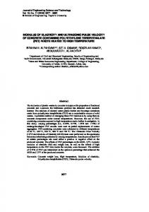
recommended to consider the temperature dependence, when the speed of sound is calculated by Equation 2.16. For example, a third order polynomial to model the temperature dependence of the adiabatic exponent κ can be used. The results of these calculations of the adiabatic exponent via these polynomials are also presented in Figure 2.2. Both polynomials κsto (T ◦C) and κair (T ◦C) for “stoichiometric” exhaust gas and dry air are given as follows: κsto (T ◦C) = 1.3751581−1.158914×10−4 T −3.1887584×10−8 T 2 +5.2602490×10−11 T 3 , (2.18) and κair (T ◦C) = 1.3993687−7.3729153×10−6 T −2.8499084×10−7 T 2 +2.5464712×10−10 T 3 . (2.19) The deviation away from the stoichiometric operation of the combustion engine, to the case where air is the main component in the exhaust gas, is also a reason that the speed of sound c changes its value. In the worst case, i.e. at 600 ◦ C and with λ = ∞, the speed of sound c would be calculated by a value of 9.89 m/s (1.73%) too small with the implicit understanding that the combustion is a stoichiometric one.

Speed of sound c [m/s]


600 580 560 540 520 500 480 460 440 420 400 380 360 340 320 300 -40 0

17

with constant adiabatic exponent κ(0°C) in dry air. with temperature dependent adiabatic exponent κ(T) in dry air.

with constant adiabatic exponent κ(0°C) at stoichiometric combustion. with temperature dependent adiabatic exponent κ(T) at stoichiometric combustion. 40 80 120 160 200 240 280 320 360 400 440 480 520 560 600

Temperature T [°C]

Figure 2.3: Speed of sound in the exhaust gas at stoichiometric combustion and in dry air calculated with Equation 2.16 using two different adiabatic exponents κ, i.e. constant and temperature-dependent.

Chapter 3 Determination of the Flow Rate This chapter contains a discussion of equations to determine the gas velocity and the speed of sound inside the flowmeter for different measurement pipe configurations. Both results are required for mass flow rate determination. It is demonstrated that the basic equations presented in Section 2.2 are not appropriate for the measurement pipe configuration utilized in this work (double-path flowmeter) for flowmetering in exhaust gas trains of combustion engines. The main drawback of these basic equations is that they do not consider transducer port cavities, which are inevitably present if the transducers are flushly-mounted in the measurement pipe. Further, if significant large flow velocities are expected, for example > 15% of the speed of sound, the sound drift effect should be taken into account for the calculation of the speed of sound. The value of the gas flow velocity obtained is not affected by this sound drift effect. Additionally, a special asymmetric pipe configuration which has its receiving transducers shifted in the direction of the flow is discussed, which requires its own set of equations. The major goal of this chapter is to provide all quantities for the equations to determine the volumetric flow rate and the mass flow rate which are required if the transit times tup and tdown are already determined (Chapter 7). Therefore, the determination of the meter factor which relates the sound-path-averaged gas velocity to the cross-sectional-averaged gas velocity is discussed in detail for both a centric and an eccentric measurement pipe configuration. Finding an appropriate model equation to describe the velocity distribution inside the measurement pipe is essential for the meter factor determination and therefore also for the flow rate calculation. Thus, the commonly used approaches to describe the gas velocity distribution are presented and compared directly. The last section provides the final equations and assumptions for calculation of the volumetric flow rate and the mass flow rate. These equations have been implemented in measurement software for the first realized measurements in the test bed environment (Chapter 8).

18

3.1. DERIVATION OF UFM EQUATIONS

3.1

19

Derivation of UFM Equations

As shown in Section 2.2 the commonly used equations for UFMs, i.e. Equation 2.5 and Equation 2.6, are only approximation equations. The main drawback of these equations is the fact that they do not consider the drift of the ultrasonic pulse due to the flowing gas and further they do not consider the influence of the transducer port cavities. The transducer port cavities exist if the transducers are flushly-mounted in the measurement pipe, which is advantageous due to the fact that the front part of the transducer is not directly located inside the hot main gas flow. Such a transducer port cavity can be seen in Figure 3.1(c) or 3.1(d). In general, this configuration is preferred if the transducers should be protected against the hot main gas flow. For example, in [8] flushly-mounted transducers are utilized for this reason. If the transducers are not flushly-mounted in the measurement pipe, half of the transducer membrane is located in the measurement pipe and the other half is located inside the transducer port cavity. For example, such a configuration is used in [18]. Here in this work, a configuration with flushly-mounted transducers is employed. The exact geometry of the measurement pipe and the transducer port cavities is presented in Section 4.2.1. Besides the transducer port cavities the sound drift should be considered by the equations too. The main goal of this section is to derive equations which eliminate or reduce the influence of the weak points of the basic equations which were derived in Section 2.2. Figure 3.1 is utilized for these derivations. In this context it should be noted that Figure 3.1 uses some simplifications. For example, the receiving (R) and transmitting (T) transducers are outlined using small points and the upstream and downstream channel is drawn separately only for reasons of clarity. The figure shows the six different situations which are distinguished in the next sections, i.e. 3.1.1 to 3.1.6.

3.1.1 Equations corresponding to Figure 3.1(a) As shown in Section 2.2 the two travel times of the ultrasonic pulses propagating upstream and downstream, i.e. tup and tdown , and the geometric parameters L and α (Figure 3.1(a)) are employed for determination of the gas flow velocity v and the speed of sound c. The equations obtained are tup − tdown L , (3.1) v= 2 sin (α) tup tdown and c=

L tup + tdown . 2 tup tdown

(3.2)

CHAPTER 3. DETERMINATION OF THE FLOW RATE

20 R

v

R

R

L, c

Flow

R

v tup

v

L, c

Flow

α

α

T

T

L, c

v tdown

α

α

L, c

T

T

(a)

(b)

Transducer Port Cavitiy

Transducer Port Cavitiy L0

L0

2

α

T0 , c0

2

α

T0 , c0

v

v

Flow

Flow

L − L0

α

α

L − L0

v tdown

(c) Δx

(d) R

Δx

γ

β L

v

L

Flow

Δx

R

L1

Δx

R

γ

β

L2

v

L

Flow

α

α

R

L1

v tdown

L2

v tup

α

α L

T

T

(e)

T

T

(f)

Figure 3.1: Schematics to explain the assumptions and considerations for the derivations of the equations from this section to determine the gas flow velocity v and the speed of sound c in a double-path flowmeter. The following situations are distinguished: (a) No sound drift; no transducer port cavities; (b) with sound drift; no transducer port cavities; (c) no sound drift; with transducer port cavities; (d) with sound drift; with transducer port cavities; (e) no sound drift, no transducer port cavities, with shifted receiving transducers; (f) with sound drift, no transducer port cavities, with shifted receiving transducers.


21

3.1.2 Equations corresponding to Figure 3.1(b) Due to the fact that the two ultrasonic pulses, propagating from the transmitting transducers to the opposite arranged receiving transducers, require a finite time to travel through the moving medium, both ultrasonic pulses are drifting in the direction of the flow. The theory of this drift effect is discussed in detail in Section 4.1.3. Concerning the magnitude directivity patterns (Figure 4.13) of the transducers utilized in the flowmeter, the following consideration can be made: Due to the sound drift effect, the part of the directivity pattern of the transducer that arrives at the receiver location originates from a part of the directivity pattern differing from the maximum at the angle Θ = 0. The ultrasonic pulse propagating in the downstream channel of the flowmeter is affected during the time period tdown by the flowing gas. Therefore, this ultrasonic pulse moves the distance v tdown in the direction of the flow. In the upstream channel the ultrasonic pulse is affected during the time period tup which results in a superimposed movement of the distance v tup , also in the direction of the flow. In both situations, outlined in Figure 3.1(b), the relations

2 c2 − L2 cos2 (α) + v tdown (3.3) L sin (α) = tdown for the downstream channel of the flowmeter, and

2 c2 − L2 cos2 (α) − v t L sin (α) = tup up

(3.4)

for the upstream channel of the flowmeter are obtained. These relations can be solved for the gas flow velocity v and the speed of sound c, which results in v=

tup − tdown L , 2 sin (α) tup tdown

which is exact the same result as represented by Equation 3.1, and tup − tdown 2 L 4 1 c= + . 2 2 sin (α) tup tdown tup tdown

(3.5)

(3.6)

This result shows that considering the sound drift in the derivation of the equations for v and c only affects the speed of sound c. Equation 3.6 is equal to results reported in [15, 19]. In comparison to Equation 3.2, Equation 3.6 yields a more precise result, especially when the gas velocity, and therefore the sound drift effect, is high. Equation 3.2 delivers a speed of sound c which is too small. However, the difference is only significant when the determined travel time difference Δt = tup − tdown is large. For example, for a measurement pipe configuration with L = 65.24 mm and α = 30◦ and an assumed travel time of 200 µs for zero flow velocity, the difference in the speed of sound calculated with Equation 3.2 and 3.6 respectively is approximately 0.84% for a travel time difference Δt = 30 µs. Thus, Equation 3.6 is recommended instead of Equation 3.2 for determining of the speed of sound c.


22

3.1.3 Equations corresponding to Figure 3.1(c) The transducers are flushly-mounted in the measurement pipe, which results in transducer port cavities. Depending on the diameter of the transducers used, a specific diameter for the transducer port is required. Further, the sound path angle α has an influence on the average depth of the transducer port cavity. Figure 3.1(c) shows the conditions concerning the transducer port cavity. In Figures 3.1(a) and 3.1(b), L labels the distance between the opposite arranged transducers, which is also the case for Figure 3.1(c). However, due to the transducer port cavity with the average depth L0 2 the effective distance on which the ultrasonic pulse is fully influenced by the main gas flow is reduced to L − L0 . This is also the case if the ultrasonic pulse does not propagate exactly at the connecting line from the transmitting transducer to the receiving transducer, due to the symmetry concerning the opposite arranged transducer port cavity which also has the average depth L0 2. If the ultrasonic pulse propagates parallel to the connecting line, also shown in Figure 3.1(c), the length of the path on which the ultrasonic pulse is inside the transducer port cavity is always the same. This is essential for the derivation of the equations for determining the gas flow velocity v and the speed of sound c. If the transducer port cavity diameter is small in comparison to the pipe diameter of the measuring pipe itself, the temperature T0 inside the transducer port cavity is almost equal to the wall temperature Tw . Inside the transducer port cavity the gas velocity is low and there exists a flow vortex. One can argue that this vortex is partially surrounded by the wall of the measurement pipe, which is at the temperature Tw , and therefore T0 ≈ Tw . This will be discussed in Chapter 4. Knowledge of the temperature inside the transducer port cavity can be utilized for the derivation of the required equations for v and c. As shown in Section 2.3 the temperature information T0 , which for example can be obtained from a temperature sensor located inside the transducer port cavity, can be used for the calculation of the speed of sound c0 . This value is only valid for the range inside the transducer port cavities. Using the value c0 leads to write the relations tdown =

L0 L − L0 + c + v sin (α) c0

(3.7)

for the downstream channel and tup =

L0 L − L0 + c − v sin (α) c0

(3.8)

for the upstream channel. The concept of this approach is that the upstream and down stream travel times are increased by the amount L0 c0 due to the fact that compared to the case from Section 3.1.1 the ultrasonic pulse also has to propagate through two transducer port cavities with the overall average depth L0 . Further, when using this approach it is assumed that the ultrasonic pulse is only affected on the path L − L0 inside the measurement pipe by the gas flow velocity v. Solving these relations for the gas flow velocity v and the speed of sound c results in v=

(tup − tdown ) (L − L0 ) c20 1 , 2 sin (α) (L0 − c0 tup ) (L0 − c0 tdown )

(3.9)


23

and

1 (c0 tup + c0 tdown − 2 L0 ) (L − L0 ) c0 . (3.10) 2 (L0 − c0 tup ) (L0 − c0 tdown ) The ratio between Equation 3.9 and 3.1, and the ratio between Equation 3.10 and 3.2 is helpful for the demonstration of the influence of the transducer port cavities. Equation 3.9 divided by Equation 3.1 gives c=

(L − L0 ) c20 tup tdown vPort = , vBasic (L0 − c0 tup ) (L0 − c0 tdown ) L

(3.11)

and Equation 3.10 divided by Equation 3.2 gives (c0 tup + c0 tdown − 2 L0 ) (L − L0 ) c0 tup tdown cPort = . cBasic (L0 − c0 tup ) (L0 − c0 tdown ) L (tup + tdown )

(3.12)

Figure 3.2 visualizes the result of Equation 3.11 and Equation 3.12 for concrete values, for two different averaged gas temperatures, i.e. 20 ◦ C and 600 ◦ C. The geometric parame1,132

1,005

20°C 600°C

1,130 1,129 1,128 1,127 1,126 -30µ

-20µ

-10µ

0

10µ

20µ

Travel time difference Δ t [s]

20°C 600°C

1,004

Ratio cport / cbasic

Ratio vport / vbasic

1,131

30µ

1,003 1,002 1,001 1,000 -30µ

-20µ

-10µ

0

10µ

20µ

30µ

Travel time difference Δ t [s]

(a)

(b)

Figure 3.2: (a) Ratio between results obtained from Equations 3.9 and 3.1, and (b) ratio between results obtained from Equations 3.10 and 3.2. ters for Figure 3.2 are L= 65.24 mm and L0 = 7.5 mm. Concerning the two temperatures 20 ◦ C and 600 ◦ C, for c0 the values used are 343 m/s and 580 m/s respectively. These values correspond to the mean travel times tm = 195.33 µs and tm = 115.51 µs, which were used for approximation of the required travel times tup and tdown for the Equations 3.11 and 3.12. Figure 3.2 shows that the influence of the transducer port cavities is significant for the determined values of the gas flow velocity in contrast to the speed of sound. Further, it shows that at elevated temperatures the influence is more significant.

3.1.4 Equations corresponding to Figure 3.1(d) The results for v and c obtained in Sections 3.1(a) and 3.1(b) showed a significant difference concerning the speed of sound c. Thus, the sound drift effect and the transducer

24


port cavities are taken into account for the following derivation. Figure 3.1(d) shows the conditions for one transducer port cavity when the sound drift effect should be considered too. A modification of the Equations 3.3 and 3.4, similar to that discussed in Section 3.1.3, results in L0 2 2 L0 2 2 tdown − (3.13) c − (L − L0 ) cos (α) + v tdown − (L − L0 ) sin (α) = c0 c0 for the downstream channel of the flowmeter, and L0 2 2 L 0 2 (L − L0 ) sin (α) = c − (L − L0 ) cos2 (α) − v tup − tup − c0 c0

(3.14)

for the upstream channel. Solving these relations for the flow velocity v and for the speed of sound c yields (tup − tdown ) (L − L0 ) c20 1 v= , (3.15) 2 sin (α) (L0 − c0 tup ) (L0 − c0 tdown ) the exact same result as shown in Section 3.1.3, and

4 (L0 − c0 tup ) (L0 − c0 tdown ) sin2 (α) + (tdown − tup )2 c20 (L − L0 ) c0 1 . c= 2 sin (α) (L0 − c0 tup ) (L0 − c0 tdown ) (3.16) Due to the fact that Equation 3.16 also considers the sound drift effect, the results obtained is more precise in comparison to the result obtained from Equation 3.10. For example, for a measurement pipe configuration with L = 65.24 mm, L0 = 7.5 mm, and α = 30◦ the difference between the results is approximately 1.1% for a 20 ◦ C gas temperature and 3.1% for a 600 ◦ C gas temperature, if a travel time difference Δt = 30 µs is the underlying assumption.

3.1.5 Equations corresponding to Figure 3.1(e) Figure 3.1(e) shows a special double-path flowmeter configuration which has its receiving transducers shifted in the direction of the flow. The concept of this configuration is that shifting both receiving transducers in the direction of the flow partially compensates the sound drift effect which inevitably reduces the receiving amplitudes in both channels (Section 4.3). So, the major goal of this configuration is a larger measurement range. This configuration is numerically investigated in Section 4.3.5. The drawback of this configuration is its asymmetry. However, an analytical solution for the gas flow velocity v and the speed of sound c can be found, if the value Δx is known (Figure 3.1(e)). A further drawback is the fact that there is no optimum shift for different operating conditions of the UFM. An adaptive adjustable flowmeter configuration can be used to overcome this problem. Figure 3.3 shows a feasible UFM which has this feature included, i.e. the two receiving transducers can be shifted with or against flow direction during operation.


25

Figure 3.3: Design drawing of a measurement pipe which enables to shift both receiving transducers by the same amount Δx with or against the flow direction. (Drawing by courtesy of AVL List Ges.m.b.H.). Concerning the situation outlined in Figure 3.1(e) the relations L1 tdown

= c + v sin (β)

(3.17)

for the downstream channel of the flowmeter, and L2 = c − v sin (γ) tup

(3.18)

for the upstream channel can be written, which are similar to the approach employed in Section 2.2. Equations 3.17 and 3.18 can be solved for v and c and substitution of the expressions L sin (α) + Δx , (3.19) sin (β) = L1 and L sin (α) − Δx (3.20) sin (γ) = L2 into this solution gives v= tup tdown and c=

t L −t L up 1 down 2 , L sin(α)+Δx L sin(α)−Δx + L1 L2

t L (L sin(α)−Δx) tdown L2 (L sin(α)+Δx) + up 1 L2 L1 . L sin(α)−Δx tup tdown L sin(α)+Δx + L1 L2

(3.21)

(3.22)


26

In Equations 3.21 and 3.22 all information is included which is required for calculation of v and c. In this context it should be noted that the two distances L1 and L2 between the receiving and transmitting transducers can be determined using the equations L1 = and L2 =

Δx2 + L2 + 2 Δx L sin (α),

(3.23)

Δx2 + L2 − 2 Δx L sin (α).

(3.24)

3.1.6 Equations corresponding to Figure 3.1(f) Similarly as described in Section 3.1.2 the sound drift effect can be considered, if the receiving transducers are shifted in the direction of the flow. This situation is outlined in Figure 3.1(f). Again the relations L1 sin (β) =

2 tdown c2 − L2 cos2 (α) + v tdown ,

(3.25)

2 c2 − L2 cos2 (α) − v t tup up

(3.26)

and L2 sin (γ) =

can be solved for v and c, which gives

2 2 2 − L2 sin2 (γ) t 2 + L12 sin2 (β) tup − tdown 1 L2 cos2 (α) tup 2 down v= 2 tdown tup (L1 sin (β) tup + L2 sin (γ) tdown )

(3.27)

for the gas flow velocity, and √ AB 1 c= 2 tdown tup (L1 sin (β) tup + L2 sin (γ) tdown )

(3.28)

for the speed of sound, where A and B are abbreviations for the expressions A = L2 cos2 (α) (tup − tdown )2 + (L2 sin (γ) tdown + L1 sin (β) tup )2 ,

(3.29)

B = L2 cos2 (α) (tup + tdown )2 + (L2 sin (γ) tdown + L1 sin (β) tup )2 .

(3.30)

and

The geometric parameters required for Equations 3.27 and 3.28 again can be calculated by using Equations 3.19, 3.20, 3.23, and 3.24.

3.2. DETERMINATION OF THE METER FACTOR

3.2

27

Determination of the Meter Factor

A fundamental problem in acoustic flow measurement is the fact that the distribution of the velocity in the measurement pipe in each case is not known exactly. In the case of an acoustic transit-time flowmeter this plays a major role, because an ultrasonic transittime flowmeter always determines the averaged velocity along the sound path (vP ), i.e. an ultrasonic flow meter integrates the velocity profile over the volume of the sound beam. However, the velocity required for computing the volumetric flow rate Qv is the flow velocity vA , the averaged velocity over the cross-sectional area of the pipe, as shown in Equation 2.1. Exact knowledge of the velocity profile is essential to convert the lineaveraged path velocity vP to the velocity vA . The connection between these two velocities vP and vA is usually considered by a correction factor kv , also termed meter factor [7]: kv =

vA . vP

(3.31)

The basis for different approaches of modelling the velocity profiles are usually undisturbed axially symmetric flow profiles in circular pipes. The analysis of the influence of disturbed flow profiles to the meter factor kv is presented in [39, 40, 41]. The influence of swirl and cross flow is investigated in e.g. [42]. In this work an axially symmetric flow profile is assumed. Through a sufficiently long starting and stopping length before and after the crossed sound paths, one tries fulfill this condition. Additionally, a flow conditioner can be used [43, 44, 45]. In the simplest case a flow conditioner consists of a bundle of small pipes inside the starting length before the ultrasonic flow meter (Section 8.1). In e.g. [25] for the lower limit of the starting length to obtain a roughly axially symmetric flow profile the specification 10D, i.e. ten times the pipe diameter, can be found. The lower limit for the stopping length is given by 5D. However, these guide values do not guarantee a completely developed axially symmetric flow profile, and are a compromise between a usable size of the flowmeter and an additional error source1 . The meter factor kv (Equation 3.31) can be calculated easily for a given axially symmetric flow profile v(r), where r denotes the radius. The flow profile v(r) related to the crosssectional area A of the pipe must be averaged to determine vA , i.e. 1 vA = A

R

v (r) dA (r),

(3.32)

0 1 Considerably longer starting and stopping lengths are required to be able to guarantee a completely developed axially symmetric flow profile. According to [46] a starting length of ≈ 50D would be required for the flowmeter. In [47] the influence of two pipe configurations, a single-elbow and a double-elbow configuration, located 10D before an ultrasonic flowmeter, is investigated. In [47] the tests were made for reference conditions of 100D straight-pipe configurations to ensure a fully developed flow profile at the entrance of the flowmeter.


28

where R is the radius of the pipe. On the basis of the assumed axial symmetry the integration over half of the pipe diameter, i.e. the radius R, is sufficient. An appropriate substitution gives 2 vA = 2 R

R

v (r) r dr.

(3.33)

0

Concerning the calculation of the line-averaged path velocity vP one must distinguish between an eccentric and a centric arrangement of the sound paths. In Figure 3.4 both cases are presented. In each case, a) and b), only one sound path with the transducer positions 1 and 2 is shown. Further, a schematic representation of the assumed axially symmetric flow profile v(r) is also shown. In the eccentric case b) the sound path has an offset h from the center of the pipe, so the distance between the transducers reduces from radius R to the distance b. Due to the assumed axial symmetry of the flow profile v(r) y 2

2 v (r)

z

x

1

1 (a)

y 2

2

h r

v (r)

z

x s

1

1 (b)

Figure 3.4: Schematic representation of a sound path under an angle α: a) Centric arrangement, and b) eccentric arrangement in the level distance h.

the integration over half of the covered distance of the ultrasound is again sufficient. It should be noticed that the angle α between the sound path and the cross-sectional area

3.2. DETERMINATION OF THE METER FACTOR

29

of the pipe has no influence on the value of this averaging. Hence the line-averaged path velocity vP for the centric case is calculated by the following equation 1 vP = R

R

v (r) dr.

(3.34)

0

Substituting Equations 3.33 and 3.34 into Equation 3.31 leads to the meter factor kv for the centric arrangement of the sound path:

R

v (r) r dr vA 4 0 kv = = . vP D R v (r) dr

(3.35)

0

Equation 3.35 shows clearly that the meter factor kv depends directly on the flow profile v(r). Each deviation of the flow profile from the assumed one, which is used in Equation 3.35, forcibly leads to uncertainties of the flowmeter. Finding an appropriate model equation for the flow profile v(r) for each flow measurement problem is essential. A comparison of different approaches for flow profile modelling is discussed in Section 3.3. In the case of an eccentric sound path arrangement (Figure 3.4(b)), the meter factor kv also depends on the flow profile in the pipe. The calculation of kv necessitates an integration over the sound path to obtain the path averaged velocity vP , i.e. for the eccentric case, vP is calculated similarly to Equation 3.34: 2 b

1 1 2 2 (3.36) v (r) ds = v h + (b − s) ds, vp = 2b b 1

0

where v(r) again is the representation of the axially symmetric flow profile in the measurement pipe. Substituting Equations 3.33 and 3.36 into Equation 3.31 leads to the meter factor kv for the eccentric arrangement of the sound path: vA kv = = vP

2 R2

1 b

b

v

R

v (r) r dr

0

.

2

h2 + (b − s)

(3.37)

ds

0

The eccentric sound path arrangement gives the possibility of selecting an appropriate level h, so that the influence of the degree of flow turbulence on the meter factor kv is minimized. In that case, Equation 3.37 is the initial equation. A detailed analysis of this can be found in [25], where an optimum level the value of h/R is found to be approximately 0.4. Generally, the eccentric sound path arrangement is commonly used for all large-sized pipe diameters, that is those with D ≥ 150 mm. In the case of ultrasonic flow metering in hot gases (e.g. exhaust gas), two main reasons exist where it is not useful to use an eccentric sound path arrangement. These reasons are:

30

CHAPTER 3. DETERMINATION OF THE FLOW RATE 1. In exhaust gas trains of automotive combustion engines, pipe diameters bigger than 120 mm are very rare. In this context only large-displacement motors are an exception. Eccentric sound path arrangements are impractical for pipe diameters smaller than 150 mm, due to their finite transducer geometry [25]. The same applies to the usage of several sound paths next to each other [7]; 2. In an exhaust gas train, steep temperature gradients between the pipe wall and the center of the pipe may occur. Therefore, the eccentric sound path arrangement has the drawback of a larger deviation from its original sound path without a temperature gradient, as compared to the centric sound path configuration. Hence, the acoustic waves are refracted toward the colder areas in the pipe and therefore, away from the ideal path to the receiving transducer, which limits the measurement range (Section 4.3.5).

An appropriate model equation for the flow profile v (r) must be employed to determine the required meter factor kv for the centric or eccentric sound path arrangement. The first step to find such a model equation is to characterize the type of the flow inside the pipe, which can be characterized as being laminar, turbulent, or something in between called transitional [6]. The type of a fluid flow can be characterized for a wide range of conditions by the non-dimensional Reynolds number Re, defined by Re =

vA D , ν

(3.38)

where vA is again the average velocity over the pipe cross-sectional area, D is the pipe diameter, and ν is the kinematic viscosity of the gas (e.g.: ν = 4.809 × 10−5 m2 /s for dry air at 300 ◦ C and 1 bar [35]). Generally, the Reynolds number Re is a stability criteria for laminar fluid flows. Empirical limit values (critical Reynolds number Recrit ) can be found for different geometries. In circular pipes, turbulent flows are encountered when Re > 4000 [48, 25] and laminar flows are encountered when Re < 2000 ([49]) or Re < 2300 [50, 51]. In flow systems design, operation in the transitional flow regime should be avoided. Equation 3.38 facilitates the estimation of the range of the Reynolds numbers, which occur in an exhaust gas train for an automotive combustion engine. Concerning the diagram in Figure 3.5 the following assumptions were made: the pipe diameter is D = 50 mm and the kinematic viscosity ν of the gas is in the range 1.3 × 10−5 . . . 9.6 × 10−5 m2 /s, which corresponds to a temperature range from 0 . . . 600 ◦ C for dry air at a pressure of 1 bar. Figure 3.5 shows that the temperature has a strong influence on the lower velocity limit vA of the flow, i.e. when the flow starts to be fully turbulent. In the worst case, i.e. at an assumed upper gas temperature limit of 600 ◦ C, a flow velocity vA of approximately 8 m/s is necessary. Further, an exhaust gas flow of a combustion engine has the peculiarity that the gas flow is superposed by pulsating pressure fluctuations. These superpositions are generated by the pistons of the combustion engine, which push the exhaust gas periodically into the exhaust gas train. The level of turbulence of this gas coming from the

3.3. MODEL EQUATIONS TO DESCRIBE THE VELOCITY DISTRIBUTION

31

5000

Reynoldsnumber Re

4500 4000 3500 3000 2500 2000 1500 1000

2

ν = 1.3 e-5 [m /s], 0°C

500

2

ν = 9.6 e-5 [m /s], 600°C

0 0

1

2

3

4

5

6

7

8

9

10

Cross sectional averaged velocity vA [m/s]

Figure 3.5: Reynolds numbers for dry air in a Ø50 mm circular pipe at a pressure of 1 bar. Calculated for 0 ◦ C (ν = 1.3 × 10−5 m2 /s) and for 600 ◦ C (ν = 9.6 × 10−5 m2 /s).

combustion chamber is very high, so one may assume that the flow in the exhaust gas train is completely turbulent. This is also the case for Reynolds numbers smaller than 4000. In [15] it was shown that the flow is turbulent irrespective of the engine speed. Hereinafter a fully developed turbulent flow profile in the exhaust gas train is assumed, whereby one has to take into account that there exist several formulae to describe the velocity profile mathematically.

3.3

Model Equations to describe the Velocity Distribution

The following three Sections 3.3.1 to 3.3.3 deal with the commonly used formulae for radially symmetric velocity profiles, whereby smooth walled circular pipes are the underlying assumption. In Section 3.3.4 these formulae are compared directly.

3.3.1 Power Law The first often used formula is given by v (r) = vmax

r 1n 1− R

(3.39)

32


with n = f (Re), where vmax is the maximum flow velocity in the center of the pipe, r is the distance from the center of the pipe in radial direction and R is the radius of the pipe. This formula is known under various names. In [25] it is called “Power Law,” in [48] one can find the name “turbulent pipe profile” and in [52] it is called the “fully developed velocity profile.” Generally, the formula given by Equation 3.39 is often used in industrial applications. A large number of empirical relations can be found in literature [7, 25, 52, 48] for the Equation n = f (Re). In [25] some empirical relations for n = f (Re) from different authors are compared directly in the range 4000 < Re < 2 × 106 . The equations considered are n1 = 11.269 − 3.019 log10 Re + 0.432 log210 Re, n2 =

1 , 0.25 − 0.023 log10 Re

(3.40) (3.41)

and n3 = 2.25 log10 Re − 2.85.

(3.42)

Equation 3.41 is also used in [48] for a numerical simulation of an ultrasonic transit-time flowmeter. In [7] for n = f (Re) the equation n4 = 1.66 log10 Re

(3.43)

can be found, and in [52], for the case of a smooth walled pipe the implicit equation, Re n5 = 2 log10 − 0.8 (3.44) n is used. A clear comparison of these five relations for n = f (Re) (Equations 3.40 to 3.44) is presented in Figure 3.6. In Figure 3.6(a) a range for the Reynolds number beginning at 4000 and ending at 192307 was used. According to Equation 3.38 this corresponds to a velocity range of 1 . . . 50 m/s for vA , when dry air at a temperature of 0 ◦ C flows in a Ø50 mm circular pipe. In Figure 3.6(b) the value for the Reynolds number Re also begins at 4000 but ends at 26041, which again corresponds to a velocity range of 1 . . . 50 m/s (Figure 3.5) for dry air at a temperature of 600 ◦ C flowing through the pipe. A direct comparison of both diagrams in Figures 3.6(a) and 3.6(b) show that the values for n decrease as the temperature of the fluid increases. The average of all values for n is calculated by different equations. In the visible range in Figure 3.6(a) the average is 7.387, at a standard deviation of 0.548. In Figure 3.6(b) the average is 5.358 at a standard deviation of 0.291. In applications where ν, that is the kinematic viscosity of the gas, is treated as constant the most commonly used value for n in the Power Law (Equation 3.39) is 7. In this context the Power Law has been named the “1/7-Power-Law” [50, 53, 54, 55, 15]. This is in good agreement with the averaged values for n in a lower temperature range. In applications such an ultrasonic flowmeter for exhaust gas, ν cannot be treated as constant due to the wide temperature range. It can be calculated from temperature, pressure

10,0 9,5 9,0 8,5 8,0 7,5 7,0 6,5 6,0 5,5 5,0 4,5 4,0 3,5 3,0 1

5

10

15

20

25

n1

n2

n4

n5

30

35

40

n3

45

Cross-sectional averaged velocity vA [m/s]

50

Different n for Power Law at 600°C

Different n for Power Law at 0°C


(a) 0 ◦ C.

10,0 9,5 9,0 8,5 8,0 7,5 7,0 6,5 6,0 5,5 5,0 4,5 4,0 3,5 3,0 8 10

n1

n2

n4

n5

15

20

33

n3

25

30

35

40

45

50


(b) 600 ◦ C.

Figure 3.6: Comparison of results from different calculation methods (Equation 3.40 to 3.44) for the value n in the Power Law (Equation 3.39) for a dry air flow at 0 ◦ C (a) and at 600 ◦ C (b) in a Ø50 mm pipe.

or viscosity data, or it can be calculated from the speed of sound, as an indicator of temperature or viscosity [7]. The latter is particularly interesting for transit-time ultrasonic gas flowmeters, due to its ability to determine the speed of sound (Section 2.3).

1,1 1,0 0,9 0,8 0,7 0,6 0,5 0,4 0,3 0,2 0,1 0,0

kv

v/vmax

Figure 3.7(a) shows several normalized velocity profiles calculated by the Power Law with different values for n. In the Figures 3.6(a) and 3.6(b), for n, the range starting from 5 and ending at 9 is selected. Figure 3.7(a) shows a specific feature, which is typical of

n=5 n=6 n=7 n=8 n=9 -1,0 -0,8 -0,6 -0,4 -0,2 0,0 0,2 0,4 0,6 0,8 1,0

0,96 0,95 0,947 0,94 0,933 0,93 0,92 0,91 0,909 0,90 0,89 0,88 0,87 0,86 0,85 0,84 3,0 3,5 4,0 4,5 5,0 5,5 6,0 6,5 7,0 7,5 8,0 8,5 9,0 9,5 10,0

r/R

(a)

n

(b)

Figure 3.7: (a) Normalized velocity profiles by the Power Law (Equation 3.39) with different values for n. (b) Meter Factor kv (Equation 3.35) calculated for velocity profiles by the Power Law (Equation 3.39) with different values for n.

34


the Power Law formula. At r = 0, i.e. in the center of the pipe, the first derivation of the Power Law shows a discontinuity. From physical considerations one may expect that dv (r) = 0, (3.45) dr r=±0 which is definitely not the case when the Power Law is used to model the distribution of the velocity of the gas flow. The Power Law does not represent the velocity distribution in the center of the pipe satisfactorily. If smaller values for n are substituted into Equation 3.39 this discontinuity becomes more significant. Using the Power Law (Equation 3.39) and Equation 3.35 for the centric sound path arrangement, concrete values for the meter factor kv , dependent on the value n can be determined. The result of these calculations are presented in Figure 3.7(b). The level of turbulence, i.e. the concrete value for n, should not treated as constant.

3.3.2 Parabolic Law An additional approach, which is also analyzed in [25], is given by r 2 m , v (r) = vmax 1 − R

(3.46)

with m = f (Re), similar to Equation 3.39. This approach is called the “Parabolic Law,” because it is based on the well known parabolic velocity profile for fully developed laminar pipe flows, which can be deduced from the Navier-Stokes equations [56]. This velocity profile is given by r 2 , (3.47) v (r) = vmax 1 − R that is, Equation 3.46 with m = 1 [57]. According to [25], this approach describes the fully developed turbulent velocity profile if m > 5. Similar to the empirical relations for n = f (Re) there also exists an empirical relation for m = f (Re) for the Parabolic Law [25]: 0.8741 + 0.0121 log10 Re . (3.48) m= 2 (0.1259 − 0.0121 log10 Re) In the same way as for the Power Law, one can find a range for m using Equation 3.48. The assumptions are again two gas temperatures which are the lower and upper limits, 0 ◦ C and 600 ◦ C respectively. Figure 3.8 shows the possible range for m. At a 600 ◦ C gas temperature, the critical Reynolds number Re = 4000 until a flow velocity vA of 8 m/s is reached. Again a pipe diameter of D = 50 mm is assumed. The advantage of the Parabolic Law is its ability to describe both laminar and turbulent fluid flow. Hence, the dashed part of the lower curve in Figure 3.8 can be described by the Parabolic Law. The range of values of m for the application of flow measurement with the assumptions described

m for Parabolic Law at 0°C and 600°C


35

8,0 7,5 7,0 6,5 6,0 5,5 5,0

0°C 600°C 1

5 8 10

15

20

25

30

35

40

45

50


Figure 3.8: Visualization of the value m (Equation 3.48) for the Parabolic Law (Equation 3.46) at 0 ◦ C and 600 ◦ C for different gas velocities in a circular (D = 50 mm) pipe.

1,00

1,1 1,0 0,9 0,8 0,7 0,6 0,5 0,4 0,3 0,2 0,1 0,0

0,95

0,942 0,916

0,90

kv

v/vmax

above is from 5 to 7.6. Figure 3.9(a) shows several normalized velocity profiles calculated by the Parabolic Law with different values of m. The velocity profile for the laminar gas flow (m = 1), given through Equation 3.47, is also presented in this figure. Similar to the

m=1 m=5 m=6 m=7 m = 7.5

0,85 0,80 0,75 0,70

-1,0 -0,8 -0,6 -0,4 -0,2 0,0 0,2 0,4 0,6 0,8 1,0

1

2

3

4

5

r/R

(a)

6

7

8

9

10

m

(b)

Figure 3.9: (a) Normalized velocity profiles determined by the Parabolic Law (Equation 3.46) with different values for m. (b) Meter Factor kv (Equation 3.35) calculated for velocity profiles by the Parabolic Law (Equation 3.46) with different values for m.

Power Law, the meter factor kv dependent on m can be calculated with the Parabolic Law. Substituting Equation 3.46 into 3.35 and varying m in the range from 1 . . . 10 gives the curve presented in Figure 3.9(b).


36

3.3.3 Logarithmic Law The last formula to describe the velocity profile v(r) discussed in this chapter is the socalled “Logarithmic Law.” In contrast to the Power Law and the Parabolic Law (Equations 3.39 and 3.46) the Logarithmic Law is not valid in the immediate vicinity of the pipe wall [25]. It is given by the equation r , (3.49) v (r) = vmax 1 + q ln 1 − R where the abbreviation q is given by [25]: vτ log10 (e) , (3.50) q = 5.65 vmax where vτ is the shear stress velocity. In the case of the Logarithmic Law it is helpful to determine the relation between the cross-sectional averaged velocity vA and the maximum velocity vmax in the center of the pipe. Substituting Equation 3.49 into Equation 3.33 and dividing by vmax delivers vA = vmax

2 R2

R 0

vmax 1 + q ln 1 − Rr r dr vmax

= 1−

3 q, 2

(3.51)

which enables one to express the maximum velocity vmax with the aid of Equation 3.50 in the form 3 (3.52) vmax = vA + 5.65 vτ log10 (e) . 2 Substituting Equation 3.52 into Equation 3.50 gives an explicit equation, which allows the calculation of q using the velocity vA and the shear stress velocity vτ . The same is also applicable when Equations 3.52 and 3.50 are substituted into Equation 3.49. The shear stress velocity vτ in Equation 3.50 can be calculated using the wall shear stress τ0 and the density ρ of the fluid by τ0 . (3.53) vτ = ρ The pipe wall causes a flow resistance, which affects the flowing fluid directly [56], i.e. the fluid flowing near to the pipe wall is delayed. In turbulent pipe flows there exists a thin fluid film in the immediate vicinity of the pipe wall. In this fluid film, which is termed the viscous sublayer, the viscous shear stress is much smaller than the turbulent shear stress. The definition of the dimensionless coefficient of friction λ, from Darcy-Weisbach, says that λ is four times the ratio of the wall shear stress τ0 and the dynamic pressure at the cross-sectional averaged velocity vA , i.e. τ0 λ≡4 2 . (3.54) ρ vA 2

The shear stress velocity vτ can be determined as follows: λ vτ = vA , 8

(3.55)


37

whereby the dimensionless coefficient of friction λ generally depends on the Reynolds number Re and on the roughness of the pipe wall. Similar to the Power Law and the Parabolic Law, one must estimate the cross-sectional averaged velocity vA to determine the Reynolds number Re (Equation 3.38). The dimensionless coefficient of friction λ depends on the Reynolds number Re and the relative roughness ks/D, where ks is the roughness of the pipe wall in mm. The coefficient of friction λ in turbulent pipe flows was empirically determined by many measurements over a large range of values for the Reynolds number Re and the relative roughness. The results of these measurements are summarized in diagrams, e.g. from Moody/Colebrook [36] and from Colebrook/Nikuradse [55]. Typical values for the roughness of the pipe wall ks can be taken from appropriate tables [55]. Concerning the following considerations a value ks = 0.001 mm for the roughness of the pipe wall (also called sandroughness) is assumed, which gives a value of 2 × 10−5 for the relative roughness when the pipe diameter D is 50 mm. In the Moody/Colebrook diagram this value lies in the area which indicates a hydraulically smooth pipe wall, i.e. the surface irregularities of the pipe wall lay completely lying within the viscous sublayer. In the case of hydraulically smooth pipes the dimensionless coefficient of friction λ only depends on the Reynolds number Re. This can be calculated by an empirical law, which is given by an implicit Equation 3.56 or by an accompanying approximate formula 3.57. These equations are [55]: √ Re λ 1 √ = 2.0 log , (3.56) 2.51 λ and 0.309 λ = 2 . log Re 7

(3.57)

In the diagrams in Figures 3.10 to 3.11, the cross-sectional averaged velocity vA is again treated as the input parameter. In the range vA = 1 . . . 50 m/s the Reynolds number Re for a specific fluid temperature is calculated using Equation 3.38. Again a value of D = 50 mm is assumed for the pipe diameter. Using Equation 3.56 or Equation 3.57 enables one to determine the dimensionless coefficient of friction λ for the pipe. Then substituting λ into Equation 3.55, using Equation 3.52, yields the required result for the abbreviation q (Equation 3.50), which can then be used for the calculation of the velocity profile given by Equation 3.49. The result of the calculated values of q, dependent on the velocity vA , is shown in the diagram in Figure 3.10. Again, both are for fluid temperatures 0 ◦ C and 600 ◦ C, as the lower and upper limits. The range of q, in the case of flow metering in an exhaust gas train, is between 0.1793 and 0.0936. Figure 3.11(a) shows several normalized velocity profiles calculated via the Logarithmic Law with different values for q. With increasing Reynolds numbers, i.e. with decreasing values for q, the flow profile becomes wider. Just as for the Power Law and the Parabolic Law, a meter factor kv (Equation 3.35) can also be calculated for the Logarithmic Law. Figure 3.11(b) shows the result of this calculation, i.e. kv dependent on q.


38

q for Logarithmic Law

0,30 0°C 600°C

0,25 0,20 0,15 0,10 0,05

0

5

10

15

20

25

30

35

40

45

50


1,00

1,1 1,0 0,9 0,8 0,7 0,6 0,5 0,4 0,3 0,2 0,1 0,0

0,95 0,90

kv

v/vmax

Figure 3.10: Visualization of the value q (Equation 3.50) for the Logarithmic Law (Equation 3.49) at 0 and 600 ◦ C for different gas velocities in a circular (D = 50 mm) pipe.

0,85 q = 0.1793 q = 0.1507 q = 0.1221 q = 0.0936 -1,0 -0,8 -0,6 -0,4 -0,2 0,0 0,2 0,4 0,6 0,8 1,0

0,80 0,75 0,30 0,28 0,25 0,23 0,20 0,18 0,15 0,13 0,10 0,08

q

r/R

(a)

(b)

Figure 3.11: (a) Normalized velocity profiles given by the Logarithmic Law (Equation 3.49) with different values for q. (b) Meter Factor kv (Equation 3.35) calculated for velocity profiles with the Logarithmic Law (Equation 3.49) for different values of q.

3.3.4 Comparison of the Power, Parabolic and Logarithmic Laws In this section the three formulae from Sections 3.3.1 to 3.3.3 for describing the flow distribution are compared. The diagram in Figure 3.12 directly compares the Power, Parabolic and Logarithmic Laws. The assumptions for this diagram are dry air at 25 ◦ C, a cross-sectional averaged velocity vA = 20 m/s and a pipe diameter D = 50 mm. These assumptions correspond to a value for the Reynolds number Re of 64000. Equation 3.42 was used to find an appropriate value for n for the calculation of the velocity profile via the Power Law, due to the fact that this equation is in best agreement with the Logarithmic


39

v/vmax

Law in the considered range of Reynolds numbers. Evident in Figure 3.12 is the strong 1,1 1,0 0,9 0,8 0,7 0,6 0,5 0,4 0,3 0,2 0,1 0,0

Power Law (n = 7.96) Parabolic Law (m = 6.88) Logarithmic Law (q = 0.1031) -1,0 -0,8 -0,6 -0,4 -0,2 0,0 0,2 0,4 0,6 0,8 1,0

r/R

Figure 3.12: Comparison of the normalized velocity profiles by the Power, Parabolic and Logarithmic Laws (Equations 3.39, 3.46 and 3.49) for an averaged velocity vA of 20 m/s (dry air at 25 ◦ C, pipe diameter D = 50 mm, Reynolds number Re = 64000). divergence of the result from the Parabolic Law in comparison to the other formulae, although it is recommended in [25]. In [58] pipe flows were measured using Laser Doppler Velocimetry (LDV). These results are also in good agreement with the velocity profile calculated by the Power Law or the Logarithmic Law. The calculation of the velocity profile by the Power Law (Equation 3.39) is easier than via the Logarithmic Law, as shown in sections 3.3.1 and 3.3.3. There exists a general problem of all three formulae for describing the velocity profile, i.e. the Power, Parabolic and Logarithmic Laws: The velocity vA can only be determined when an appropriate model equation describing the velocity profile is known. The Reynolds number Re is required to determine the velocity profile. The Reynolds number also depends on the velocity vA , as can be seen in Equation 3.38. Equation 3.35 or 3.37 was used for the calculation of the velocity profile and the meter factor kv . The advantage in the application of flow metering in an exhaust gas train is the fact that one may estimate the flow velocity vA by using some other well-known quantities. These quantities should be accessible at the engine test bed environment, for example engine speed, torque, amount of fuel and inlet air volume. With the aid of an estimate value for the Reynolds number Re for a specific operating condition of the combustion engine, one can use Equation 3.42 for the calculation of n and then Equations 3.39 and 3.35 for the calculation of the required meter factor kv . Also an iterative procedure to determine the Reynolds number Re could be useful. In most publications, e.g. [39, 59, 48], the value for the meter factor kv is directly given in terms of the Reynolds number, i.e. kv versus Re. The diagram in Figure 3.13 shows a comparison of relations for the calculation of kv for different formulae describing the


40 0,950

Power law Parabolic law Logarithmic law 0.0108 log Re + 0.88496

0,945

kv= f (Re)

0,940 0,935 0,930 0,925 0,920

2

0,915

0.0001 log Re + 0.0091 log Re + 0.889 2 -0.00523 log Re + 0.0663 log Re + 0.74314

0,910 4000

10k

100k

200k

Reynolds number Re

Figure 3.13: Comparison of the meter factors kv calculated for the Power, Parabolic and Logarithmic Laws (Equations 3.39, 3.46 and 3.49) for different Reynolds numbers.

velocity profile in the range of Re from 4000 to 200000. Further, the results of these relations kv = f (Re) are compared to relations from literature. Concerning the Parabolic Law [39] recommends the following equation kv = 0.0108 log Re + 0.88496,

(3.58)

which is in good agreement with the result calculated by Equation 3.35. In [59] the equation (3.59) kv = 0.0001 log2 Re + 0.0091 log Re + 0.889 is recommended, which is also presented in Figure 3.13. In this work the Power Law is used, therefore equation kv = −0.00523 log2 Re + 0.0663 log Re + 0.74314

(3.60)

to determine the meter factor kv directly from the Reynolds number Re is recommended, which is obtained with the aid of a non-linear curve fitting method applied to data points calculated by Equation 3.35. The result of this calculation is also shown in Figure 3.13.

3.4

Equations for Determining the Flow Rate

This section provides a summary of equations and procedures required for the calculation of the volumetric and mass flow rates. The underlying assumption for these equations is that the two travel times, i.e. tup and tdown , are already correctly determined. The details concerning the arrival time detection method for the ultrasonic pulses propagating through the gas in the ultrasonic flowmeter are discussed in Chapter 7. All equations presented in

3.4. EQUATIONS FOR DETERMINING THE FLOW RATE

41

this section are implemented in the measurement software used for the first measurements in the test bed environment of an automotive combustion engine (Chapter 8). As discussed in Section 3.2, the UFM determines the averaged gas flow velocity along the sound path. Thus, the index p should be used for v. Due to the fact that the transducers are flushly-mounted in the measurement pipe used in this work (Figure 3.3), only equations that are capable to consider the transducer port cavities can be employed. If a symmetric double-path flowmeter is assumed, i.e. the receiving transducers are not shifted, the equations from Section 3.1.3 or 3.1.4 are available for calculating v p and c. In the first implementation of the measurement software for the prototype of the UFM, the sound drift was not taken into account, and therefore the equations from Section 3.1.3 were used, i.e. vp =

(tup − tdown ) (L − L0 ) c20 1 2 sin (α) (L0 − c0 tup ) (L0 − c0 tdown )

(3.61)

and

1 (c0 tup + c0 tdown − 2 L0 ) (L − L0 ) c0 . (3.62) 2 (L0 − c0 tup ) (L0 − c0 tdown ) Both Equations 3.61 and 3.62 require the value c0 , which is the speed of sound inside the transducer port cavities (Section 3.1.3). The result T0 obtained from a temperature measurement in combination with Equation 2.16 leads to write the expression κ (T0 ) R (T0 + 273.15) , (3.63) c0 = M c=

where κ (T0 ) is the temperature-dependent adiabatic exponent, R is the universal molar gas constant (8.31441), and M is the molecular weight of the gas. In Equation 3.63 the Equation 2.18, which is only valid for stoichiometric exhaust gas, was used for the adiabatic exponent. Equation 2.14 must be used to determine the molecular weight M of the exhaust gas. Using the assumed exhaust gas composition presented in Section 2.3 provides a concrete value of M = 29.04 kg/kmol. In the case of measurements with dry air flowing in the UFM, for κ (T0 ) Equation 2.19 must be used, and for the molecular weight the value M = 28.96 kg/kmol must be used. Instead of vP , the velocity vA , i.e. the averaged velocity over the cross-sectional area of the measurement pipe, is required for the calculation of the flow rate. Using Equation 2.1 enables the calculation of vA directly from vP . In the case of the meter factor kv the considerations from Section 3.2 enables one to argue for the use of Equation 3.60. However, due to the fact that Equation 3.60 necessitates an estimation value for vA for determination of the Reynolds number Re, this equation was not used in the measurement software for the preliminary measurements. As proposed in Section 3.3.4, measurement quantities (e.g. engine speed, torque, amount of fuel, and inlet air volume), normally available in the test bed environment of the automotive combustion engine, could be used to estimate vA . Due to the fact that these quantities were not available, a constant value for kv , i.e. not dependent on the Reynolds number, was employed. Accordingly an appropriate model equation (Equation 4.70) for the velocity distribution, which will be presented in Chapter 4.2.2, a concrete value kv = 0.933269 was used for calculation of vA .

42


3.4.1 Volumetric Flow Rate Corresponding to the defining equation (Equation 2.1) for the volumetric flow rate in m3 /h the expression Qv = 3600 v p kv A

P TN PN TA

(3.64)

can be used, which is normalized to the standard temperature TN = 0◦ C and pressure PN = 1.01325 bar (DIN 1343), where P is the absolute pressure measured in the measurement pipe of the flowmeter, A is the cross-sectional area of the pipe, and TA is the temperature of the gas. The optimum position of the connection point for the pressure sensor can be seen in Figure 3.3. Equation 3.64 requires the temperature TA of the gas, which is averaged over the crosssectional area of the measurement pipe. Due to the temperature distribution in the measurement pipe (discussed in Section 4.2.2), several integral measurements, or several single point temperature measurements would be required to determine an appropriate value TA in Equation 3.64. Equation 2.16 and the UFM result for the speed of sound, i.e. Equation 3.62, enables the calculation of the temperature TP , which is the averaged temperature along the travel path of the ultrasonic pulses, i.e. TP =

c2 M − 273.15. R κ (T¯P )

(3.65)

The interesting point of this equation is the fact that the adiabatic exponent κ also requires the travel path averaged temperature, which is labeled T¯P in this context. In the measurement program of the UFM this temperature value T¯P is determined using a model equation (Equation 4.67) with the concrete parameter m = 2.971, which will be presented in Section 4.2.2. This has the advantage that two locations for the temperature measurement are sufficient, i.e. at the center of the measurement pipe (Tc ) and at the pipe wall (Tw ) or at one transducer port cavity (T0 ). Hence, if the range inside the transducer port cavities is neglected, the travel path averaged temperature T¯P for Equation 3.65 can be calculated using the equation R

1 T¯P = R

T (r) dr,

(3.66)

0

where R is the radius of the measurement pipe. The cross-sectional area averaged temperature T¯A can be determined similarly by the equation 2 T¯A = 2 R

R

T (r) r dr. 0

(3.67)

3.4. EQUATIONS FOR DETERMINING THE FLOW RATE

43

Equation 3.67 divided by Equation 3.66 and substitution of Equation 4.67 with the concrete model parameter m = 2.971 for T (r) gives a correction factor kT concerning the temperature, i.e.

R

T (r) r dr 2 0 kT (Tc , Tw ) = R R T (r) dr

R=25 mm

=

0.187043 Tc + 0.006295 Tw , 0.021399 Tc + 0.003601 Tw

(3.68)

0

where R is the radius of the measurement pipe, Tc is the temperature in the center of the measurement pipe, and Tw is the pipe wall temperature. Using the two measured temperatures, i.e. Tc and Tw , and Equation 3.66 enables the calculation of T¯P . Then T¯P is substituted into Equation 3.65 which results in a concrete value for TP . Multiplication of TP with kT (Tc , Tw ), i.e. Equation 3.68, provides the cross-sectional averaged temperature TA , which is required for Equation 3.64, i.e. TA = kT (Tc , Tw ) TP .

(3.69)

3.4.2 Mass Flow Rate From Equation 2.12 the density of the gas can be calculated due to the fact that the speed of sound is known from the UFM result, i.e. from Equation 3.62. Thus, all quantities for the defining equation of the mass flow rate (Equation 2.2) are available and one can write Qm = 3600 v p kv A which is the mass flow rate in kg/h.

P κ (TP ) , c2

(3.70)

Chapter 4 Numerical Simulation of the UFM-Performance The application of transit-time flowmeters to the measurement of hot pulsating gas flows, (e.g. in an exhaust gas train of combustion engines), has necessitated an analysis of the physical limits of this measurement principle in this demanding environment. Accounting for the influence of the temperature and velocity profiles on the wave propagation in this high-temperature range is essential for design improvements and determination of accuracy limits of the gas flowmeter. The major goal of this analysis is to provide support for choosing an optimum measurement cell configuration for a specific measurement range, which depends on the key features of the combustion engine class used. This chapter is divided into three main parts: The analysis was done using a numerical 3-D procedure based on a Ray-tracing technique to simulate the sound drift and refraction due to different temperature and velocity profiles for different geometries of the measurement cell. In the first part of this chapter the concept and theory of the Ray-tracing modelling approach is presented and discussed. The connection between the classical wave acoustics and ray acoustics is shown. This demonstrates the approximation which is made and which must be considered when using ray acoustics for a given problem. In the second part of this chapter the measurement configuration, the assumptions for the velocity and temperature distributions, and the simplifications made, are presented. The limits and dynamics of the profiles used are determined from measured data acquired on an exhaust gas train of a typical automotive combustion engine. Further, the simulation program, which was realized as a prototype version in a computational program (Maple Version 9 from Waterloo Maple, Inc., [60]), is described.

44

4.1. RAY ACOUSTICS

45

The third part of this chapter deals with sample, but expressive, simulation results for different geometries of the measurement cell and gas conditions, (i.e. temperature and velocity). The wave propagation was modelled for a heatable double-path flowmeter. Due to the high dynamics of the temperature variations and the thermal inertia of the flowmeter, negative temperature gradients must also be considered. They result in focusing the wave front and a reversed refraction direction. Three-dimensional visualizations of the wavefronts and their temporal propagation through the inhomogeneous gas flow are generated for different working conditions and measurement set-ups to understand the results concerning the best-case-normalized transmitter-receiver pressure ratios. Additionally, the calculated up and down stream travel times are presented.

4.1

Ray Acoustics

In general there are three main modelling approaches in acoustics, which may be termed wave acoustics, ray acoustics, and energy acoustics [37]. The energy acoustics approach is a statistical approach where the energy in the sound field is considered. Usually it is used for large rooms of irregular shape and absorbing boundaries [37]. In the case of the wave acoustics the acoustic quantities are completely defined as functions of space and time. The initial equation is the classical wave Equation 4.1. In [15] this modelling approach of wave acoustics was investigated to describe the wave propagation in an ultrasonic gas flowmeter. The result of this investigation is that this approach is impracticable in the case of an ultrasonic gas flowmeter for hot gases, e.g. exhaust gas of a combustion engine. In this specific application the fluid properties vary in space due to variations in temperature and velocity gradients (Section 4.2.2). Hence the wave acoustics approach becomes difficult and other simplified approaches such as the ray acoustics approach are useful. Only in the restricted case of a constant temperature inside the measurement pipe, can wave acoustics be used. In [61] theoretical results are presented for wave propagation in a hard walled pipe with a fully developed turbulent flow profile. Ray acoustics is probably the easiest way of thinking approximately sound propagation problems. In a homogeneous medium the sound may be pictured as traveling in a straight line from the source to the receiver. Therefore, ray acoustics is also called geometrical acoustics. The approach of ray acoustics comes from the Huygens’ principle, in which each point on a wavefront is imagined to be the source of a spherically spreading wavelet. After a short time the envelope of all the wavelets builds the new wavefront. This concept shows that the ray travel is normal to the wavefront, except there are inhomogeneities in the fluid. Ray acoustics facilitates an easy visual interpretation of the wave propagation. Reflections can be visualized in a qualitative manner and it provides the possibility of including all kinds of inhomogeneities in the medium, such as location-dependent speed of sound due to temperature and velocity of the medium.

46

CHAPTER 4. NUMERICAL SIMULATION OF THE UFM-PERFORMANCE

The connection between the wave acoustics and ray acoustics is established by solving the high-frequency part of the wave equation by the method of characteristics [62, 63]. This leads to the so-called ray tracing system, a system of six coupled ordinary differential equations. The following section deals with the two fundamental equations of ray acoustics and shows the connection between the wave acoustics and ray acoustics.

4.1.1 Eikonal and Transport Equations The initial equation for the ray acoustic approach is the wave Equation 4.1. The velocity and density can be eliminated when the acoustic pressure P is chosen as the dependent variable. The wave equation for the acoustic pressure can be written as 1 ∂2 P ∂2 P ∂2 P ∂2 P + + − = 0, ∂x2 ∂y2 ∂z2 c2 (x, y, z) ∂t 2

(4.1)

where c is the propagation velocity of a disturbance, that is the speed of sound in the medium. A trial solution of the form P (x, y, z,t) = A (x, y, z) f (t − τ (x, y, z)) ,

(4.2)

can be introduced [64], where A is the wave amplitude and τ(x, y, z) is the eikonal, named from the Greek for image but actually specifying the travel time to a point (x, y, z) on the acoustic wavefront. A wavefront is any moving surface along which a waveform feature occurs simultaneously, as will be shown later. The waveform function f is assumed to be a high frequency signal. Substituting the trial solution 4.2 into Equation 4.1 gives the constraint ∇2 A f − 2 ∇A · ∇τ f − A ∇2 τ f + A (∇τ)2 f −

1 A f = 0. c2

(4.3)

Equation 4.3 is as exact as the initial wave Equation 4.1, but generally it is difficult to satisfy. The existence of a series expansion of the function f in high-frequency asymptotic components can be assumed to find a solution for the unknowns τ and A in the high-frequency limit. Hence each of the high-frequency asymptotic components are considered separately. The leading order component corresponds to the second derivative f . Isolating this component shows that Equation 4.3 is satisfied if and only if the travel time function τ(x, y, z) satisfies the following equation (∇τ)2 =

1 , c2

(4.4)

which is the so-called eikonal equation. Equation 4.4 is identical with the eikonal equation of geometrical optics. In optical literature, the eikonal in general is defined to be c0 τ(x, y, z), where c0 is e.g. the speed of light in vacuum. This would lead to (∇τ)2 =

c20 = n2 , c2

(4.5)

4.1. RAY ACOUSTICS

47

where n is the index of refraction [65]. In the present context the introduction of a reference speed of sound seems superfluous, due to the fact that no fundamental reference value for the speed of sound exists. Hence, τ(x, y, z) is referred to here as the eikonal [66]. The next asymptotic order corresponds to the first derivative f . Isolating this component leads to (4.6) 2 ∇A · ∇τ + A ∇2 τ = 0, the so-called amplitude transport equation, which presents a linear partial differential equation of the first order in A. It determines the dynamic property of the wave, the amplitude to be precise, as will be shown later in Section 4.1.4. This derivation of the eikonal Equation 4.4 already suggests the approximation nature of the result. Hence ray acoustics is an approximation method and its solution will be a high-frequency solution of the acoustic wave equation. The following trial solution of the form (4.7) P (x, y, z,t) = A (x, y, z) ej {ω [τ(x,y,z)−t]} can be introduced [67, 68] to obtain a validity condition. Substituting Equation 4.7 into Equation 4.1 gives the constraint in terms of the angular frequency ω

ω2 ∇2 A + jω 2 ∇A · ∇τ + A ∇2 τ − ω2 A (∇τ)2 + 2 A = 0, c

(4.8)

which is satisfied when the real and imaginary parts vanish. Thus, the two differential equations ∇2 A 1 − (∇τ)2 + 2 = 0, (4.9) 2 Aω c 2 ∇A · ∇τ (4.10) + ∇2 τ = 0, A are given. Equation 4.10 is identical to Equation 4.6, the transport equation. These two differential Equations 4.9 and 4.10 are exact. The approximation which is made in ray acoustics can be clearly seen in Equation 4.9. The term ∇2 A A ω2

(4.11)

must be negligibly small to obtain the eikonal Equation 4.4 from Equation 4.9. This is the case when the term of the order ω0 in Equation 4.8 is negligible compared to the terms of order ω1 and ω2 , which is fulfilled for high frequencies. The exception to this rule are caustics, cusps and points where waves are critically reflected. There ray theory breaks down, because the term of order ω0 is not negligible anymore. So, the validity of ray acoustics is given when the acoustic wavelength λ is small in comparison to the range in which the refractive index n(x, y, z), and subsequently the speed of sound c(x, y, z), changes significantly. Therefore, it can be assumed that the amplitude variations over an acoustic wavelength are small, so that the second derivative fulfills the condition [65, 68] 2 2 2 ∇ A ω = 4π . (4.12) A c2 λ2

48


Dividing Equation 4.9 by (∇τ)2 and neglecting the third term delivers the following validity condition [37] A (4.13) 1, 2 A (ω τ ) where the differentiated terms (prime) refer to spatial differentiation. This inequality must hold for any direction. Different applications need different aspects of validity. In [37] the following weaker inequality (Equation 4.14) and two equivalents (Equation 4.15 and 4.16) can be found. These are: λ c (4.14) c 1, i.e. the fractional velocity change over a wavelength should be very small. λ A A 1,

(4.15)

i.e. the fractional amplitude change over a wavelength should be very small. λ c τ 1,

(4.16)

i.e. the ray radius of curvature should be much larger than the acoustic wavelength. In summary it may be said, the principles of geometrical acoustics are valid for small amplitude variations over an acoustic wavelength. Furthermore they are valid for a large radius of curvature of the wavefront in comparison to its wavelength [66]. In the case of an inhomogeneous medium the wavelength must be small in comparison with the typical scale of the medium inhomogeneities [69]. In [48] the following conditions for validity can be found: λ L,

(4.17)

where L is the typical spatial size of the acoustic velocity fluctuations. √ λ X L,

(4.18)

where X is the wave propagation distance. [48] also gives the following conditions for practical use: L (4.19) λ< , 2 λX < L. (4.20) 2 The following section deals with the solution of the eikonal equation. Thereby it is assumed that the ambient velocity of the medium is zero.

4.1. RAY ACOUSTICS

49

4.1.2 Solution of the Eikonal Equation The eikonal equation represents a non-linear partial differential equation of the first order for the travel time τ. The point of the eikonal equation is that it facilitates the development in time of the wavefront to be followed. It can be solved with the method of characteristics [62, 63], which leads to the so-called ray tracing system, a system of six coupled ordinary differential equations. In other words, along the characteristics (curves in space in this context) the partial differential equation becomes a system of ordinary differential equations. The solution of the eikonal equation is a function, which gives the travel time of the wave for every point. The solution can be given in terms of rays. The rays basically are trajectories, which intersect the wavefronts orthogonally. Hence, a wavefront is any moving surface along which a waveform feature occurs simultaneously. For example, if the time history of the acoustic pressure has a single peak that arrives at point x at the time τ(x), the set of all points satisfying the Equation t = τ(x) represent the corresponding wavefront at time t (Figure 4.1). It is not necessarily assumed that the amplitude along a wavefront is constant or the wavefront is planar. To construct a ray it can be described by a curve x p (s), where s is the length of the ray. Because the ray is orthogonal to the wavefront, the ray always runs parallel to the normal vector n and parallel to the vector ∇τ, which is abbreviated with the symbol p. This special vector p is called “Slowness” vector. The label “Slowness” applies because the reciprocal of |p| is the speed c with which the wavefront propagates normal to itself. Moving the distance ds delivers for dxp the equation dx p =

p ∇τ ds = ds. |∇τ| |∇τ|

(4.21)

The eikonal Equation 4.4 gives 1 |∇τ| = . c

(4.22)

Substituting Equation 4.22 into Equation 4.21 and dividing by ds delivers the first important equation for the ray tracing system: dx p = c p. ds

(4.23)

If initial values for x p and p are given and if it is known how the Slowness vector changes along the ray x p , then the ray can be calculated completely. To see how p changes along the ray x p one component pi of this vector may be analyzed as follows: pi =

∂τ . ∂x pi

(4.24)

50


If the ray moves forward to the point x + dx, then the component pi of the Slowness vector at this point can be given by pi (x pi + dx pi ) = pi (x pi ) + = pi (x pi ) +

∂pi dx pi ∂x pi ∂2 τ dx pi , ∂x pi ∂x pi

(4.25)

and using Equations 4.23 and 4.24 gives pi (x pi + dx pi ) = pi (x pi ) + = pi (x pi ) +

∂2 τ c pi ds ∂x pi ∂x pi ∂2 τ ∂τ c ds. ∂x pi ∂x pi ∂x pi

The partial differentiation of the eikonal Equation 4.4 gives 1 ∂ ∂τ ∂τ ∂2 τ ∂τ ∂ = = 2 , 2 ∂x pi c ∂x pi ∂x pi ∂x pi ∂x pi ∂x pi ∂x pi which can be substituted into Equation 4.26 to obtain 1 ∂ pi (x pi + dx pi ) − pi (x pi ) = 2 ∂x pi

1 c2

(4.26)

(4.27)

c ds.

This can be done for each component of the Slowness vector p, so one can write dp 1 1 1 = ∇ 2 c=∇ . ds 2 c c

(4.28)

(4.29)

In summary, the ray can be calculated by the following equations dxp = c p, ds 1 dp = ∇ . ds c

(4.30) (4.31)

With initial values for x p and p substituted into Equation 4.30 the next point of the ray can be calculated. At this new point Equation 4.31 gives the new direction of the ray, which allows the calculation of the next point of the ray and so on. This process is commonly known as “ray tracing.” Equation 4.31 shows clearly that the ray always moves to locations where the “Slowness” 1/c is growing. Multiplying these nonlinear differential equations of first order by c = ds/dt gives dxp = c2 p, dt 1 dp = − ∇ (c) , dt c which can be integrated with respect to time by standard numerical techniques.

(4.32) (4.33)

4.1. RAY ACOUSTICS

51

4.1.3 Ray Acoustics in a Moving Medium So far, the underlying assumption was that the ambient velocity of the medium is zero. If the fluid is allowed to move, there are necessary modifications, as discussed in [66]. The aim is the derivation of an appropriate ray tracing system for the case of a non-zero ambient velocity v in the medium and a varying speed of sound, due to a temperature profile. This is what is required in the case of a transit-time flowmeter to investigate the influence of the temperature and velocity profiles. The rest of this section shows the derivation, taken from [66], of an appropriate ray tracing system. If the medium is moving with velocity v the wavefront velocity becomes v + cn in a coordinate system at rest, due to a convection effect [25]. Here n is the unit vector normal to the wavefront. Due to the lateral component of the velocity v, the direction of the wavefront propagation cannot be the same as the unit vector. Figure 4.1 shows the situation: A point P on the wavefront at the initial time t1 is considered. This point will always lie on the wavefront if its velocity fulfills dx p = v (x p ,t) + n (x p ,t) c (x p ,t) , dt

(4.34)

where the ambient velocity v and the speed of sound c may vary with position and time. The Point P lying on the wavefront traces out a line in space, which is described by x p (t). The goal is to determine the function x p (t). Equation 4.34 is sufficient to determine the

x

x p (t )

n (x)

Ray path cn

P

v

τ ( x ) = t1

τ ( x ) = t1 + Δt

Figure 4.1: Concept of a wavefront and a ray path in a moving medium. The Ray crossing the point P moves with velocity v + cn tracing out a ray path x p (t). wavefront at successive times, but it would require a knowledge of n at each instance along the path. The drawback is that the calculation of n would require the construction of the wavefront surface in the vicinity of the ray at closely spaced time intervals. To predict the time rate change of n, again the slowness vector p = ∇ (τ) can be used. Hence,

52


instead of dealing with n directly, the vector p, which is always parallel to n, is used. The speed of the wavefront normal to itself is the dot product of the right side in Equation 4.34. The reciprocal of the slowness vector p is c + n · v, which can be shown if the wavefront is considered at closely spaced times t1 and t1 + Δt (Figure 4.1): Concerning the ray trajectory x p (t), the position at t1 + Δt is approximately x p (t + Δt) = x p (t) +

dx p (t) Δt, dt

and for the wavefront one can write dx p dx p t1 + Δt ≈ τ x p + Δt ≈ τ (x p ) + Δt · ∇τ, dt dt

(4.35)

(4.36)

which requires, with t1 = τ (x p ) and ∇ (τ) = p, that dx p · ∇τ = 1. dt

(4.37)

Substituting Equation 4.34 into Equation 4.36 gives (v + n c) · p = 1, 1 − v · p = c p · n,

(4.38) (4.39)

for any given point on the waveform at any given time. Since p is parallel to n one has p = (p · n) n,

(4.40)

which can be substituted into Equation 4.38. Simple algebraic manipulations give the following equations for the slowness vector p=

n , c+n·v

(4.41)

and for the unit vector

cp . 1−v·p With the abbreviation Ω = 1 − v · p and using Equation 4.39 one can write n=

n=

cp , Ω

and Ω = 1 − v · p = 1 − v · ∇τ =

(4.42)

(4.43) c . c+n·v

(4.44)

From Equation 4.43 again the eikonal equation (∇τ)2 =

Ω2 c2

(4.45)

is obtained, because n · n = 1 and p = ∇τ. If the ambient velocity of the medium v is set to zero Equation 4.45 and 4.4 are identical.

4.1. RAY ACOUSTICS

53

To determine the rate of change of the slowness vector p, with respect to time, along the ray path one can use Equation 4.34 to write dp (x p ) = (˙x p · ∇) p = (v · ∇) p + c (n · ∇) p, dt

(4.46)

where all the quantities are evaluated at x p (t). The second term in this equation still includes the normal vector n. Substituting Equation 4.43 into 4.46 and using appropriate vector identities (e.g. from [70]) gives dp (x p ) c2 c2 ∇p2 = (v · ∇) p + (p · ∇) p = (v · ∇) p + − (p × (∇ × p)) + . (4.47) dt Ω Ω 2 Because p = ∇τ the term ∇ × p vanishes and subsequent insertion of Equation 4.43, using Equation 4.44, yields

2 dp xp c2 Ω = (v · ∇) p + ∇ dt 2Ω c2 c2 Ω c ∇Ω − Ω ∇c = (v · ∇) p + 2 2Ω c c2 Ω = (v · ∇) p − ∇ (v · p) − ∇c. (4.48) c Thus the ray tracing equations for a moving medium are Equation 4.34, with the substitution from Equation 4.43 and Equation 4.48: dxp c2 p = + v, dt Ω dp Ω = (v · ∇) p − ∇ (v · p) − ∇c. dt c

(4.49) (4.50)

Writing the i th vector component (i = 1 . . . 3) in cartesian coordinates and omitting the subscript p in Equation 4.49 yields c2 pi dxi = + vi , dt Ω 3 3 3 ∂p j ∂v j dpi Ω ∂c ∂pi = ∑ vj − ∑ vj − ∑ pj − , dt ∂x j j=1 ∂xi j=1 ∂xi c ∂xi j=1

(4.51) (4.52)

and taking into account that pi = ∂τ/∂xi , a further reduction is obtained: The first and second terms in Equation 4.52 cancel each other out, which gives the ray tracing equations for a moving medium in a more convenient form dxi c2 pi = + vi , dt Ω 3 ∂v j dpi Ω ∂c − ∑ pj . = − dt c ∂xi j=1 ∂xi

(4.53) (4.54)

54


This is again a system of six nonlinear ordinary differential equations of first order. Three of them are required to describe the motion of a tagged point on the wavefront and the other three are required to describe the evolution of the slowness vector identified with that point. These equations do not depend on the spatial derivatives of p, so if c(x,t) and v(x,t) are specified (in space and time), and if initial values for x and p exist, Equations 4.53 and 4.54 can be integrated in time to determine x and p at any subsequent instant. Standard numerical integration techniques can be used. No information concerning neighboring rays is required, so one ray after the other can be calculated. If the ambient velocity v of the medium is set to zero, Equations 4.53 and 4.54 are identical to Equations 4.32 and 4.33, as expected. A comparison of these two systems of differential equations shows the influence of the ambient velocity of the medium. The term vi in Equation 4.53 describes the drift of the ray due to the velocity of the medium and the influence of this velocity to the slowness vector is considered through Ω in the first term (Equation 4.44). The first term in Equation 4.54 describes the refraction due to a gradient of the speed of sound (temperature profile) in the medium. The second term describes the refraction due to a gradient of the velocity of the medium.

4.1.4 Change of the Amplitude along a Ray Path In Section 4.1.1 the transport equation 2 ∇A · ∇τ + A ∇2 τ = 0,

(4.55)

where A denotes the wave amplitude of the acoustic pressure, was derived from the wave equation. Multiplying Equation 4.55 by A gives

2 A ∇A · ∇τ + A2 ∇2 τ = ∇ · A2 ∇τ = 0, (4.56) which is the initial equation for the following considerations, where it is assumed that there is no ambient velocity of the medium. The solution of Equation 4.56 can be developed in terms of ray tube areas. Figure 4.2 shows the situation. Several rays, passing from position x0 to x, form a ray tube. At the beginning of the ray tube all the rays pass through a tiny area a(x0 ) and at the end of the ray tube the cross-sectional area will be a(x). If the wave amplitude at position x0 is known, then the amplitude at position x can be calculated: The integration of Equation 4.56, over the volume V of the ray-tube segment connecting x0 and x, gives

∇ · A2 ∇τ dV = A2 ∇τ · n ds = 0, (4.57) V

δV

where Gauss’ theorem is used to convert it into a surface integral. n is the unit vector in the direction of the ray and due to the assumption of no ambient flow, the unit vector is normal to the wavefront. δV is the boundary of the ray tube. The ray path is in the direction of ∇τ = p everywhere, so the surface integral over the sides of the ray tube

4.1. RAY ACOUSTICS

55 a ( x)

x

A( x )

a ( x0 )

x0

A ( x0 )

Figure 4.2: Sketch of a ray tube segment.

segment vanishes. Only the contributions from the two ends at position x0 and x are left and thus, one has A2 (x0 ) a (x0 ) (∇τ · n)x0 = A2 (x) a (x) (∇τ · n)x .

(4.58)

Equation 4.43, with ambient velocity set to zero, gives 1 p·n = , c which can be substituted into Equation 4.58. Thus, one has 1 1 2 2 A (x0 ) a (x0 ) = A (x) a (x) , c x0 c x

(4.59)

(4.60)

and if the speed of sound is assumed to be constant over the ray-tube, or it has the same value at position x0 and x, this reduces to a (x0 ) A (x) = A (x0 ) . (4.61) a (x) Equation 4.61 shows that the wave amplitude will increase when the cross-section of the ray tube decreases (focuses) and vice versa. The wave amplitude varies along a ray proportionally to the inverse of the square root of the ray tube area. In the case of a nonconstant speed of sound over the ray tube segment, Equation 4.61 shows that the quantity A2 a/c is constant along the ray path. The equation

P (x) = P (x0 )

(a/ρc)x0 (a/ρc)x

(4.62)

is derived [66] for the pressure amplitude P along the ray path in an inhomogeneous quiescent medium, and is known as the general law of variation of pressure amplitude along a ray. The derivation of this equation is based on the conservation of acoustic

56


energy and uses the acoustically induced fluid velocity for a propagating plane wave in any local region. In the case of a non-zero ambient medium velocity with the linear acoustic approximation assumptions, the equation

P2 vray ∇· ρ c2 Ω

=0

(4.63)

can be used instead of Equation 4.56 for the calculation of the variation of the acoustic pressure amplitude P along a ray path. vray denotes the speed of the point on the wavefront, that is dx p /dt (Equation 4.49). Ω is the same as in Equation 4.44. Equation 4.63 is one of the fundamental equations of geometrical acoustics. If one follows the same procedure described before (Equation 4.57) the conclusion is reached that the so-called Blokhintzev invariant [66], i.e. P2 vray a = const., (1 − v · ∇τ) ρ c2

(4.64)

is constant along any given infinitesimal ray tube of variable cross-sectional area a.

4.2

Simulation Program and Assumptions

This section presents the investigated configurations of the measurement cell, the assumptions concerning gas velocities and temperature conditions, and a description of the realized simulation program.

4.2.1 Considered Measurement Configurations In Figure 4.3 the most favorable measurement configuration for the first prototype of the flowmeter is presented. The diagonally arranged transmitters (T) and opposite receivers (R) require cavities in the pipe wall, i.e. at all transducer positions there must be a transducer port, due to the angle of incidence of the sound path. The assumed radially symmetric velocity and temperature distributions (v(r), T (r)), the up and downstream travel times (tup , tdown ), and the wall and core temperatures (Tw , Tc ) are outlined. Additionally, different inclination angles α = {20◦ , 40◦ } between the sound path and the cross-sectional area of the measurement pipe as well as a second pipe radius R = 40 mm. A heatable double-path transit-time flowmeter with a circular measurement pipe was also produced for tests real world operating conditions in an exhaust gas train of a combustion engine in a test bench environment.

4.2. SIMULATION PROGRAM AND ASSUMPTIONS

57

y

x

z

Pipe Wall tdown

tup

Flow Direction

v (r )

vmax

T (r)

r R

Tw

Tc

α

Figure 4.3: Schematic of the considered heatable double-path transit-time flowmeter with circular measurement pipe (R = 25 mm, α = 30◦ , membrane diameter = 9 mm, transducer port diameter = 13 mm).

4.2.2 Velocity and Temperature Distributions inside the Flowmeter In the case of a fully developed laminar flow, there exists an analytical solution to the temperature profile in a circular pipe [36]. The initial equations for this derivation are the Navier-Stokes equations, which can be solved for different boundary conditions. The derivation for a cylinder wall temperature maintained at a constant value and for a cylinder wall temperature decreasing linearly along the pipe is presented in [71]. In the case of an exhaust gas train the velocity profile is assumed to be turbulent (Section 3.2). Numerical studies [72] showed that the temperature profile in a turbulent flow is quite similar to the velocity profile. In the case of a square duct, similar experimental results are presented in [73]. Generally, the effect of turbulence is an additional vertical heat flux due to the wall-normal fluctuations of gas particles carrying their temperature with them. Concerning the temperature distribution inside a measurement pipe installed in an exhaust gas train of a combustion engine, the application is demanding for the flowmeter, i.e. positive and negative temperature gradients may occur. The shape of the temperature profile depends on the thermal boundary conditions of the pipe and on the history of the working conditions of the combustion engine. For example, after a long time of strong loading the combustion engine by a generator in producer operation mode, the generator can be changed to motor-driven mode. Thus, the exhaust gas train is heated up by the hot exhaust gas first, and then it is cooled down again by the flowing “induction air”

58


in the exhaust gas train. Due to the thermal inertia of both the measurement pipe and the exhaust gas train, the value for the pipe wall temperature Tw is then greater than the pipe core temperature Tc . Depending on the different temporal operating conditions of the combustion engine three different temperature combinations (Tw < Tc , Tw = Tc and Tw > Tc ) within a relevant temperature range (20 . . . 600◦ C) must be taken into account for the simulation of the flowmeter performance. The temperature range at different positions in the exhaust gas train is well-known from temperature measurements. The velocity and temperature distributions over the pipe cross-section vary with position along the pipe, with flow rate and with time. To aggravate the situation the transducer port cavities (Figure 4.3) also have an effect on these distributions in the relevant area inside the measurement pipe, where the acoustic wavefronts are moving. This influence was investigated in [18], using a computational fluid dynamics software (CFD), for a slightly different configuration of the protrusions caused by the mounted transducers [74]. The interaction of the flow velocity and temperature in these transducer ports is complex. In [18] the computational fluid dynamics software package FLOTRAN (ANSYS Inc., [75]) was used to model the velocity distribution numerically at the transducer port positions. Several CFD-simulations were used for the investigation of the influence of the transducer port cavities on the velocity and temperature distributions for the configuration considered in this work (Figure 4.3). The main goal of the CFD-simulations was to check the possibility to use simple appropriate model equations presented in section 3.3 to describe the velocity and temperature distributions used for a ray-tracing simulation, which can be programmed in an arbitrary program language. The computational fluid dynamics softc (AVL List GmbH) was utilized to model the measurement pipe ware package FIRE (Figure 4.3) numerically on the three-dimensional Cartesian coordinate system. As starting length 10D, i.e. ten times the pipe diameter, and stopping length of 5D was taken into c was also used to produce account for the CFD-simulation. The software package FIRE an appropriate grid (with aid of the software user) using data from an engineering construction drawing (CAD). The motivation of using different mesh sizes of the grid is to put grid points in the flow field where the action is (e.g. transducer port cavities) and the removal of the grid points from those regions where there is little or no action (e.g. center of the pipe). The produced grid, which is algebraically generated before the solution of the flow is calculated, is shown in Figure 4.4. In the present CFD analysis the well validated standard k − ε turbulence model developed by [76] is employed, which has been found to be of a wide applicability. This model does not allow calculations direct to a solid boundary, i.e. the pipe wall. Therefore, the so-called universal wall law, which is based on a combination of theoretical considerations and measurement results, is used in the area next to the pipe wall. The turbulent velocity profile is split into three regions. These are the laminar sublayer, the transcendence layer and the fully turbulent region [77, 56]. c (AVL List GmbH) used to model the temperature and veThe software package FIRE locity distribution allows a stationary calculation or a transient calculation. In general, the transient CFD-simulations done have shown that in applications, such as flowmetering


(a)

59

(b)

Figure 4.4: (a) 3-D longitudinal cross-sectional view of the grid used for the measurement pipe at the level of the four transducer port cavities. (b) Detailed cross-sectional view of the grid in the area of a transducer port cavity. in an exhaust gas train, one can assume that the flow field is “frozen,” due to the short travel times of the acoustic wave compared to any time scale in the velocity and temperature fields. This is an important insight. The ray tracing equations for a moving medium (Equations 4.53 and 4.54) reduce because the acoustic-velocity field c and the velocity distribution v must be only specified in space, instead of in space and time. Notice that the acoustic-velocity field c is linked to the fluid temperature field T , Equation 2.16. A further simplification can be obtained, when simple model equations are found to describe the velocity and the temperature distribution. The stationary CFD-simulations deliver values for the temperature and the velocity (v = (x, y, z)) in each three-dimensional cell (Figure 4.4). The coordinate system used for the CFD-simulations is the same as shown in Figure 4.3, i.e. the main flow direction lies on the z-axis. Using the CFD-data directly for a complete ray-tracing simulation is only possible, i.e. efficient, if the underc is accessible, lying data structure for the cell grid of the CFD software package FIRE which was not the case for this work. The CFD-data was directly used for several single sound rays to compare the results with sound rays calculated using the simple model equations presented in section 3.3. In the CFD simulations it was assumed that the temperature of the pipe wall is constant over the whole length. This assumption is mainly fulfilled when the measurement pipe is equipped with efficient heating elements over the whole length. If a flowmeter is used in an exhaust gas train of a combustion engine it is important to heat it to avoid condensation and to reduce the temperature gradient between the wall and the center of the pipe. Three different mass flow values through the measurement pipe have been assumed for the CFD simulations: 50 kg/h, 100 kg/h and 150 kg/h. In Figure 4.5 two typical simulation results (an interpolated view) for a positive (a) and a negative (b) temperature gradient are presented. The flow direction of the gas is from the

60


(a)

(b)

Figure 4.5: Longitudinal cross-sectional views of the typical temperature distribution solutions inside the measurement pipe and the transducer port cavities. (a) The wall temperature is assumed to be constant at Tw = 20◦ C over the whole starting length (10D) and the gas temperature in the center of the pipe is Tc = 100◦ C. (b) The wall temperature is assumed to be constant at Tw = 100◦ C over the whole starting length (10D) and the gas temperature in the center of the pipe is Tc = 20◦ C. left side to the right side. The main increase, and the main decrease respectively, of the temperature is next to the pipe wall, as expected. If the pipe wall is cooler than the fluid itself then the temperature is the hottest in the center of the pipe and cools in the radial direction to a minimum value located at the wall (Figure 4.5(a)). If the pipe wall is hotter than the fluid itself then the temperature cools against the radial direction to a minimum value located in the center of the pipe (Figure 4.5(b)). In general, inside the transducer port cavities the temperature value is almost constant at the same value as the pipe wall temperature. Inside the upstream and downstream oriented transducer port cavities the distribution is slightly different. Figure 4.6 shows an enlargement of the temperature distribution inside the transducer port cavities for the case of a positive temperature gradient between pipe wall and the center of the pipe. In Figure 4.7 the situation for a negative temperature gradient is presented. To compare the results for the temperature (velocity) distribution obtained from the CFDsimulations with simple appropriate model equations presented in section 3.3, the most relevant area inside the measurement pipe must be considered. This is the area in which the ultrasound waves are moving. In the diagonal meter configuration, shown in Figure 4.3, the sound beam will form a tube across the measurement pipe. If a radially symmetric velocity and temperature distribution inside the measurement pipe is assumed, the path r in Figure 4.3 can be used to compare the model equations and the results obtained from the CFD simulations. In Figure 4.8 this comparison along the path r is presented


(a)

61

(b)

Figure 4.6: (a) Enlargement of the temperature distribution inside the downstream oriented transducer port cavity from Figure 4.5(a). (b) Enlargement of the temperature distribution inside the upstream oriented transducer port cavity from Figure 4.5(a).

(a)

(b)

Figure 4.7: (a) Enlargement of the temperature distribution inside the downstream oriented transducer port cavity from Figure 4.5(b). (b) Enlargement of the temperature distribution inside the upstream oriented transducer port cavity from Figure 4.5(b).

for a positive and a negative temperature gradient between the pipe wall and the center of the pipe. The temperature distributions in Figure 4.8 are normalized to the temperature

Normalized Temperature

Normalized Temperature

Θ+ = ( Τ (r) − Τw ) / ( Τc - Tw )

1,1 1,0 0,9 0,8 0,7 0,6 0,5 0,4 0,3 0,2 0,1 0,0 -0,1

CFD: Qm = 50 kg/h CFD: Qm = 100 kg/h CFD: Qm = 150 kg/h 2m

T (r) = ( Tc-Tw ) (1- ( | r | / R ) ) +Tw 1/n

T (r) = ( Tc-Tw ) (1- | r | / R ) 0,000

0,005

0,010

0,015

+Tw

0,020

0,025

Θ− = ( Τ (r) − Τc ) / ( Τw - Tc )


62

0,030

1,1 1,0 0,9 0,8 0,7 0,6 0,5 0,4 0,3 0,2 0,1 0,0 -0,1

2m

T (r) = ( Tc-Tw ) (1- (| r | / R ) ) +Tw 1/n

T (r) = ( Tc-Tw ) (1- | r | / R )

+Tw

CFD: Qm = 50 kg/h CFD: Qm = 100 kg/h CFD: Qm = 150 kg/h

0,000

Distance r from center [m]

0,005

0,010

0,015

0,020

0,025

0,030


(a) Core-Temperature Tc > Wall-Temperature Tw

(b) Core-Temperature Tc < Wall-Temperature Tw

Figure 4.8: Normalized CFD-Simulation results for different mass flow values Qm in comparison to normalized model equation results for the axial temperature distribution inside a Ø50 mm measurement pipe, including the transducer port cavity (r > 25 mm), for a cold (a) and hot (b) wall-temperature (m = 2.971, n = 4.3125). difference between the pipe wall and the center of the pipe, depending on the sign of the temperature gradient (Equation 4.65).

Θ+ = Θ− =

T (r)−Tw Tc −Tw T (r)−Tc Tw −Tw

Tc > Tw Tc < Tw

(4.65)

The results obtained from the CFD-simulations showed an almost constant value for the temperature over the whole transducer port cavities (R > 25 mm), which is approximately identical to the wall temperature Tw . In the investigated mass flow range the CFD-simulation results along the path r for the temperature distributions for 50, 100 and 150 kg/h do not show a significant variation from each other. In Figure 4.8 two model equations are compared to the CFD-simulations results. Both are derived from the concept that the temperature profile in a turbulent flow is similar to the velocity profile. The model equations to describe the velocity distribution are discussed in Section 3.3. The simple piecewise model equation ⎧ ⎨

1 |r| n − T ) 1 − + Tw |r| ≤ R (T c w R T (r) = ⎩ |r| > R 0

(4.66)

is derived from the Power Law (section 3.3.1). In this equation r is the distance from the center of the pipe, R is the radius of the pipe, n is an empirical parameter, Tw is the temperature of the wall and Tc is the temperature in the center of the pipe. A curve fitting method was used to obtain the parameter n. In Figure 4.8 it is obvious that Equation 4.66 does not


63

show a good agreement to the CFD-simulation results. Using the simple piecewise model equation ⎧ 2m ⎨ + Tw |r| ≤ R (Tc − Tw ) 1 − |r| R T (r) = , (4.67) ⎩ |r| > R 0 which corresponds to the Parabolic Law (Section 3.3.1), shows much better agreement to the CFD-simulation result (Figure 4.8) when a curve fitting method is used to determine an appropriate parameter m. Hence Equation 4.67 was used to model the temperature profile for the ray-tracing simulation. This result concerning the temperature profile is also in good agreement with experimental results for the temperature profile along the sound path presented in [15]. Altogether eight temperature profiles were measured for different temperatures at the pipe wall and at the center of the pipe, in a range from 100 . . . 180◦ C. The mass flow during these measurements was constant at 60 kg/h. A Type-K thermoelement was used to determine the temperature of the fluid at different positions along the sound path including the transducer port cavities. Inside the transducer port cavities the temperature values showed a slight increase, i.e. a local peak value. The configuration used in [15] was different from the assumed configuration in this work (Figure 4.3). The transducer ports were approximately 6 mm deeper, the radius of the transducer port was 2.5 mm bigger, and the radius of the pipe was 2 mm smaller. Along with the temperature distribution, the velocity distribution inside the measurement pipe is needed for the ray-tracing simulation. In Figure 4.9 two typical CFD-simulation results are presented for the velocity distribution inside the downstream and upstream oriented transducer port cavities (cross-sectional view) for a positive temperature gradient, i.e. this figure corresponds to the temperature situation shown in Figure 4.5(a). Similar to the temperature distribution the main increase, and the main decrease respectively, of the velocity is next to the pipe wall and next to the transducer port, as expected. Inside each transducer port cavity there exists a vortex, but the velocity values of the vortex are small in comparison to the velocity values of the main flow inside the measurement pipe (r < 25 mm). In Figure 4.10 a comparison of the CFD-simulation results along the path r (Figure 4.3) with different model equations for the velocity profile is shown. The two temperature profiles (Tc > Tw in Figure 4.5(a), and Tc < Tw in Figure 4.5(b)) do not show a significant difference for the velocity distribution. Due to the vortex inside the transducer port cavity the velocity along the path r is partially negative. The model equation used in the ray-tracing simulations to describe the velocity profile is a combination of the Power Law and the Parabolic Law (Section 3.3). The arithmetic average of the two piecewise model equations

Model1 : v (r) =

⎧ ⎨ ⎩

vmax

1− 0

2m |r| R

|r| ≤ R |r| > R,

(4.68)


64

(a)

(b)

1,1 1,0 0,9 0,8 0,7 0,6 0,5 0,4 0,3 0,2 0,1 0,0 -0,1 -0,2

CFD: Qm= 50 kg/h CFD: Qm= 100 kg/h CFD: Qm= 150 kg/h

v/vmax

v/vmax

Figure 4.9: Longitudinal cross-sectional views of the typical velocity distribution solutions inside the transducer port cavities. The flow direction of the gas is from the left side to the right side. The mass flow inside the measurement pipe is Qm = 100 kg/h. The color shows the value of the velocity and the arrows show the direction of the flow. (a) Downstream oriented transducer port cavity, and (b) upstream oriented transducer port cavity.

2m

Model1: v(r) = vmax (1- ( | r | / R) ) 1/n

Model2: v(r) = vmax (1- | r | / R) (Model1+Model2)/2

0,000

0,005

0,010

0,015

0,020

0,025

1,1 1,0 0,9 0,8 0,7 0,6 0,5 0,4 0,3 0,2 0,1 0,0 -0,1 -0,2

CFD: Qm= 50 kg/h CFD: Qm= 100 kg/h CFD: Qm= 150 kg/h 2m

Model1: v(r) = vmax (1- ( | r | / R) ) 1/n

Model2: v(r) = vmax (1- | r | / R) (Model1+Model2)/2

0,000

0,030

0,005

0,010

0,015

0,020

0,025

0,030



(a) Core-Temperature Tc > Wall-Temperature Tw

(b) Core-Temperature Tc < Wall-Temperature Tw

Figure 4.10: CFD-Simulation results for different mass flow values Qm in comparison to model equation results for the axial velocity distribution inside a Ø50 mm measurement pipe, including the transducer port cavity (r > 25 mm), for a cold (a) and hot (b) wall-temperature situation (m = 6.129, n = 6.853). and Model2 : v (r) =

⎧ ⎨

vmax 1 − ⎩ 0

|r| R

1 n

|r| ≤ R |r| > R

(4.69)

showed the best agreement with the CFD-data along the path r in the relevant mass flow range, which can bee seen in Figure 4.10. The parameters n and m used in the model


65

equation again were determined with the aid of a curve fitting method. The piecewise model equation ⎧ 2m 1 ⎨ vmax |r| |r| n |r| ≤ R 1− R + 1− R 2 v (r) = (4.70) ⎩ |r| > R 0 was used to describe the velocity profile inside the measurement pipe. To check the influence of the vortex, and to check if it is necessary to consider the vortex in the ray-tracing simulations, some single rays were computed with different starting positions at the transmitter location. After that, these rays were compared to rays computed using the piecewise model equation (Equation 4.70) for the velocity distribution, which gives the value zero for the region inside the transducer port cavity. Another simplification, which is implicitly made when using this model equation, is neglecting the x and y-components (Figure 4.3) of the velocity field, due to their small values in comparison to the z-component. The same rays calculated by using the CFD-data directly only showed a difference of the coordinates at the receiver position of approximately < 1% to the rays calculated using the model equation. Hence, the model equation (Equation 4.70) for the velocity profile in combination with the model equation (Equation 4.67) for the temperature profile inside the measurement pipe can be used for the ray-tracing simulations. Using the CFD-data directly for a complete ray-tracing simulation would be too time consuming, so the model equations were used instead.

4.2.3 Description of the Simulation Program A major goal of the simulation program is to visualize the wavefronts and their temporal propagation through the gas for different geometries of the measurement cell and for different velocity and temperature conditions. Hence, the input values for the simulation program are the wall and core temperatures (Tw , Tc ), the maximum gas velocity vmax in the center of the measurement pipe, the sound frequency f and the geometrical parameters of the flowmeter configuration , i.e. the sound path angle α, the radius R of the measurement pipe, the radius and the depth of the transducer port cavities, and the radius of the transducer membranes. One typical configuration is shown in Figure 4.3. The simulation program is also capable of simulating eccentric sound path configurations and a configuration where both receiving transducers are shifted with or against flow direction. In the usual case of a centric sound path configuration the time required for computing the sound rays is the half in comparison to the eccentric case, due to the assumption that the velocity and the temperature distribution is radially symmetric, i.e. equal concerning the y-z-plane (Figure 4.3). Using the input parameters for the gas velocity and the temperatures the simulation program first calculates the velocity and temperature distribution inside the measurement cell, i.e. Equations 4.70 and 4.67 are used for this purpose. With the aid of the calculated temperature distribution and Equation 2.16 the distribution of the acoustic-velocity

66


field c is calculated. In the simulation program dry air or exhaust gas at stoichiometric combustion as flowing gas inside the flowmeter is assumed, i.e. the adiabatic exponent in Equation 2.16 is calculated either using the polynomial from Equation 2.19 or the polynomial from Equation 2.18. The main procedure in the simulation program starts with a recursive triangulation of the two transmitter membranes, i.e. the circular membrane is circumscribed using an equilateral triangle. Then this triangle is divided in four smaller ones and so on. Only the triangles with all three points lying on the membrane are used. In Figure 4.11 a sample result of this procedure for a recursion level of five is presented. Altogether 553 triangles (red one in Figure 4.11) are lying on the circular membrane. Every node of this grid

Figure 4.11: Result of the recursive triangulation procedure to generate a regular grid lying on the transducer membrane. is a starting point of a sound ray, i.e. in the shown case 309 sound rays are needed. The accuracy of results calculated by the ray tracing technique depends on the number of sound rays, but stepwise increasing the recursive level has shown that 1659 sound rays for each path of the flowmeter are sufficient, due to the convergent behaviour of the results. In general, this kind of deterministic grid generation method is only one option. Another option is to use a “semi-deterministic” method or a completely random technique (Monte Carlo statistical techniques) [78]. These methods are not used in the realized simulation program in this work, although they are a practical improvement for future versions of the program with better performance concerning the computation time. The main procedure computes every ray path through the medium using an implicit Rosenbrock third-fourth order Runge-Kutta method with degree three interpolant [79]. This is an excellent method for problem solving environments such as Maple or Matlab because it requires analytical partial derivatives. Using different starting angles of each ray gives a rough approximation to model the characteristics of the radiation pattern of the acoustic transducers used in this work. The details of this approximation and assumptions are described in the following section 4.2.3.1. An important criteria for characterizing the measurement range of the flowmeter is the variation of the signal amplitude as a function of the flow rate. In general, an ultrasonic


67

receiver should develop an electrical output, which is proportional to the acoustic sound pressure at the receiver. The acoustic pressure at the receiver position divided by the acoustic pressure at the transmitter position can be used to estimate the possible measurement range of the flowmeter for different temperature and flow conditions. In detail, the best-case normalized acoustic pressure ratios are determined on the basis of the ray-tube principle (Section 4.1.4), which says that the acoustic power within a ray tube is constant. The assumed “best-case” for this normalization is the lowest considered gas temperature (20◦ C) with no temperature gradient between pipe wall and the center of the pipe and with zero gas velocity. Further, the up and downstream transit-times can be calculated. Section 4.2.3.2 deals with the details of calculating the acoustic pressure ratio and the transit-times in the simulation program. The simulation program also checks a validity condition for ray-tracing theory applied to a flowmeter simulation. This is described in Section 4.2.3.3. The simulation results and the discussion are presented in Section 4.3.

4.2.3.1

Radiation Field from Ultrasonic Transducers

The characteristics of the radiation pattern of an acoustic transducer (e.g. capacitance transducer or piezo-composite transducers) are different in the neighborhood of the transducer (Nearfield or Fresnel region) and beyond this range (Farfield or Fraunhofer region) [80]. Figure 4.12 shows a schematic illustration defining the regions of the near and farfield. In this figure, the sound pressure in the nearfield is described very simply as be-

D =2a

D2 4λ Θ xdB

Nearfield (Fresnel region)

Farfield (Fraunhofer region)

Figure 4.12: Schematic field pattern for continuous vibration for a plane, circular transducer with different regions outlined. ing confined to a cylinder of radius a in the close region to the transducer, and between the near and farfield region, the so-called transition region, there exists a slight contraction of the central portion of the beam before it starts to diverge in the farfield. The reason for this contraction are diffraction phenomena. In the farfield region, the solid line is a contour of the sound beam pressure. For example, it could represent locations at which the pressure is 10 dB less than its on-axis value. Figure 4.12 shows that the farfield can be thought as a cone with its top located on the center of the transducer surface. The opening angle ΘxdB is easily calculated from a farfield approximation, as will be shown later.

68


In the nearfield the sound pressure is very irregular due to interference from central waves and waves from the edges. Because of this complex nature the utilization of beams in this region is usually avoided. If an ideal piston-shaped transducer is assumed, the distribution of the sound pressure can be calculated in both regions, the near and the farfield region. According to Huygens’ principle the acoustic pressure distribution can be calculated as interference between spherical waves that originate at all points on the transducer surface. In the nearfield, this concept leads to an expression for the acoustic pressure at an arbitrary observation point, that is so complicated that a closed form solution cannot be obtained [81]. A solution in terms of an exact integral formula is derived in [82] for the configuration of two parallel circular transducers facing each other. Along the center line the acoustic pressure is zero at different distances away from the transducer surface due to interference. The most widely spaced point, at which the acoustic pressure is zero, is located at a distance [80] a2 , (4.71) r0max = 2λ where a is the radius of the transducer and λ is the wavelength. At the double distance from r0max the last maximum of the sound pressure on this centerline can be found. After this point, which labels the extent of the nearfield, the beam spreads as a cone with a main lobe and side lobes. The distance 2 r0max , as indicated in Figure 4.12, can be used to estimate the extent of the nearfield. In contrast to the nearfield, the farfield region is characterized by an interference free sound field. A complete derivation for the acoustic pressure in the farfield can be found in [80]. This derivation delivers a relatively simple closed form solution for the acoustic pressure for distances from the transducer which are large compared to the radius, i.e. the farfield region. This solution is given by the expression [80] p (r, Θ) =

−

2 J1 (k a sin (Θ)) Z0 k 2 j (ω t−k r) j ; r a, a vˆ e k a sin (Θ) 2r Γ(Θ)

(4.72)

half of a spherical wave

where J1 (·) is the Bessel function of first order, k = 2 π λ is the wave number, Z0 is the acoustic impedance of a plane wave, vˆ is the acoustic particle velocity at transducer surface position, and Γ (Θ) is the angular distribution of the radiation characteristics. This angular distribution is used for calculation of the so-called beamwidth angle, which corresponds to the first zero of the Bessel function. The following equation [83] can be used to determine the beamwidth angle: −1 0.61 λ . (4.73) Θ0 = 2 sin a Using the angular distribution Γ (Θ) any arbitrary opening angle ΘxdB , outlined in Figure 4.13, can be calculated. In [17] measured results for the directivity pattern of the capacitance transducer used in this work are compared to a calculated one. The angular distribution of the radiation characteristics Γ (Θ) outlined in Equation 4.72 was used for this purpose. Excellent agreement


69

between theory and measurement was obtained for this comparison, which was done at a frequency of 100 kHz and at room temperature (20◦ C). Thus, Equation 4.72 can be used to describe the directivity pattern in the farfield of an ideal piston-shaped transducer. Concerning the temperature behaviour this equation enables the modelling of the temperature influence on the characteristics of the radiation pattern. This temperature influence is a significant one, which is shown in Figure 4.13. It shows the influence of the temperature and frequency on the directivity pattern in the farfield region, and therefore also on the opening angle ΘxdB , of an ideal piston-shaped transducer. Three different frequencies, 100 kHz, 350 kHz and 700 kHz, each at two different gas temperatures, 20◦ C and 600◦ C, are compared. The diagrams are radially symmetric concerning the ordinate. In the left column of Figure 4.13 a logarithmic scale is used, which demonstrates the side lobes clearly. If a linear scale is used (right column), it can be seen that the main lobe is the main dominating part, i.e. the side lobes do not play an important role. Thus, the side lobes are not considered for the ray tracing simulation. The purpose of this section is to outline the method used to consider the temperaturedependent directivity pattern of the transducer for the ray tracing simulation. A deterministic grid lying on the transducer membrane is used, where each node of this grid is a starting point of a sound ray. Figure 4.3 shows the common geometry and the dimensions of the flowmeter. The assumed temperature range of the gas inside the flowmeter (20 . . . 600◦ C) and the known distance between the transducers facing each other (65.24 mm) show that the receiving membrane always lies outside the nearfield region of the transmitting membrane. For example, if a frequency of 350 kHz is considered the nearfield extent (2 r0max , Equation 4.71) is approximately 2 cm at a gas temperature of 20◦ C and approximately 1.2 cm at 600◦ C. Doubling the frequency to a value of 700 kHz also doubles the value for the nearfield extent. Due to the small nearfield extent the angular distribution of the radiation characteristics Γ (Θ) from Equation 4.72 can be used for calculation of the starting angle of each sound ray. The distance between the transducers is used for this purpose to determine the beam width of the 10 dB main lobe at the receiver position. This further enables the calculation of each individual starting angle for the sound rays depending on the starting position distance away from the center of the transmitting membrane. Concerning the results discussed in Section 4.3 the 10 dB opening angle and a sound frequency of f = 350 kHz is used in the simulation program. The following example with concrete values shows that it is essential to consider the temperature influence on the opening angle: The 10 dB opening angle rises from 10.86◦ to 18.46◦ for a frequency of f = 350 kHz and for a temperature increase from 20◦ C to 600◦ C (Figure 4.13(c)).

4.2.3.2

Transmitter-Receiver Pressure Ratio and Transit-Time Calculation

The main goal of the ray tracing simulation was a three-dimensional visualization of the wavefronts and their temporal propagation through the inhomogeneous gas flow inside the

70


flowmeter. This three-dimensional visualization helps to understand the parasitic effects concerning the gas temperature and velocity. Due to computation time limits, the usual method of ray tracing [78, 68, 84] is not possible if a three-dimensional visualization of the wavefronts is required. For example,

6 in [78] the transmitted wavefront is modelled using a very large number of rays (O 10 ). Using a Monte Carlo statistical technique makes this high number of sound rays manageable, when the transit-times and acoustic intensities are calculated using the power density spectrums [78]. If this approach is used, the temporal propagation of each ray, i.e. x (t), is not accessible and so the wavefront can not be reconstructed. The commonly used method of ray tracing is to follow from each starting point at the transmitting membrane a set of rays with small incremental starting angles. Then the ray paths through the medium are calculated and only those rays are selected at a specific position on the receiving membrane that pass through this position. If the acoustically reflecting surfaces, e.g. the pipe wall in the transducer port cavities, are neglected and the medium is treated as homogeneous, only one appropriate ray will be found for one position on the receiving membrane. These acoustically reflecting surfaces are not considered in this work, but the medium is obviously inhomogeneous. Thus, multiple rays may pass at the same position at the receiving membrane, if this method were to used. In this case, for each of these rays the phase information must be used to add all contributions of acoustic pressure for each position. If the damping of the waves due to absorption effects in the medium should be taken into account, the relative amplitude of each single sound ray must be determined, due to the individual sound path lengths differing from each other. This further complicates the situation and so in this work only the relative signal intensities, i.e. the acoustic pressure ratio between receiving and transmitting membrane neglecting the absorption effects, are determined. An integration over all rays arrival at all considered positions would be required to obtain the complete distribution of sound energy versus time at the receiving membrane, which enables the calculation of the output signal amplitude of the transducer. In the case of a three dimensional ray tracing simulation with the visualization of the wavefronts, this method would be too time consuming. A commonly used solution for this problem is the usage of a two dimensional approach instead of the three dimensional one [68], but then the targeted three-dimensional visualization of the wavefronts is also prevented. Therefore, a less computationally time consuming method is used to simulate the flowmeter performance here in this work. The main simplification was described in Section 4.2.3.1 concerning the calculation of the starting angle of each sound ray to model the directivity pattern of the transducer in the farfield region. Due to the fact that only one ray is used at one position on the transmitting membrane, the determination of the acoustic sound pressure ratio and the transit time is also easier, as will be shown in the rest of this section. The main drawback of this approach is an observed inaccuracy regarding the transit times. However, concerning the normalized acoustic pressure ratio between transmitter and receiver membrane the simulation results showed good agreement to measurement results, as will be shown in section 4.3. This acoustic pressure ratio for different


71

flow conditions (temperatures and velocity) is the main interesting point to appreciate the flow meter performance and the measurement range, i.e. the physical limits. As shown in Figure 4.11 the transmitting membranes, i.e. up and downstream oriented membrane, are triangulated using a regular grid. The sound rays, which start from each node of this grid with slightly different starting angles, are calculated through the medium. Each of these sound rays x (t) is stored in the memory. After calculating all the sound rays corresponding to the present recursion level of the triangulation, the sound rays are analyzed in groups of three, i.e. each triangle shaped ray tube is analyzed concerning its surface area and arrival time at the receiving membrane. Only if all three sound rays hit the receiving membrane the triangle is taken into account. The calculation of the arrival time of each sound ray of a single triangle shaped ray tube is a geometric problem, which can be solved numerically. The point of intersection between the sound ray x (t) and a circular surface area representing the receiving membrane has to be determined. Corresponding to the coordinates of the n th ray tube, the three arrival times (t1,n ,t2,n ,t3,n ) are used for calculation of the arrival time tn =

1 3

3

∑ tm,n,

(4.74)

m=1

which represents the arrival time of the n th ray-tube on the receiving membrane. The amplitude of each small triangle shaped ray tube is computed on the basis of the ray tube principle to determine the acoustic pressure ratio between receiver and the transmitter position. Thus, the so-called Blokhintzev invariant (Equation 4.64) is used. In the case of a flowmeter simulation, where it is assumed that the temperature and velocity distribution is radially symmetric, i.e. the medium velocity v, the sound speed c, and the density ρ is the same at transmitter and receiver position inside the transducer port cavities, Equation 4.64 can be simplified to Pn2 an = const.,

(4.75)

where Pn is the amplitude of the acoustic pressure and an is the surface area of the n th ray tube. Concerning the ray tube between transmitter and receiver position, Equation 4.75 can be used for calculation of the acoustic sound pressure ratio between the receiver and the transmitter position of this ray tube, which gives Pn |receiver = Pn |transmitter

an |transmitter

an |receiver - wavefront

,

(4.76)

where an |receiver - wavefront is the surface area of the wavefront of the n th ray tube at the receiver position. At the transmitter position this distinction is not required, if it is assumed that the wavefront starts in parallel to the transmitting membrane. The overall acoustic

72


pressure at the receiving membrane is the sum of all forces Fn , each corresponding to the n th ray tube, divided by the surface area of the receiving membrane, i.e. Preceiver =

#Δ

1 areceiver

∑ Fn|receiver,

(4.77)

n=1

where #Δ is the number of valid triangle shaped ray tubes, which intersect the receiving membrane with all three corresponding sound rays. The force Fn can be substituted with the acoustic pressure multiplied by the surface area an |receiver - membrane , on which this acoustic pressure has influence. Hence, Equation 4.77 can be written as Preceiver =

#Δ

1 areceiver

∑

Pn |receiver an |receiver−membrane .

(4.78)

n=1

The sum of the surface area of all triangles located on the transmitting membrane is used as rated value for areceiver in Equation 4.78, i.e. areceiver = (#Δ)

1 2√ a 3 4

(4.79)

to get the best case normalized acoustic pressure ratio, where a is the side length of the equilateral triangle used for triangulation of the transmitting membrane. Substitution of Equation 4.76 into Equation 4.78 and taking into account that the sum of all acoustic pressures amplitudes over all triangles lying on the transmitting membrane gives the overall transmitting acoustic pressure amplitude, i.e. the best case normalized acoustic pressure ratio can be written as: #Δ an |transmitter 1 Preceiver = an |receiver - membrane . (4.80) ∑ Ptransmitter areceiver n=1 an |receiver - wavefront The arrival time tn from Equation 4.74 is used to approximate the effective surface area of the wavefront, i.e. an |receiver - wavefront in Equation 4.80, which hits the receiving membrane at the time tn . The three required coordinates of the triangle are [x1 (tn ) , x2 (tn ) , x3 (tn )], which enable the calculation of the surface area of the triangle. To determine the surface area of the n th ray tube on the receiving membrane, on which the acoustic pressure has influence, i.e. an |receiver - membrane in Equation 4.80, the three arrival times (t1,n ,t2,n ,t3,n ) of the three sound rays building the ray pipe are used. The coordinates of the triangle used in this case are [x1 (t1,n ) , x2 (t2,n ) , x3 (t3,n )].

4.2.3.3

Validity of the Numerical Simulation

Ray-theory is an approximation method, hence a validity condition must be considered in the simulation program. In general, the validity of ray acoustics is given when the

4.3. RESULTS OF THE NUMERICAL SIMULATION AND DISCUSSION

73

acoustic wavelength λ is small in comparison to the range in which the refractive index changes significantly. In the case of a moving medium the validity condition is [68]: |∇ (c + v · n) · n| 2π

. c λ

(4.81)

Since the slowness vector p is parallel to n, Equation 4.81 can be brought into a more useful form to check the validity of the ray-theory for a given temperature and flow profile in the simulation program. Using Equation 4.44 and the two intermediate results n=

cp , Ω

(4.82)

and

c , (4.83) c+v·n taken from the derivation of the ray-tracing system described in Section 4.1.3, the validity condition 4.81 can be written as c c p ∇ 2π Ω · Ω

. (4.84) c λ Ω=

In the simulation program this inequality is used to check the validity, concerning the implicitly made approximation when using ray tracing theory, for each calculated sound ray. This inequality must hold for any sound ray at any starting position inside the flowmeter.

4.3

Results of the Numerical Simulation and Discussion

The previously described simulation program was used to simulate several different geometries of the measurement cell with many different temperature and velocity conditions. Thus, for a considered geometry of the measurement cell the main input parameters of the simulation program are the wall and core temperatures (Tw , Tc ) and the maximum gas velocity vmax in the center of the measurement pipe. 64 different temperature and gas velocity combinations have been used as input parameters for the simulation for each geometry in the assumed temperature range of the gas inside the flowmeter (20 . . . 600◦ C). The assumed gas velocity range in the center of the pipe goes from vmax = 0 . . . 50 m/s. The considered geometries (Figure 4.3) differ from their angles of incidence of the sound paths, from their pipe diameters and from the position of the receiving transducers, i.e. centric or eccentric and shifted in or shifted against flow direction mounted transducers.

4.3.1 Visualization of the Temporal Propagation of the Wave Fronts Figure 4.14 shows an example of a 3-D visualizations of the wavefronts and their temporal propagation through the gas for three different geometries of the measurement cell. The

74


measurement pipe itself, the transducer port cavity holes intersecting the measurement pipe, and the transducer membranes are outlined schematically. The sound path angle α, the up and downstream travel times (tup , tdown ) and the best-case-normalized transmitterreceiver pressure ratios (Pup , Pdown ) are represented. In all following presented simulation results the flow direction is always from the left side to the right side. In Figure 4.14 the velocity of the gas is zero, thus the up and downstream transit times of the wavefronts are equal in all three cases, as expected. The corresponding geometry for Figure 4.14(a) is presented in Figure 4.3.

4.3.2 Simulation Results for Zero Temperature Gradient In Figure 4.15 and Figure 4.16 the simulation results concerning only the sound drift, i.e. no difference between the wall temperature Tw and the core temperature Tc (zero temperature gradient), is presented. In these two figures two temperatures (20◦ C and 300◦ C) are compared directly. Obviously, at higher gas temperatures the influence of the sound drift is smaller, which can be seen in the diagrams showing the best case normalized acoustic pressure ratio between the transmitting and the receiving membrane (Figure 4.16(c) and Figure 4.16(d)). Equation 4.80 was used in the simulation program for the calculation of the pressure ratios for these diagrams. The reasons for the smaller influence of the sound drift at elevated temperatures are the wider opening angle of the transducer main lobe (Figure 4.13) and the shorter time spent by the wavefronts inside the pipe. In both cases, i.e. for 20◦ C and 300◦ C gas temperature, a measurement cell geometry with an inclination angle α = 30◦ is compared to a geometry with an angle α = 20◦ . In general, the steeper (α = 20◦ ) transducer configuration shows a better averaged pressure ratio performance. In Figure 4.15 the averaged performance is +24% higher. However, the steeper configuration has the critical drawback of a lower averaged transit time difference over the considered working range of the flowmeter. In Figure 4.15 this difference is −27%. The results for the best case normalized acoustic pressure ratio presented in Figure 4.15(c) have been verified with measurement results obtained from an available experimental set-up with the geometry shown in Figure 4.3, i.e. with an inclination angle α = 30◦ . Excellent agreement between theory and measurement was obtained.

4.3.3 Simulation Results for Positive Temperature Gradient If a temperature difference between the wall temperature Tw and the core temperature Tc in the center of the pipe exists, additional refraction effects of the wavefronts occur. If the temperature in the center of the pipe is higher, i.e. if a positive temperature gradient in


75

moving direction of the wavefronts exists, the wavefronts are extended in area and they are refracted toward the pipe wall. This effect is shown in Figure 4.17. The temperature difference between pipe wall and the center of the pipe is 200◦ C. It is important to notice that in comparison to the case where no temperature gradient exists (Section 4.3.2), two parasitic superimposing effects are playing a major role: The sound drift and the sound refraction. The main drawback of these two effects is, besides the further reduction of the acoustic pressure ratio, an asymmetric behaviour concerning the up and downstream pressure ratio. This can be clearly seen in Figures 4.17(c) and 4.17(d). In the case of the up stream traveling wavefronts the sound drift is partially compensated due to the refraction toward the pipe wall. Thus, the upstream acoustic pressure ratio shows an almost constant behaviour over the whole velocity range (Figure 4.17(c)). However, in the case of the downstream traveling wavefronts the sound refraction is superposed onto the sound drift, which results in a faster decrease of the acoustic pressure ratio with an increasing gas velocity.

4.3.4 Simulation Results for Negative Temperature Gradient If the temperature in the center of the pipe is lower, i.e. if a negative temperature gradient exists, the wavefronts are focussed in area and they are refracted away from the pipe wall. In Figure 4.18 the consequence of a negative temperature gradient (−200◦ C) is shown. Similar to the case where a positive temperature gradient exists (Section 4.3.3), also a superimposing of two parasitic effects is the reason for an extreme asymmetry, concerning the up and downstream pressure ratios (Figure 4.18(c) and Figure 4.18(d)). Due to the refraction direction away from the pipe wall, the sound drift and the refraction effect superpose for the upstream travelling wavefronts, which gives a fast decrease of the acoustic pressure with an increasing value for the gas velocity. Concerning the upstream travelling wavefronts the sound drift and the refraction partially compensate each other, which leads to an increasing acoustic pressure in the lower gas velocity range considered. In the higher velocity range the sound drift effect plays a dominant role and so the acoustic pressure decreases again. The temperature difference is equal to the case with the positive temperature gradient. However, due to the focusing effects of the wavefronts the difference in the acoustic pressures concerning the up and downstream channel of the flowmeter is much higher, i.e. conditions are strongly unsymmetrical.

4.3.5 Simulation Results for Special Measurement Geometries Simulation results for two special geometries of the measurement cell are presented in this section. First, a configuration where both receiving transducers are shifted in the direction of the flow and second an eccentric configuration is discussed.

76


Figure 4.19(a) shows the configuration with shifted receiving transducers, 6.5 mm in the direction of the flow. The concept of this configuration is a quite simple one. If the transducers are directly opposite mounted, then the flowmeter has an optimum configuration for the case where the gas velocity is zero. An increase of gas velocity reduces the acoustic pressure ratio in both channels due to the sound drift. If both receiving transducers are shifted in the direction of the flow, the geometry is optimized for gas velocities unequal to zero, which should enable a higher measurement range. The drawback of this method is the asymmetry in the measurement cell, due to different up and downstream sound path lengths, which must be taken into account when the sound path averaged gas velocity v p is determined using the up and downstream transit times (Section 3.1.5). Further, it is not possible to find an optimum shift when the flowmeter is used in applications, where a positive and/or negative temperature gradient may occur. This is demonstrated in Figure 4.20, where the acoustic sound pressure ratios for different temperature conditions for the shifted geometry are compared. Figure 4.20(a) compared to Figure 4.16(c) shows the positive effect concerning the acoustic pressure ratio, when the gas temperatures are low (e.g. 20◦ C) and when the temperature gradient is zero. Figure 4.20(a) further shows the effect of the shorter sound path length in the upstream path, when the two receiving transducers are shifted in the direction of the flow. Due to the shorter upstream path length the wavefront has less time to become wider and so the acoustic pressure ratio is higher compared to the downstream path. If the gas temperature is higher (e.g. 300◦ C) with zero temperature gradient, the improvement concerning the acoustic sound pressure ratio is less significant when the receiving transducers are shifted in the direction of the flow. A comparison of Figures 4.20(b) and 4.16(c) shows the lower positive effect. The acoustic pressure ratio is again higher in the upstream sound path, due to the shorter time spent by the wavefronts in the pipe. If the temperature gradient is positive (Figure 4.20(c)) or the temperature gradient is negative (Figure 4.20(d)) the refraction effects of the wavefronts again play a major role. A comparison to the corresponding Figures 4.17(c) and 4.18(c) shows that there is no significant improvement of flowmeter performance, when the transducers are shifted. However, in applications where the temperature gradient is small and where the medium temperatures are in a lower range, the shifted configuration seems to be a powerful alternative to increase the measurement range. This only is the case, when the measurement pipe diameter should not exceed a predetermined value. If the pipe diameter of the flowmeter, including the connected pipes, i.e. the starting length and the stopping length (Section 3.2), could be made larger, this is the best method to improve the flowmeter’s measurement range capabilities. The consequence of increasing the pipe diameter concerning the transit times and acoustic pressure ratios for different temperature profiles is shown with the help of a simulations result of a flowmeter with a pipe diameter D = 80 mm in the following Section 4.3.6. Figure 4.19(b) shows a sample simulation result of a measurement configuration with eccentric mounted transducers (-15 mm). As described in Section 3.2, the eccentric configuration can not be used in applications where significant temperature gradients between the center and the pipe wall occur in the measurement pipe. In Figure 4.19(b) this temperature gradient amounts to +200◦ C. As a consequence the wavefronts are refracted towards the pipe wall. This parasitic bending behaviour of the ultrasound toward regions


77

of lower speed of sound, i.e. towards regions of lower gas temperature (Section 2.3), is well explicable in terms of wavefronts. Since the portion of the wavefront on the lowsound-speed side, i.e. next to the pipe wall in the case shown in Figure 4.19(b), is moving slower, the wavefront must tilt toward that side. In the case of large positive or negative temperature gradients between the center and the pipe wall this leads to very low or zero acoustic pressure ratios between transmitting and receiving transducers, due to the effect that the wavefronts do not reach the receiving transducer. The assumed values for the temperatures (Tw , Tc ) and the maximum gas velocity in the center of the pipe (vmax ) are equal to the assumptions for the simulation of the centric measurement configuration, shown in Figure 4.17(a). A direct comparison of these two simulation results, with equal input parameters for the temperatures and gas velocity, shows that the eccentric configuration is inferior to the centric one.

4.3.6 Simulation Results for a Measurement Geometry with larger Pipe Diameter Simulation results of a measurement geometry with larger pipe diameter, i.e. Ø80 mm instead of Ø50 mm are presented in this section. Again, different temperature situations are compared. Increasing the pipe diameter is the easiest method to increase the measurement range of the flowmeter concerning the volume or mass flow rate, but it is only possible when in the starting and stopping length (Section 3.2) of the flowmeter, the larger diameter can also be used. In the case of the simulation results, shown in Figures 4.21 and 4.22, the maximum gas velocity was vmax = 16.5 m/s, instead of 33 m/s from the previously discussed results. A maximum gas velocity vmax = 16.5 m/s of a moving gas in a 80 mm circular pipe corresponds approximately (19.5 m/s is the exact value) to a maximum velocity vmax = 50 m/s in a Ø50 mm circular pipe, concerning the volumetric flow rate. Thus, if Figure 4.22(a) is compared to the corresponding Figure 4.15(c), the configuration with larger diameter shows better acoustic pressure ratio. For example, in Figure 4.22(a) the acoustic pressure ratio at 20 m/s is approximately four times higher than the acoustic pressure ratio at 50 m/s in Figure 4.15(c), which corresponds to the same volumetric flow rate. Concerning the other temperature profiles (Figures 4.22(b) to 4.22(d)) this positive effect does not exist, due to the parasitic temperature influences. The main drawback of increasing the pipe diameter, lies in a reduced measurement sensitivity for small flow rates. In summary it may be said that the pipe diameter is an important parameter of the flowmeter’s geometry for a given application with a specified measurement range.


0 5

20 log ( Γ(θ) ) [dB]

0

10 15 20

0 5 25

1,0 30

-10

35 40 45

θ

-30 -40

-60

-60

45 50 55 60 65 70

0,6 0,5 0,4 0,3

75

80

0,2

80

85

0,1

85

0,0 90

0,0

90 20 °C 600 °C

0,2

(a) f = 100 kHz, logarithmic plot.

-40

θ

35 40

0,1

20 °C 600 °C

-50

30

0,7

75 -50

25

0,8

50 55 60 65 70

-20

10 15 20

0,9

Γ(θ)

78

(b) f = 100 kHz, linear plot

0,3 0,4

0

0

30

-10

35 40 45

-20 -30 -40

θ

0 5 0

-10 0

20 log ( Γ(θ) ) [dB]

-20

-10

-50 -40

30

θ

35 40

0,8

45

0,7

50 55 60 65 70

0,6 0,5 0,4 0,3

75

80

0,2

80

85

0,1

85

0,0 90

0,0

90 20 °C 600 °C

(d) f = 350 kHz, linear plot

0,3 0,4

10 15 20

25

30

35 40 45

-20 -30 -40

θ

1,0

0,6

0,9

0,7

0,8

75

-60 20 °C 600 °C

(e) f = 700 kHz, logarithmic plot.

0 5

0,5

0,8 50 55 0,9 60 1,0 65 70

-50 -60

0,7

0,2

(c) f = 350 kHz, logarithmic plot.

-30

25

0,1

20 °C 600 °C

-50

10 15 20

0,9

75

-60

-40

1,0

0,6

0,8 50 55 0,9 60 1,0 65 70

-50 -60

0 5

0,5 25

10 15 20

25

30

θ

35 40 45

0,7

Γ(θ)

-10

20 log ( Γ(θ) ) [dB]

-20

10 15 20

Γ(θ)

0 5

-30

50 55 60 65 70

0,6 0,5 0,4 0,3

75

80

0,2

80

85

0,1

85

0,0 90

0,0

0,1 0,2 0,3

90 20 °C 600 °C

(f) f = 700 kHz, linear plot.

0,4 -30

Figure 4.13: Farfield beam patterns of the0,5magnitude of sound pressure for a circular transducer 0,6 with 9 mm radius for different temperatures (20◦ C and 600◦ C) and frequencies -20 0,7 (100 kHz, 350 kHz and 700 kHz). -10

0,8 0,9

0

1,0


79

0.03 0.02 0.01

y

0 –0.01 –0.02 –0.03 0.02

x

0 –0.02 –0.04

–0.02

0.04

0.02

0

0.08

0.06

z

(a) α = 30◦ , tup = 137.001 µs, tdown = 137.001 µs, Pup = 0.445, Pdown = 0.445.

y

0.03 0.02 0.01 0 –0.01 –0.02 –0.03 0.02

x

y

0 –0.02 –0.04

–0.02

0

0.02

z

0.04

0.06

0.03 0.02 0.01 0 –0.01 –0.02 –0.03 0.02

x

0 –0.02 –0.04

0

0.06 0.08 0.02 0.04

z

(b) α = 20◦ , tup = 121.672 µs, tdown = 121.672 µs, (c) α = 40◦ , tup = 159.969 µs, tdown = 159.969 µs, Pup = 0.543, Pdown = 0.543. Pup = 0.346, Pdown = 0.346.

Figure 4.14: 3-D visualizations of the wavefronts and their temporal propagation (the wavefronts are visualized every 10 µs) through the gas for three different geometries of the measurement cell and with the following wall and core temperature and velocity: Tw = 300◦ C, Tc = 300◦ C and vmax = 0 m/s.


80

y

0.03 0.02 0.01 0 –0.01 –0.02 –0.03 0.02

x

y

0 –0.02

0.06 0.08 0.04 0.02

0

–0.04 –0.02

x

0 –0.02

z

–0.04

–0.02

0.04

0.02

0

0.06

z

(a) α = tup = 197.359 µs, tdown = 182.847 µs, (b) α = 20◦ , tup = 173.423 µs, tdown = 164.286 µs, Pup = 0.339, Pdown = 0.325. Pup = 0.388, Pdown = 0.358. 1,0 0,9 0,8 0,7 0,6 0,5 0,4 0,3 0,2 0,1 0,0

upstream measured upstream downstream measured downstream

0

5

10

15

20

25

30

35

Flow Velocity vmax [m/s]

(c) α

= 30◦

40

45

preceiver/ptransmitter


30◦ ,

0.03 0.02 0.01 0 –0.01 –0.02 –0.03 0.02

50

1,0 0,9 0,8 0,7 0,6 0,5 0,4 0,3 0,2 0,1 0,0

upstream downstream

0

5

10

15

20

25

30

35

40

45

50


(d) α = 20◦

Figure 4.15: (a) and (b): 3-D visualizations of the wavefronts for two different geometries of the measurement cell with the wall and core temperature: Tw = 20◦ C and Tc = 20◦ C at a maximum flow velocity vmax = 33 m/s. (c) and (d): Best-case-normalized transmitter-receiver pressure ratios depending on the maximum flow velocity vmax .


y

0.03 0.02 0.01 0 –0.01 –0.02 –0.03 0.02

x

y

0 –0.02

0.06 0.08 0.04 0.02

0

–0.04 –0.02

0.03 0.02 0.01 0 –0.01 –0.02 –0.03 0.02

x

0 –0.02

z

–0.04

–0.02

0.04

0.02

0

0.06

z


upstream downstream



30◦ ,

81

0

5

10

15

20

25

30

35


(c) α

= 30◦

40

45

50

1,0 0,9 0,8 0,7 0,6 0,5 0,4 0,3 0,2 0,1 0,0

upstream downstream

0

5

10

15

20

25

30

35

40

45

50


(d) α = 20◦

Figure 4.16: (a) and (b): 3-D visualizations of the wavefronts for two different geometries of the measurement cell with the wall and core temperature Tw = 300◦ C and Tc = 300◦ C at a maximum flow velocity vmax = 33 m/s. (c) and (d): Best-case-normalized transmitter-receiver pressure ratios depending on the maximum flow velocity vmax .


82

y

0.03 0.02 0.01 0 –0.01 –0.02 –0.03 0.02

x

y

0 –0.02

0.06 0.08 0.04 0.02

0

–0.04 –0.02

x

0 –0.02

z

–0.04

0.02

0

–0.02

0.04

0.06

z


upstream downstream



30◦ ,

0.03 0.02 0.01 0 –0.01 –0.02 –0.03 0.02

0

5

10

15

20

25

30

35


(c) α

= 30◦

40

45

50

1,0 0,9 0,8 0,7 0,6 0,5 0,4 0,3 0,2 0,1 0,0

upstream downstream

0

5

10

15

20

25

30

35

40

45

50


(d) α = 20◦



y

0.03 0.02 0.01 0 –0.01 –0.02 –0.03 0.02

x

y

0 –0.02

0.06 0.08 0.04 0.02

0

–0.04 –0.02

0.03 0.02 0.01 0 –0.01 –0.02 –0.03 0.02

x

0 –0.02

z

–0.04

0.02

0

–0.02

0.04

0.06

z


upstream downstream



30◦ ,

83

0

5

10

15

20

25

30

35


(c) α

= 30◦

40

45

50

1,0 0,9 0,8 0,7 0,6 0,5 0,4 0,3 0,2 0,1 0,0

upstream downstream

0

5

10

15

20

25

30

35

40

45

50


(d) α = 20◦



84

y

0.03 0.02 0.01 0 –0.01 –0.02 –0.03 0.02

x

0 –0.02

y

–0.04 –0.02

0

0.06 0.08 0.02 0.04

z

0.03 0.02 0.01 0 –0.01 –0.02 –0.03

0.08 0.06 0.04 0.02

0 0

x

0.02

z

–0.04

(a) α = 30◦ , Tw = 20◦ C, Tc = 20◦ C, vmax = 33 m/s, (b) α = 30◦ , Tw = 300◦ C, Tc = 500◦ C, vmax = 0 m/s. tup = 187.844 µs, tdown = 192.300 µs, Pup = 0.74, Pdown = 0.593.

Figure 4.19: (a) Both receiving transducers are shifted (6.5 mm) in the direction of the flow. (b) Eccentric configuration (-15 mm).

1,0 0,9 0,8 0,7 0,6 0,5 0,4 0,3 0,2 0,1 0,0

upstream downstream




0

5

10

15

20

25

30

35

40

45

1,0 0,9 0,8 0,7 0,6 0,5 0,4 0,3 0,2 0,1 0,0

50

upstream downstream

0

5

10



preceiver/ptransmitter 5

10

15

20

25

30

20

25

30

35

40

45

50

(b) Tw = 300◦ C, Tc = 300◦ C upstream downstream

0

15


(a) Tw = 20◦ C, Tc = 20◦ C 1,0 0,9 0,8 0,7 0,6 0,5 0,4 0,3 0,2 0,1 0,0

85

35

40

45

50

1,0 0,9 0,8 0,7 0,6 0,5 0,4 0,3 0,2 0,1 0,0

upstream downstream

0

5

10

15

20

25

30

35



(c) Tw = 300◦ C, Tc = 500◦ C

(d) Tw = 300◦ C, Tc = 100◦ C

40

45

50

Figure 4.20: Best-case-normalized transmitter-receiver pressure ratios depending on the maximum flow velocity vmax , when both receiving transducers are shifted (6.5 mm) in the direction of the flow. Four different temperature situations are compared. α = 30◦ .


86

0.04

0.04

0.02

0.02

y

y

0

0

–0.02

–0.02

–0.04 0.04 0.02

–0.04 0.04 0.02

x

0 –0.02 –0.04

20◦ C,

–0.05

0

20◦ C,

0.05

0.1

x

z

0 –0.02 –0.04

–0.05

Tw = 300◦ C, Tc

0

= 300◦ C, t

0.05

0.1

z

(a) Tw = Tc = tup = 296.972 µs, tdown = (b) up = 212.809 µs, tdown = 185.339 µs, Pup = 0.427, Pdown = 0.374. 206.773 µs, Pup = 0.257, Pdown = 0.260. 0.04

0.04

0.02

0.02

y

y

0

0

–0.02

–0.02

–0.04 0.04 0.02

–0.04 0.04 0.02

x

0 –0.02 –0.04

–0.05

0

0.05

z

0.1

x

0 –0.02 –0.04

–0.05

0

0.05

0.1

z

(c) Tw = 300◦ C, Tc = 500◦ C, tup = 189.830 µs, tdown = (d) Tw = 300◦ C, Tc = 100◦ C, tup = 249.788 µs, tdown = 184.524 µs, Pup = 0.180, Pdown = 0.124. 242.630 µs, Pup = 0.086, Pdown = 0.448.

Figure 4.21: 3-D visualizations of the wavefronts for a measurement cell (α = 30◦ ) with a pipe diameter D = 80 mm at a maximum flow velocity vmax = 16.5 m/s. Four different temperature situations are compared.

1,0 0,9 0,8 0,7 0,6 0,5 0,4 0,3 0,2 0,1 0,0

upstream downstream




0

5

10

15

20

25

30

35

40

45

1,0 0,9 0,8 0,7 0,6 0,5 0,4 0,3 0,2 0,1 0,0

50

upstream downstream

0

5

10



preceiver/ptransmitter 5

10

15

20

25

30

20

25

30

35

40

45

50

(b) Tw = 300◦ C, Tc = 300◦ C upstream downstream

0

15


(a) Tw = 20◦ C, Tc = 20◦ C 1,0 0,9 0,8 0,7 0,6 0,5 0,4 0,3 0,2 0,1 0,0

87

35

40

45

50

1,0 0,9 0,8 0,7 0,6 0,5 0,4 0,3 0,2 0,1 0,0

upstream downstream

0

5

10

15

20

25

30

35



(c) Tw = 300◦ C, Tc = 500◦ C

(d) Tw = 300◦ C, Tc = 100◦ C

40

45

50

Figure 4.22: Best-case-normalized transmitter-receiver pressure ratios depending on the maximum flow velocity vmax for a measurement cell configuration α = 30◦ ) with a pipe diameter D = 80 mm. Four different temperature profiles are compared.

Chapter 5 Capacitance Ultrasonic Transducer This chapter surveys some important aspects concerning ultrasonic capacitance transducers, applicable in an ultrasonic transit-time flowmeter (UFM) for mass flow measurements in the exhaust gas train of an automotive combustion engine. This type of transducer, presented in [17] for the first time, was developed in cooperation with the Institute of General Physics from Vienna University of Technology and AVL List Ges.m.b.H. in Graz. Only with this type of high-temperature capacitance transducer, which provides a high bandwidth and therefore a high ultrasonic pulse repetition frequency (PRF), is the measurement principle of a UFM feasible for hot (up to 600◦ C) and pulsating gas flows. The first promising measurement results from a UFM utilizing this new type of capacitance transducer are presented in this work for the first time (Chapter 8). The UFM is capable of operating in the demanding environment of the exhaust of an automotive combustion engine. However, some of the transducers exhibited a critical polarization effect under a bias-temperature stress. The effect is analyzed in this chapter and solutions to this problem are proposed. An overview of the state of the art concerning capacitance transducers and their applications is presented in Section 5.1. Furthermore, this section shows the commonly used structure of capacitance transducers. The principle of operation including the reasons for the required bias voltage (biasing) are explained in Section 5.2. The concept of the hightemperature transducer is shown in Section 5.3. Further, the material selection criteria for each part of the transducer are discussed. The details of the fabrication process of the transducers are presented in Section 5.4. Section 5.4 further shows two different methods of fabricating the transducer backplate, each method produces a different type of backplate. The different backplate types are analyzed in detail in Section 5.5; showing the main difference concerning the static capacitance, the deflection of the membrane including the pull-in effect, and the required DC-voltage for biasing the transducer. Additionally, the section presents an analysis of the critical problem associated with the polarization effect of the transducer, subjected to thermal-biasing stress which significantly degrades transducer’s sensitivity. It is essential to solve this problem for successful application of 88

5.1. INTRODUCTION

89

the UFM in the exhaust gas train. Therefore, solutions to this problem are proposed in Section 5.5.3.

5.1

Introduction

Capacitance ultrasonic transducers for the kilohertz frequency range have been known for about five decades [85, 86, 87, 88]. Recent developments in micromachining enabled the production of transducers for the megahertz range [89, 9]. Capacitance ultrasonic transducers were typically employed in many different applications such as imaging of materials [90, 91], or various measurement systems that require good coupling to gaseous media, but also in immersion devices [92, 9]. In [18, 93] it is shown that electrostatic transducers are also well suited to ultrasonic transit time gas flowmetering. However, in transit time ultrasonic flowmeters generally piezoelectric transducers are utilized to generate and detect the ultrasound. There exist three main reasons why piezoelectric transducers are disadvantageous when used in a flowmeter measuring hot and pulsating gas flows:

1. These types of transducers limit the application of ultrasonic flowmetering to fluid temperatures up to 250◦ C for short time operation [7, 14], due to the effect that piezoelectrics depole at relatively low temperature [94]. In the case of continuous operation they are limited to an operating temperature range well below their Curie temperature [95], which may be as low as 150◦ C, depending on the particular materials; 2. They further enable only low attainable pulse repetition frequencies (PRF), due to their small frequency bandwidth [9, 10, 11]; 3. In many applications their performance also suffers due to a large impedance mismatch to gas flows.

Therefore, the measurement principle of a UFM was not fully available for many applications up to now, e.g. the measurement of the exhaust gas mass flow. This application has necessitated a high-temperature resistant ultrasonic transducer with good bandwidth characteristics. Besides the high gas temperature the application of a UFM within an exhaust gas train is demanding due to the high pulse repetition frequency (PRF) required [15]. A transducer based on an electrostatic principle is capable to satisfy these bandwidth requirements. Figure 5.1 shows a schematic of a commonly used capacitance transducer, e.g. [92, 96, 90, 91, 97], with a grooved or patterned backplate that forms one electrode. Typically, the

90

CHAPTER 5. CAPACITANCE ULTRASONIC TRANSDUCER D

Backplate

Membrane foil Backplate electrode

Insulation ring Housing

Figure 5.1: Schematic of the front part of a capacitance transducer consisting of a grooved backplate covered by a metallized membrane, both fixed in a circular housing by means of a high-temperature ceramic insulation ring.

backplate is covered by an electrically insulating membrane, which is free to move above the cavities. The membrane is coated on its outer surface with a metal film to form the second electrode and hence building a capacitance device. In early transducer production, the required cavities were created by roughening the backplate [86, 87, 88]. The roughness of the backplate creates a large number of microscopic air bubbles trapped under the membrane. This type of transducer is analyzed and compared to a grooved backplate in [98]. Mechanical machining [99, 100] of the backplate surfaces is an alternative production method. Modern micromachining techniques [9, 101, 96] allow the manufacture of the backplates with higher accuracy and reproducibility. As a consequence, electric and acoustic properties of the transducer can be controlled more precisely. Due to these techniques, the usable frequency range which is mostly dependent on the geometry of the cavities could be increased from some hundred kilohertz into the megahertz range. Progress in the analysis and understanding of the transducers has made their properties widely predictable [102]. Much effort was also put into transducer characterization [103], which allows the comparison between theoretical predictions and measurement results. Normally, polymers such as Mylar , Kapton [89, 101] etc., or thin layers of silicon nitride [9, 104, 105] are used as insulating layers. However, polymers are not suitable for use at high-temperatures, because of their low melting point. The melting point of Teflon , for example, is at approximately 250◦ C. Silicon nitride is widely used for hightemperature applications. Capacitance transducers with membranes made of silicon nitride have been developed successfully, whereby membrane thickness was in the range of 350 nm [9], 750 nm [104] or up to 2 µm [105]. Although suitability of these devices for operation at elevated temperatures could be expected, no data in this respect has been reported so far. From experimental results, reported in [16], it is known that silicon nitride insulation layers withstand temperatures of approximately 400◦ C at an applied bias voltage of 200 V, when a minimum layer thickness of 3 µm is used.

5.2. PRINCIPLE OF OPERATION

91

A design of a capacitance ultrasonic transducer suitable for applications at hightemperatures was proposed in [106] and [90]. This design is characterized by a membrane composed of a 10 µm MICA foil with a single side metallic coating. MICA is an electrically insulating polycrystalline material showing good temperature stability. Satisfying operation of such transducers was reported for air temperatures of up to 300◦ C. Due to the stiffness and thickness of the MICA membrane, these transducers show a pronounced resonant behaviour and a bandwidth limited to a few hundred kilohertz.

5.2

Principle of Operation

A capacitance transducer as shown in Figure 5.1 belongs to the group of the condenser microphones [107, 108], since the operation principle is equivalent. In principle, the ultrasonic capacitance transducer can be thought of as many small condenser microphones grouped together in one housing and operating in parallel. A capacitance transducer converts electrical energy into mechanical energy (acoustic) and vice versa. This group of transducers is based on the effect that the spacing between the plates of a condenser may be changed by mechanical (receiving operation) or electrostatic (transmitting operation) force. A capacitance transducer may also be termed electrostatic transducer [109]. In transmitter mode one of the plates is vibrated due to an applied AC voltage, causing it to emit ultrasonic waves. In the receiver mode the incoming ultrasonic waves cause the moveable plate to vibrate, which modulates the capacitance value between the two plates. If the two plates are electrostatically charged by a DC voltage source, an electric signal is generated. In Figure 5.1 the plates are formed by a moveable metallized membrane and a stationary backplate. A simplified model, shown in Figure 5.2, can be used, to explain the principle of operation and how to use this kind of transducer. A parallel plate capacitor with one Fmech + Q0

- Q0 F

Fel

Cc

R

Vac

k

V (t )

d

Vbias

Figure 5.2: Simplified model of an electrostatic transducer [109].

CHAPTER 5. CAPACITANCE ULTRASONIC TRANSDUCER

92

fixed and one free electrode, arranged opposite each other with a distance d, is considered. The fixed plate is positive charged (+Q0 ) using a DC voltage source Vbias connected through a high-value resistor R to the fixed plate. The condition R >> 1/ω C

(5.1)

must be fulfilled to avoid an AC current flow over this voltage source. The electrostatic force Fel generated by the applied DC voltage is always an attraction force, regardless of the polarity of the voltage. The capacitance between these two plates is C=

ε0 εr A , d

(5.2)

where A is the capacitor area, ε0 is the permittivity of free space, and εr is the dielectric constant of the material between the plates. The energy equation for a capacitor is W=

1 C V 2, 2

(5.3)

where V is the voltage across the two plates. Substitution of Equation 5.2 into Equation 5.3 and division by the distance d provides the electrostatic force Fel =

1 V2 ε0 εr A 2 2 d

(5.4)

between the two plates. This electrical force Fel pulls the moveable plate toward the fixed plate. This force is balanced by the mechanical restoring force of the moveable plate, which is outlined by the spring constant k in Figure 5.2. If there is only an AC voltage V (t) = Vac sin (ω t + ϕ)

(5.5)

applied to the plates, the resulting electrical force between the plates becomes Fel =

2 (1 − cos (2 ω t + 2 ϕ)) 2 1 ε0 εr A Vac C2 Vac = (1 − cos (2 ω t + 2 ϕ)) . 4 d2 4 ε0 εr A

(5.6)

The force course has the doubled frequency 2 ω with badly distortions, due to the quadratic characteristic curve (Equation 5.4). This can be avoided if a large DC voltage is added to the AC signal. In Figure 5.2 a coupling capacitance Cc is used to superimpose an AC signal, when the transducer is operated in transmitter mode or to eliminate the DC voltage in receiver mode. Hence, the resulting voltage V (t) = Vbias +Vac sin (ω t + ϕ) is applied to the plates, which results in an electrical force 2 2 2 1 ε0 εr A Vbias + 2 Vbias Vac sin (ω t + ϕ) +Vac sin (ω t + ϕ) . Fel = 2 d2

(5.7)

(5.8)

5.2. PRINCIPLE OF OPERATION

93

Equation 5.8 can be rewritten to obtain the equation 2 2 C2 Vac Vac 2 Fel = Vbias + 2 Vbias Vac sin (ω t + ϕ) + − cos (2 ω t + 2 ϕ) , (5.9) 2 ε0 εr A 2 2 which demonstrates that the resulting electrical force consists of a constant part superimposed by an alternating part. The alternating part has two harmonics. If the applied DC voltage Vbias is much larger than the time varying voltage Vac , (i.e. Vbias >> Vac ) an operation of the transducer at the first harmonic is obtained. The dominant time varying force becomes Fel =

C2 Vbias Vac sin (ω t + ϕ) = C Edc Vac sin (ω t + ϕ) , ε0 εr A

(5.10)

where Edc is the electric field between the two plates. Equation 5.10 shows some important aspects for designing a capacitance transducer, i.e. the force on the moveable plate (membrane) related to the applied voltage Vac (electromechanical coupling) can be improved by increasing the applied DC voltage Vbias . Increasing the device capacitance C also increases the electromechanical coupling. The primary goal is to couple a large amount of ultrasonic energy into the air. However, there are limits concerning the device capacitance and the applied DC voltage Vbias which must be considered. The applied DC voltage is limited due to the fact that increasing beyond the so-called collapse voltage Vcollapse the electrostatic force Fel cannot be balanced by the mechanical restoring force Fmech anymore and the moveable plate (membrane) collapses to the substrate [104, 110, 9]. This instable behaviour is well known as “Pull-In” effect [111, 112, 110]. A further limit for the applied DC voltage is the electrical breakdown of the insulation layer used. Several capacitance transducers with different geometries and different methods of fabrication were produced [16] for use in the flowmeter. In this work [16] a model from [102] was used to find the optimum geometries and the resulting resonance behaviour. Modelling of the acoustic behaviour of a capacitance transducer is not part of this work here. However, using this first transducers in the demanding environment of the flowmeter in an exhaust gas train of a combustion engine has shown that additional investigations concerning the geometry and observed parasitic effects (polarization) are required. The major goal is to find an optimum geometry, an optimum fabrication process, and a method of operating the transducers in continuous operation in the flowmeter in such a demanding environment, i.e. in the exhaust gas train of a combustion engine. Before analyzing the transducers used in the flowmeter in Section 5.5, the main difference of the developed type of the high-temperature capacitance transducer to the commonly used transducers, shown in Figure 5.1, is discussed in the following Section 5.3. In this section the selection criteria for the materials used in the transducer are described. In the subsequent section (Section 5.4) the details of the different fabrication steps are shown, which are important to understand the observed parasitic effect concerning the polarization behaviour of the tested transducers.


94

5.3

Device Description

The main concept of the construction of a temperature resistant transducer is shown in Figure 5.3(b). Instead of an insulating membrane, a bulk-conducting metal foil is used as the moving membrane. The mechanical characteristics of the foil over the whole temperature range should not deviate significantly from those at room temperature to obtain a good overall transducer performance. Using a bulk-conduction metal foil as the membrane is only possible if the backplate is coated with an insulating layer. In Figure 5.3(b) one example of an implementation of the transducer is shown. Patterning of the backplate can be provided either in the insulation layer in a plane substrate (this case is shown in Figure 5.3(b)), or in the substrate prior to coating with an insulation layer. Generally, the substrate (backplate) consists of a highly n-doped silicon wafer, which is thermally oxidized to grow an insulating silicon oxide layer. As shown in Figure 5.3 three main

DC AC

DC

~

AC (a)

Ti SiO2 Si

~ (b)

Figure 5.3: Schematic of a typical capacitance transducer with metallized polymer film (a), in direct comparison to one version of a high-temperature resistant realization (b), using a thermally oxidized silicon backplate. In both cases the applied voltages are outlined and the housing is neglected. parts are essential in the high-temperature resistant transducer, i.e. the membrane, the insulating layer, and the substrate. Figure 5.4 shows top view photographs of a complete transducer (a) and of a transducer with the membrane removed (b) to show the backplate. The pattern of the backplate in Figure 5.4(b) is too small to be seen in the photograph. An

(a)

(b)

Figure 5.4: Top view photographs of a complete high-temperature transducer (a) and a transducer with membrane removed (b), both with 9 mm active membrane diameter D.

5.3. DEVICE DESCRIPTION

95

enlarged photograph of the pattern is shown in Figure 5.5.

5.3.1 Membrane As a lightweight metal with excellent mechanical characteristics and good machinability, which is necessary to produce a thin foil, the metastable beta titanium alloy TIMET 21S (TIMET Ltd., UK) was identified to be optimal for the realization of a high-temperature capacitance transducer. This material is available in form of thin foils (> 3 µm) showing satisfying characteristics in a temperature range of up to 700◦ C. The material data for TIMET 21S (Ti-15Mo-3Nb-3Al-.2Si) at room temperature, as specified by the manufacturer, are: mass density 4.93 g/cm3 , Young’s modulus approximately 80 GPa, and Poisson ratio 0.345. Stiffness and mass density of the membrane determine the resonance frequency of the capacitance device. Near this frequency the acoustic impedance of the membrane shows a minimum. The stiffness and mass density of the membrane have to be selected as low as practically possible to achieve good impedance matching between the membrane and the coupling gaseous medium, e.g. air, which is of very low acoustic impedance. Thus, in particular for a broadband transducer, a light and very thin foil has to be used. Its stiffness should be low and essentially constant over the considered temperature range.

5.3.2 Insulation Layer Thermally grown silicon oxide (SiO2 ) was used because it provides the main properties, which are required for the high-temperature capacitance transducer. All these properties have to be considered over the whole temperature range:

1. A sufficiently high electric resistance is required that a charge difference between the electrodes, and hence an electric field, can be established. The specific resistance typically decreases by several orders of magnitude with the temperature increasing by some hundred degrees Celsius. Thus, for an insulation layer of a capacitance transducer, the required resistance of some mega ohms even at high temperatures can be achieved only with materials showing a very high specific resistance at room temperature in the order of 1012 Ωcm or beyond; 2. A sufficiently high electric breakdown voltage is required to avoid destruction of the layer by electric short-circuiting. Electric breakdown means short-circuiting of the insulation layer due to an applied electric field. This is a statistical process and may occur also at voltage levels below the specified breakdown voltage. An important parameter is the time until breakdown occurs. This so-called breakdown lifetime is a statistical value and is dependent on the temperature, the layer thickness and


96

the electric voltage applied [113]. The breakdown voltage can be found in literature for a large number of insulating materials for room temperature. However, its dependence on temperature is scarcely given. As for the electric resistance, higher values of the electric breakdown voltage at room temperature are also supposed to result in higher breakdown voltages at elevated temperatures when compared to other materials, and hence will lead to a longer breakdown lifetime for the device; 3. A good matching of the linear thermal expansion coefficient of the insulating material and the backplate substrate is required to minimize mechanical stress at the interface. Coefficients which are essentially identical over the considered temperature range will result in minimal stress at the interface between the two materials, leading to a good adhesive strength of the insulation layer on the substrate. In addition, the crack resistance of the insulating material has to be considered. High crack resistance is desirable as cyclic temperature changes during device operation should not cause cracks in the material. Taking into account the demands discussed above, the materials listed in Table 5.2 with their electrical properties [114, 115] were considered to be most suitable for an insulating coating layer of the backplate of a high-temperature capacitance transducer.

Material Specific electrical resistance [Ωcm]

Electrical breakdown voltage [MV/cm]

Linear thermal expansion coefficient [10−6 /◦ C]

SiO2

1014 − 1018

15 − 25

0.4 − 0.5

Si3 N4

1013 − 1014

16 − 20

2.5 − 3.5

Al2 O3

> 1016

10 − 16

8

AlN

1013

15

2.5 − 3.5

BN

1014

35 − 55

4.5

Table 5.2: Selection of insulating materials and their electrical characteristics [17]. Silicon oxide1 (SiO2 ) can be manufactured by thermal oxidation of pure silicon or by chemical vapor deposition (CVD) [116]. Aluminum oxide Al2 O3 , which can fabricated using a sputtering process, is one of the materials with highest specific resistance when 1 Together with silicon nitride Si N , which can also be produced by chemical vapor deposition, SiO is 3 4 2 one of the most widely insulating materials used in semiconductor device fabrication.

5.3. DEVICE DESCRIPTION

97

pure. Aluminum oxide substrates could be used if thin enough, whereby sapphire would be the best option with respect to pureness and hence highest electrical resistance. Aluminum nitride AlN and boron nitride BN have smaller band gaps than the other insulators, resulting in a lower specific resistance at elevated temperatures. Both materials can be sputtered using reactive sputtering processes [117]. Aluminum nitride is known for thermal packaging as its expansion coefficient fits very well to that of silicon [115]. Boron nitride is used for electrical insulation at high temperatures [118]. In general, the properties of an insulation layer, such as its electric resistance and breakdown lifetime, depend strongly on the manufacturing process. Even small changes in the process parameters, and in particular impurities arising during layer production, may lead to a decrease by several orders of magnitude of the specific electric resistance of the layer. With respect to their specific electrical resistance, aluminum oxide and silicon oxide can be classified as best suited materials for electrical insulation. However, the high thermal expansion coefficient of aluminum oxide is disadvantageous when considering the construction of a capacitance transducer. In contrast, silicon oxide shows a small expansion coefficient and is supposed to be especially suitable when produced by thermal growing of pure silicon, since good homogeneity and high adhesive strength of the layer may be expected. Therefore, thermally grown silicon oxide was chosen as the first option for realization of the insulation layer on the transducer backplate, and silicon nitride was selected as the second option because of its good overall characteristics.

5.3.3 Substrate

In principle, any electrically conducting material that can be machined properly, could be used as a substrate (backplate of the capacitance device). A selection can be made by consideration of the linear thermal expansion coefficient or the manufacturing process. Due to the requirement of producing the pattern on the transducer backplate with high accuracy, the selection of substrate materials was restricted to those machinable using etching techniques. Both titanium and silicon are easily machinable by etching. Since a titanium alloy was used for the transducer membrane, a substrate made of titanium should result in low thermal stress due to the similar thermal expansion coefficients of the foil and the transducer backplate. Titanium is also well machinable by etching, but due to the influence of surface roughness, reproducibility of the backplate pattern is expected to be not as good as in the case of a silicon substrate. Silicon can be machined with high accuracy and reproducibility and offers the possibility of producing a silicon oxide insulation layer by thermal oxidation.

98

5.4


Transducer Fabrication

Based on the materials selection discussed in the previous section, several different types of capacitance transducers were fabricated [16]. As substrate materials pure titanium and silicon were chosen due to the possibility of precisely machining these materials by etching processes. Thermally grown silicon oxide and silicon nitride, produced by plasma enhanced chemical vapor deposition (CVD), were employed as insulation layer materials. In this work, two of these transducers were analyzed concerning suitability (Section 5.5) for use in the flowmeter, both with silicon as substrate material. Transducer backplates were manufactured with patterns of uniformly spaced parallel grooves. Spacing between grooves (“rail width r”) was 20 µm. Groove width g was chosen between 60 µm and 150 µm according to theory [102] and optimized experimentally to obtain transducer bandwidths in the range of several hundred kilohertz. Final designs were made with groove widths of 120 µm and 100 µm, resulting in transducer resonance frequencies of approximately 700 kHz and 1100 kHz respectively.

g Groove r Rail

Figure 5.5: Enlarged photograph of a sample transducer backplate with a rail width r = 20 µm and a groove width g = 100 µm.

Two different types of transducers, termed Type 1 and Type 2 below, based on silicon and silicon oxide were fabricated. The backplate in the zone of one step of both types are presented in Figure 5.6. The advantages and disadvantages of these two configurations are analyzed and compared in detail in Section 5.5. The single process steps of device fabrication concerning the two considered types of backplates (Figure 5.6) are described from Section 5.4.1 to 5.4.6.

5.4. TRANSDUCER FABRICATION

99

Dioxide thickness Silicon bulk 2 m (a) Type 1.

Dioxide thickness Silicon bulk

2 m

(b) Type 2.

Figure 5.6: Sectional view of a grooved silicon backplate, in the zone of one step, coated with a thermally grown silicon oxide layer (a) after patterning and (b) prior to patterning. Two different sequences of process steps with different results were tested for backplate Type 2:

1. The first sequence of the executed process steps is the same as the Sections 5.4.1 to 5.4.6 described in this chapter; 2. The second sequence is as follows: First the whole wafer is thermally oxidized (coated), then the wafer is patterned and etched and only then the wafer is diced. This method of producing the backplates is more economic, but there exist drawbacks too (Section 5.5.3).

5.4.1 Dicing Heavily doped silicon (n-type, Phosphor, (100) Miller Index) is diced by sawing the cir/ mm) pieces out of a 500 µm thick wafer with a diamond saw, or by using a cular (010 laser cutting method.

5.4.2 Patterning A 4x4 inch photo mask showing the backplate patterns to be etched as sequences of dark and transparent zones was manufactured using a pattern generator (Mann 3600F, USA). On this mask different patterns in terms of geometry and dimensions were created. The patterns were transferred from the photo mask to the substrates using a contact lithography

100


process. The photo resist AZ 6615 (Clariant, Austria) was applied for the silicon and the silicon oxide. This photo resist led to a photo layer of 1 µm thickness after 30 s of spin coating at 6000 rpm. After hardening at 100◦ C for 1 min the resist was exposed for 12 s and washed out using the developer MIF 726 (Clariant). A mask aligner Süss MJB 3 (Karl Süss G.m.b.H, Germany) was used for exposure.

5.4.3 Etching A dry etching technique for the silicon substrate was employed, using reactive ion etching with SF6 as the etchant. The etching time is limited by the initial photo layer thickness. A total etching rate of approximately 6 µm per 10 min for the silicon substrate was obtained. The final etch depth was between 2 and 5 µm for the silicon substrate. For example, in Figure 5.6(a) the etch depth was 4 µm. A wet etching process with buffered hydrofluoric acid was applied for the silicon oxide. This step for silicon oxide was performed after coating (Section 5.4.4). This gave an etching rate of 0.6 µm per 10 min with excellent reproducibility. The final etch depth was between 400 and 800 nm. During the dry etching process the photo resist on the substrate gets hardened and therefore is not longer soluble in acetone such as in a wet chemical etching process. Thus, an additional process step for removing the photo resist after dry etching is necessary, which is done by ashing in an oxygen plasma.

5.4.4 Coating The layers of silicon oxide were obtained by thermal oxidation of the silicon substrates. Thermal oxidation of silicon is a well-known process where oxygen is used in a chemical reaction to produce silicon oxide, thereby consuming the surface layer of the initial silicon substrate. During this diffusion process the substrates were placed in a furnace and heated in an oxygen atmosphere. The growth rate is dependent on several parameters such as temperature and humidity. A wet atmosphere accelerates oxide growth [116]. Preparation for oxidation had to be carried out very carefully in order to avoid any surface contaminations that would result in masking and thus in electrically short-circuiting the layer. Therefore, the so-called RCA process [119] was carried out before oxidation. This includes subsequent sample treatment in acidic and basic wet oxidizing media to remove all soluble contaminations. Finally, the sample was etched (Section 5.4.3) to remove the native silicon oxide layer. After cleaning of the sample, thermal oxidation was carried out in a wet oxidation process at a temperature of 980◦ C with the treatment time chosen according to the desired final layer thickness. A process duration of 18 hours resulted in an oxide layer thickness of 1.2 µm and for 24 hours 1.4 µm were obtained. Insulation layers of both thickness values were produced and tested.

5.4. TRANSDUCER FABRICATION

101

5.4.5 Contacting The final step in transducer backplate fabrication was to provide an electric contact at the bottom surface of the substrate. The oxide at the bottom surface had to be removed and replaced by a metallic layer. This was done by bonding the substrate with the top surface onto a specimen stage using wax and subsequent etching of the silicon oxide layer with buffered hydrofluoric acid. Here it was important to protect the peripheral zone of the substrate by wax in order not to destroy the oxide layer in this area so as to prevent electric short-circuiting. The etching process automatically stopped when the interface between silicon oxide and pure silicon was reached. After the etching process the substrate still at the stage of being fixed on the specimen was transferred into a sputter machine where an aluminum layer of 500 nm thickness was sputtered onto the bottom surface of the substrate. Sputtering power was chosen sufficiently low to prevent overheating the sample and softening the wax. After removing the wax from the substrate, an annealing process was applied in an inert gas atmosphere to complete the ohmic contact. Aluminum as the contact metal is suitable for applications where transducer backplate temperatures do not exceed approximately 500◦ C. The melting point of aluminum is only approximately 660◦ C [55]. If higher temperatures are expected, wolfram or platinum for example, could be used instead of aluminum.

5.4.6 Assembly and Pretesting The fabricated backplates, i.e. patterned and including their oxide insulation layer, were put into a housing (Figure 5.7(a)). First the backplate was put on a backplate fixture, which has a hole in the center for contact. Then the membrane (TIMET 21S), which was blanked using a simple hollow punch to obtain an appropriate circular shape, was put on the backplate. The next step is to put the insulation ring on the membrane laying on the backplate, which fixes the backplate to the backplate fixture. Thus no lateral movement of the backplate is possible. This insulation ring further separates the backplate from the electrically grounded housing. The insulation ring encloses the edge of the backplate at the insulating side, which avoids short circuits if the oxide insulation layer is partially chipped at this border area. To connect the membrane to the grounded metal housing, as one electrode of the capacitance device, a contact ring is used. This contact ring additionally clamps the membrane to the backplate. The membrane is also clamped by an electrostatic force if a DC voltage (bias voltage) is supplied by an appropriate voltage source. A similar ring for fixing the membrane to the backplate is used e.g. in [92]. Next, the hosing is put on all assembled parts and then a spring load is inserted into the housing. This spring load, shown in Figure 5.7(b), presses the backplate fixture including the other parts with a defined force against the front side of the housing. In the last step the contact pin, which is equipped with a contact spring, is put into the housing and screwed on. Since the housing is not sealed, the mean air pressure in the cavities of the backplate corresponds to ambient pressure, and if the transducer is heated up the air can


102

Contact ring

Contact spring

Membrane

Spring load Connector pin

Insulation Ring Backplate with insulation layer Backplate fixture

(a)

(b)

Figure 5.7: (a) Sectional view of a front part of a transducer. (b) Sectional view of a complete transducer, including the cable connector. (Both drawings by courtesy of AVL List Ges.m.b.H. .) leak out of the housing. All parts of the transducer must be capable of fulfilling their tasks in the complete temperature range (20 . . . 600◦ C). Therefore, their coefficient of thermal expansion is an important property to avoid thermal stress inside the transducer. Before using the assembled transducer in the flowmeter or any other application, a few simple pretests were made to check functionality. First the membrane was checked optically to see if it is laying plane on the backplate. Next, the DC resistance under an applied bias voltage was measured e.g. using a high resistance meter 4339B (Agilent Technologies, USA) which enables a test voltage of up to 1000 V, to check if the DC resistance is in a valid range compared to well working transducers. If this is not the case, a contact problem or a short circuit on the backplate is probably the reason. As a further simple test the capacitance of the transducer can be measured, also to see if this value is within a valid range.

5.5

Characterization of Different Configurations

In this section the investigation of two aspects concerning the backplate geometry and an observed parasitic behaviour (polarization) is discussed. As shown in Section 5.4 two different backplate geometries (Figure 5.6) were produced for tests in the flowmeter. These two backplate geometries are compared concerning their static device capacitance (Section 5.5.1) and concerning their different biasing requirements (Section 5.5.2). Concerning the second backplate geometry (Figure 5.6(b)) two different methods of backplate fabrication have been used. The major goal is a high-temperature capacitance transducer,

5.5. CHARACTERIZATION OF DIFFERENT CONFIGURATIONS

103

which is capable of working in continuous operation in a flowmeter mounted in an exhaust gas train of a combustion engine. However, these two fabrication methods result in a different performance behaviour under a bias-thermal stress, which is analyzed in Section 5.5.3. In comparison to the proposed transducer fabrication [16], there are additional process steps and modifications required to produce a high-temperature capacitance transducer.

5.5.1 Capacitance of the Transducer As shown in Equation 5.10, the instantaneous capacitance C of the transducer plays a major role for the electromechanical coupling and hence for the sensitivity of the transducer. In the case of a transducer with a flexible membrane this capacitance also depends on the applied DC voltage Vbias , which will be shown in the next Section 5.5.2. The situation concerning the capacitance C for the high-temperature resistant transducer (Figures 5.3(b) and 5.6) is more complicated, even if the applied DC voltage is assumed to be zero. Figure 5.8 shows a schematic view of the two backplates (Type 1 and Type 2, also shown in Figure 5.6) including all existing capacitances in the front part of the transducer backplate. In both cases (Type 1 and Type 2) the resulting equivalent electric circuit of

Timet 21S gap

Cair SiO2

thox

Timet 21S Cair Cg SiO2

gap Cr

thox

Cr

Cg r

g

r

Si (n+)

Metal contact

(a) Type 1.

g

Si (n+)

Metal contact

(b) Type 2.

Figure 5.8: Schematic of two different types of backplates with all existing capacitances in the front part of the backplate. The capacitance of the gap (Cair ), of the underlying oxide layer (Cg ), and of the rail (Cr ) are outlined. The geometric parameters are the groove width g, the rail width r, the gap depth gap, and the oxide thickness (thox). the capacitances is the same. However, due to the different geometries of the backplates the values of the capacitances are different. In Section 5.2 it was shown that the device capacitance C between the two plates is an important parameter concerning the electromechanical coupling of the transducer. In the case of the backplates, shown in Figure 5.8, this capacitance corresponds to the capacitance of the air gap (Cair ). This is the only capacitance that depends on the position, i.e. deflection, of the membrane. It is assumed that the substrate of the silicon wafer is heavily doped (n+ ). Thus, the applied DC volt-

104


age Vbias is directly acting between the bottom of the oxide layer and the bulk-conducting titanium (TIMET 21S) membrane. In the regions of the backplate grooves two capacitances (Cair and Cg ) exist. The applied electric field is divided between these two regions, i.e. air and silicon oxide, in proportion to the thickness (gap and thox) and the dielectric constants (εair and εoxide ). The boundary between these two layers is an equipotential surface, which can be replaced by a conductor. Thus the two capacitances Cair and Cg can be connected in the resulting equivalent electric circuit. The resulting capacitance is termed “Maxwell Capacitor” [120]. In the equivalent electric circuit it is in parallel to the capacitance (Cr ) of the rails. The difference of the two backplate geometries must be considered for the calculation of the three capacitances (Cair , Cg , Cr ). The surface area A of the circular transducer backplate and the groove width g in proportion to the sum of g and rail width r is needed to determine the whole transducer capacitance of the front part of the backplate. In both cases (Type 1 and Type 2) the calculation of the Maxwell Capacitor, i.e. Cair in series to Cg , is equal. Thus the equations Cair =

ε0 A g , gap g + r

(5.11)

and ε0 εSiO2 A g thox g + r

Cg =

(5.12)

can be used for calculation of these two capacitances in the area of the grooves. The equations ε0 εSiO2 A r Cr = , (5.13) thox g + r and Cr =

ε0 εSiO2 A r gap + thox g + r

(5.14)

can be used for the calculation of the rail capacitance. Equation 5.13 applies to backplate Type 1 and Equation 5.14 to backplate Type 2. Thus, the whole transducer capacitance for the front part of the backplate can be written as Cw =

Cair Cg +Cr . Cair +Cg

(5.15)

Actually Equation 5.11 is only valid if the applied DC voltage Vbias is assumed to be zero. If this is not the case the membrane is deflected towards the silicon oxide layer of the groove, which increases the capacitance. This situation is investigated in Section 5.5.2. However, if the static deflection of the membrane is small in comparison to the depth (gap) of the groove (Type 1), Equation 5.11 provides a good approximation.


105

5.5.2 Static Deflection of the Membrane

Due to the fact that the individual capacitances are known, the electrostatic forces acting on the membrane can be determined, i.e. in the region of the grooves and in the region of the rails. Equation 5.4 describes the electrostatic force Fr acting at the rail locations, i.e.

2 1 r Vbias , Fr = ε0 εSiO2 A 2 g + r thox2

(5.16)

which is only valid for the Type 1 backplate. In the case of the Type 2 backplate the equation

Fr =

2 Vbias 1 r ε0 εSiO2 A 2 g + r (gap + thox)2

(5.17)

must be used. The electrostatic force Fg , acting on the membrane at the locations of the grooves, can be determined using the equation

Fg =

2 Vbias 1 g , ε0 A 2 g + r gap + thox (gap + thox) εSiO2

(5.18)

which is valid for both types of backplates. The applied DC voltage Vbias is divided in the Maxwell Capacitor between the two regions, i.e. air and silicon oxide. Hence the voltage Vgap across the air gap can be calculated using the equation

Vgap = Vbias

gap εSiO2 , gap εSiO2 + thox

(5.19)

which is an important equation. It demonstrates that the silicon oxide layer at the locations of the grooves decreases the voltage Vgap across the air gap. As shown in Equa-

106


tion 5.10 this voltage plays a major role for the electromechanical coupling of the device.

Backplate Type

Type 1

Type 2

Groove width g Rail width r Groove depth gap Oxide thickness at grooves thox Oxide thickness at rails Membrane thickness h Radius of the backplate r Assumed DC Voltage Vbias

120 µm 20 µm 3 µm 0.8 µm 0.8 µm 3 µm 5 mm 100 V

100 µm 20 µm 0.6 µm 0.6 µm 1.2 µm 3 µm 5 mm 100 V

Capacitance of air gaps Cair Capacitance of SiO2 at gap locations Cg Device Capacitance Cw at Vbias = 0 Voltage across the air gap Vgap Voltage across the SiO2 layer VSiO2 Distributed load at the air gap qg Distributed load at the rail qr

198 pF 2905 pF 670 pF 93.6 V 6.4 V 3634 N/m2 269775 N/m2

965 pF 3766 pF 1145 pF 79.6 V 20.4 V 48938 N/m2 119900 N/m2

Table 5.4: Direct comparison of the two backplate types (Type 1 and Type 2 from Figures 5.8(a) and 5.8(b)), concerning the geometric parameter, the capacitances, the voltages across the air gap and the underlying SiO2 layer, and the electrostatic distributed loads. Dividing Equations 5.16, 5.17, and 5.18 by the area of all respective grooves and rails, gives the electrostatic distributed load q, which is an important criteria for a comparison of the two backplates (Type 1 and Type 2). The distributed load in the region of the groove is further needed for calculation the membrane deflection, if an analytical approach is used. Before the calculation of the membrane deflection is demonstrated, the two backplate types (Type 1 and Type 2, shown in Figure 5.8) are compared directly for concrete geometry values concerning the capacitances, the voltage drop at each layer in the Maxwell Capacitor, and the electrostatic distributed loads at the groove and rail locations. Table 5.4 shows the used geometric parameters, the assumptions, and the results of the calculations using the equations presented in this and the previous section, i.e. Equations 5.11 through 5.19.


107

The difference between the two types is noticeable concerning the ratio of qr to qg . In the case of the backplate Type 1 the electrostatic load distribution at the rail positions is much higher, due to the small oxide thickness thox under the membrane. Thus, the membrane is better fixed at each side of the grooves. The backplate Type 2 has a smaller ratio of qr to qg , but the electrostatic load distribution at the groove location is much higher as for the other type. These observations are important for choosing the DC voltage Vbias , as will be shown in the next two Sections 5.5.2.1 and 5.5.2.3.

5.5.2.1

Analytical Calculation of the Membrane Deflection

The titanium membrane used is placed on the backplate and due to the applied DC voltage Vbias , it is electrostatically fixed at the rails. Thus, if the distributed load at the rail positions is significantly high, the membrane can be considered simply as a plate fixed at the left and right side. Concerning thin plates with a constant thickness h (h 715 V, this contact length


113

further increases. In the case of the backplate Type 2 the value of this contact length is only 3 µm at a bias voltage of Vbias > 117.5 V. The reason is the smaller gap distance, which results in a smaller collapse voltage. If the applied bias voltages are further increased the membrane is attracted stronger to the base of the groove. Interesting is the fact that when the voltage is decreased to zero, an unstable behaviour also occurs (snap-back). Concerning the backplates Type 1 and Type 2 the voltage can be decreased to values of Vbias > 214 V and Vbias > 76.75 V respectively, (dash-dotted line) before the membrane snaps back to a position with a small maximum deflection (dotted line). A typical hysteresis behaviour concerning the membrane deflection depending on the applied bias voltage is obtained for both backplate types. The complete hysteresis is shown in Figures 5.11(a) and 5.11(b). Further, the snap-back voltages are outlined. Besides the calculation of collapse and snap-back voltage and the membrane shape, the FEM simulations also enables calculation of the static device capacitance Cw of the transducer. The main advantage is that this calculation can be done for the deflected membrane as well as for the collapsed membrane. The result of this calculation of the static device capacitance using the predefined function CMATRIX of ANSYS is shown in Figures 5.11(c) and 5.11(d). Concerning the capacitance calculations it is assumed that the backplates have a radius of 5 mm. Both FEM simulation results for the capacitance show excellent agreement to the analytically obtained results (Equation 5.15) for zero bias voltage Vbias . The concrete values are presented in Table 5.4. The initial static capacitance of 670 pF increases monotonically to 725 pF for the backplate Type 1, when the bias voltage is increased close to the collapse voltage. Then, due to the collapse of the membrane the capacitance rises sharply to a value of 1733 pF. If the bias voltage is then further increased, the static capacitance again increases monotonically to a value of 1974 pF at a bias voltage Vbias = 1000 V. Decreasing the bias voltage from 1000 V back to zero, results in a similar behaviour. The capacitance shows a sharp drop when snap-back occurs, i.e. at a bias voltage Vbias = 214 V. In the case of backplate Type 2 the behaviour concerning the static capacitance is similar. However, due to the smaller gap between membrane and the base of the grooves the capacitance values are higher. Further interesting is the fact that this smaller gap is further responsible for a stronger increase in the voltage range before the collapse voltage and the lower decrease in the voltage range before the snap-back voltage. In the Figures 5.11(e) and 5.11(f) the behaviour of the two backplate types used in the transducers, concerning the coupling efficiency (kT2 ), is shown. The coupling efficiency is an important parameter because it characterizes the transducer, which enables the comparison of different transducer geometries. If the biased membrane is deformed due to an incoming acoustic field, electrical current is delivered to an external load. Therefore, mechanical energy is converted into electrical energy and vice versa. The mechanical energy


114

0,0

Maximum deflection of the membrane [μm]

Maximum deflection of the membrane [μm]

0,0 -0,5 -1,0 -1,5

Snap-Back Voltage Vsnap = 214 Volt

-2,0 -2,5 -3,0

-0,1 -0,2 -0,3

Snap-Back Voltage Vsnap = 76.75 Volt

-0,4 -0,5 -0,6

0

200

400

600

800

1000

0

20

40

60

80

100 120 140 160 180 200

Bias voltage Vbias [V]


(a) Type 1.

(b) Type 2.

2000 2400

Static capacitance of transducer [pF]

Static capacitance of transducer [pF]

1800 1600 1400 1200 1000

2200 2000 1800 1600 1400

800 1200 600 200

400

600

800

1000

0

60

80

100 120 140 160 180 200

(c) Type 1.

(d) Type 2.

2

200

40


1,0 0,9 0,8 0,7 0,6 0,5 0,4 0,3 0,2 0,1 0,0 0

20


Coupling efficiency kT

Coupling efficiency kT

2

0

400

600

800

1000

1,0 0,9 0,8 0,7 0,6 0,5 0,4 0,3 0,2 0,1 0,0 0

20

40

60

80

100 120 140 160 180 200



(e) Type 1.

(f) Type 2.

Figure 5.11: (a), (b) Hysteresis for the maximum deflection of the membrane, (c), (d) hysteresis for the static capacitance of the transducers, and (e), (f) calculated coupling efficiency (kT2 ).

is required to deform the membrane and drive the current into the external load. Thus, the


115

parameter kT2 is the ratio of the mechanical energy delivered to the load to the stored total energy in the transducer [124, 125], i.e. kT2 =

Emech Emech = , Etotal Emech + Eel

(5.32)

where the index T is only used with regard to the traditionally defined conversion efficiency for piezoelectric transducers, clamped in the direction transverse to the electric field. An approach relying on the use of the fixed capacitance Cw and the free capacitance C f can be used for calculation of the coupling efficiency kT2 [124]. The fixed capacitance Cw is the capacitance of the transducer at a given bias voltage Vbias , i.e. Cw = C (V )|Vbias ,

(5.33)

which is indeed the static capacitance of the transducer shown in Figures 5.11(c) and 5.11(d). The advantage is that the required free capacitance C f to determine kT2 can be calculated per definition using the free capacitance C f , i.e. dQ (V ) d = . (5.34) Cf = (V Cw ) dV Vbias dV Vbias Equation 5.34 provides the relation between the change of the electrical charge stored in the biased transducer with respect to the change of the applied electrical voltage. Using these two capacitances Cw and C f the coupling efficiency can be given as kT2 = 1 −

Cw . Cf

(5.35)

The results of applying Equation 5.35 to the curves shown in Figures 5.11(c) and 5.11(d) is presented in the Figures 5.11(e) and 5.11(f). These curves enable the comparison of the expected coupling performance of the two different backplate types (Type 1 and Type 2) depending on the applied bias voltage Vbias . In the case of the backplate Type 1, kT2 increases monotonically to the value 1 at collapse voltage. In comparison to backplate Type 2, the value for kT2 in the usable voltage range before collapse occurs is smaller, due to the larger gap between the membrane and the groove of the base. For example, using a safety distance from the collapse voltage Vcrit of 80%, the coupling efficiency kT2 for backplate Type 1 is only approximately 0.05 and for backplate Type 2 it is approximately 0.16, which is more than three times higher. However, due to the small gap distance, the backplate Type 2 has a low coupling efficiency when the membrane has already collapsed and the bias voltage is biased in a range above the snap-back voltage. In this operation regime, the backplate Type 1 using a large gap distance seems to be advantageous. The coupling efficiency shows a peak value of 0.4 in this range, which is remarkable. However, there are a few additional aspects to be considered when the geometry of the transducer is chosen. First, the collapse behaviour for the two transducer backplates (Type 1 and Type 2) shown in Figures 5.10 and 5.11 are only valid when it is assumed that the membrane collapses

116


at exactly the same bias voltage Vbias at each groove (Figure 5.5). Due to a limited manufacturing tolerance the geometric parameters will vary slightly over the whole backplate. Therefore, the collapse and the snap-back will occur at slightly different voltages values for each groove position. Thus, the hysteresis will be more smooth. In [126] measurement results for the static capacitance of a silicon membrane collapsing to a silicon oxide layer are presented, i.e. for a CMUT. These results show a smooth hysteresis in comparison to the FEM simulation results. However, in this work the measured collapse and snap-back voltages are in good agreement to the FEM simulation results, i.e. the range in which the rise and the drop of the capacitance value is significantly higher than in the rest of the range. These measurements are a good verification of the FEM model. Using the material properties and the geometric parameters from [126] for the FEM model in this work has enabled the verification of the results discussed in this section. They showed excellent agreement to the measured values. Second, at first glance it seems that the backplate Type 1 is the better choice, due to the high coupling efficiency after collapse, and before snap-back. However, the oxide layer is only 0.8 µm thick at the rail positions. Thus, to bring the transducer using the backplate Type 1 into collapse mode, a voltage of more than 714 V is required, which is an unrealistically high value due to the electrical break-through limit of the thermal grown silicon oxide layer, especially when the thermal conditions are taken into account in which the transducer should operate. The dielectric strength of 107 V/cm [116] gives a limit for the maximum allowed bias voltage Vbias = 800 V for a 0.8 µm thick SiO2 layer. Third, the temperature conditions in the application of a flowmeter operating in an exhaust gas train are demanding. The backplate Type 2 uses a gap distance of only 0.6 µm, which seems to be not enough when the different thermal expansion coefficients of the backplate (approximately 0.5 µm/m/◦ C) and the TIMET 21S membrane (approximately 8 µm/m/◦ C) are taken into account. However, the behaviour of the circular membrane electrostatically fixed on the backplate is complex, and therefore simple estimations concerning the influence of the temperature are questionable concerning their profoundness. Real measurements with different geometries under realistic operation conditions should be used instead. Fourth, for all FEM simulation results presented in this section the assumption was that the silicon substrate layer (Figure 5.9) has an excellent bulk-conducting property. Another assumption was an ohmic contact between the substrate and the contact pin (Figure 5.7(b)). An ohmic contact is defined as a metal-semiconductor contact that has a negligible contact resistance relative to the bulk resistance of the semiconductor [116]. In the case of the ultrasonic transducer a satisfactory ohmic contact should be easily achieved, due to the fact that the silicon oxide layer has a high electrical resistance. Therefore, a metalsemiconductor with a contact resistance of some magnitudes of order lower should be sufficient. However, a few aspects should be considered. The doping concentration of the silicon should be high enough (> 1018 cm−3 ) to obtain a tunnelling process dominating current [116], which results in specific contact resistances of approximately < 103 Ωcm2 ,


117

depending on the metal used. As described in Section 5.4.5 an aluminum layer of 500 nm thickness was sputtered onto the bottom surface of the substrate to contact the backplate. The drawback of aluminum is its low melting point (660◦ C), and therefore as alternative to aluminium two metals were proposed in Section 5.4.5, wolfram with a melting point of 3380◦ C and platinum with a melting point of 1773◦ C [55]. Wolfram would be the better choice for a lower contact resistance, due to its lower barrier height to silicon [116].

5.5.3 Polarization Problem Concerning the second type of oxidation (Figure 5.6(b)) two different sequences of process steps were used to fabricate transducer backplates. The first sequence of the executed process steps is the same as described in Chapter 5.4. The backplate type fabricated with this process sequence is termed backplate Type 2a in this section. Due to the high expense of handling each diced backplate for the oxidation process, another sequence was tested to fabricate an appropriate backplate for the transducer in a more economic way. The main difference of this sequence is the fact that the whole silicon wafer is thermally oxidized (coated) first, then the wafer is patterned and etched, and only then the wafer is diced into circular backplate (Type 2b) pieces using a laser cutting method. All transducers equipped with these different types of backplates (Type 1, Type 2a, and Type 2b) were tested in the laboratory and in the test bed environment of an automotive combustion engine. These measurements pointed out a polarization problem for the transducers equipped with backplates Type 2b, which was also existent for the other two backplates Type 1 and Type 2a, but with less significance. The consequence of this problem was a drop of the amplitude performance of the transducers when they were heated up in the flowmeter (> 100◦ C). The interesting point was the fact that after this thermal stress with an applied bias voltage (Sections 5.2 and 5.5.2) the transducers were capable of operating without an applied bias voltage at lower temperatures, but only for a specific time period with sufficient amplitude performance. The time constants of this behaviour was in the range of minutes, i.e. very slow. The goal of this section is the analysis of this observed polarization problem and to show the main drawback of the process step sequence used to fabricate backplate Type 2b. Further, solutions and additional required fabrication steps to avoid this problem are proposed. Thus, the major goal is to obtain a capacitance transducer, capable of operating in continuous operation mode in an exhaust gas train of a combustion engine. There are four layers in the transducer: the metal contact layer (e.g. Al) at the backside of the backplate, the bulk conducting doped silicon substrate (Si+ ), the insulating silicon oxide layer (SiO2 ), and the bulk conducting metal membrane (TIMET 21S). Only at the

118


positions of the grooves, an air gap between the silicon oxide layer and the membrane exists. In principle, at the rail positions the structure is equal to the well-known Si − SiO2 metal-oxide semiconductor (MOS) diode [116]. In the case of the capacitance transducer, the observed polarization is only possible when electrostatic charges are stored in the structure at an insulating position. If it is assumed that the silicon wafer is heavily doped, the only insulation layer is the silicon oxide layer and depending on the polarity of the applied bias voltage, an existing depletion layer between the doped silicon substrate and the silicon oxide layer. Thus, the most interesting region is the transition from the silicon substrate to the silicon oxide layer and the silicon oxide layer itself. There are four different kinds of intrinsic charges known, which are created during the wet thermal oxidation process [116, 127, 128]: 1. Si − SiO2 interface trapped charges Qit , due to the interruption of the periodic lattice structure. This type of charge can exchange charges with silicon in a short period of time. In the case of MOS diodes having thermally grown SiO2 on Si, most of the interface trapped charges can be neutralized by low-temperature (450◦ C) hydrogen annealing. The value of Qit can be as low as 1010 cm−2 , which amounts to approximately one interface trapped charge per 105 surface atoms; ˚ of the Si − SiO2 2. Immobile fixed oxide charges Q f located in the range of 30 A interface, which can not be charged or discharged easily. Its density is not greatly affected by the oxide thickness or by the type or concentration of impurities in the silicon. In electrical measurements, Q f can be regarded as a charge sheet located at the Si − SiO2 interface. This charge is thought to be caused by excess (trivalent) silicon or the loss of an electron from excess oxygen centers; 3. Oxide trapped space charges Qot , which are associated with defects in SiO2 . The reason for these defects could be radiation or electron injection. This type of charge consists of electrically neutral traps, which can be charged by introducing electrons or defect-electrons (holes) into the oxide; 4. Mobile ionic charge Qm , which is a space charge largely caused by alkali ions such as sodium. It was first demonstrated in 1965 [129] that alkali ions in thermally grown SiO2 films are mainly responsible for the instability of oxide-passiviated devices, due to the fact that in semiconductor devices (e.g. MOS-field effect transistors (MOSFET)) operated at high temperatures and voltages these alkali ions can move around through the oxide layer. The ability of the alkali ions to move and the direction of the movement depends on biasing conditions and on thermal conditions, i.e. bias-thermal (BT) stress. This type of oxide charge has its maximum concentration at the Si − SiO2 interface. From these four different types of intrinsic charges, the most likely one to explain the observed polarization behaviour of the capacitance transducer under BT-stress is the mobile


119

ionic charge Qm , due to the fact that the movement of these charges is strongly temperature and biasing dependent. The density of alkali ions in the silicon oxide is in the range of 1012 − 1016 cm−2 without special treatment [128]. These alkali ions are introduced by the pollution during the preparation. Most of them are sodium ions (Na+ ) and the amount of Na+ in the oxide is determined by the chemical reagent, the purity of water, processing surroundings (such as glass or metal utensils) and the operator (such as sweat, breath air, etc. ). These alkali ions have been a major problem in the field of integrated circuits3 . In principle, integrated circuit manufacturers use three main approaches to overcome this problem: 1. Elimination of known sources of sodium contaminations, i.e. cleanliness in manufacturing; 2. Gettering with the use of phosphorus-doped oxides (phosphor silicate glass layer (PSG)) under the gate [130]. Normally this PSG layer is deposited through chemical vapor deposition (CVD) after the formation of the MOSFET structure. Another method with a gettering effect is the use of e.g. hydrogen chloride (HCl) during the thermal oxidation process. Since it provides a Cl− source, i.e. negative charged, the unwanted positive charged alkali ions are electrically neutralized and the positive charged H+ ions can be diffused outwards of the silicon oxide during the thermal oxidation process. A further advantage of using HCl for the oxidation process is a higher oxidation rate. Another example with an equal effect is trichloroethane (TCA); 3. Using a diffusion barrier to prevent a contamination with alkali ions after the formation of the MOSFET structure. Silicon nitride (Si3 N4 ) has a dense structure in comparison to silicon oxide (SiO2 ) without the internal micropores that allow an easy transport of ions [131]. Thus, Si3 N4 acts as a diffusion barrier and can be used as an encapsulant to limit ambient contamination with alkali ions. The backplate Type 2b showed the strongest polarization effect. The main difference of this backplate type to the two others is the fact that the wafer was oxidized before it was diced into circular backplates. This dicing was not done in a cleanroom environment, so a stronger contamination of the oxidized silicon wafer during the dicing process with alkali 3 In the case of a gate oxide in a MOSFET structure, the alkali ions will cause a change in the threshold voltage. Due to the high electric fields in the gate oxide the alkali ions can move even at room temperature. The ions can not penetrate the silicon lattice due to their size compared to the silicon atoms. Thus the positive charged ions (e.g. Na+ ) accumulate at the interface Si − SiO2 and for example in the case of a negative-channel metal-oxide semiconductor transistor (NMOS) they attract electrons to the interface and therefore make the FET turn on prematurely. Thus, depending on the position of the ions the threshold voltage is influenced. If the ions are located in the region of the gate the electrons have little effect on the electrons in the n-channel of the device, i.e. on the threshold voltage.


120

ions is plausible in comparison to the other two backplates Type 1 and Type 2a, which have been diced before oxidation in a cleanroom environment. However, this polarization problem regarding a decreasing amplitude performance depending on temperature, bias voltage and time, was observed for backplates Type 1 and Type 2a as well. Thus, an analysis of the influence of the assumed alkali ions in the oxide layer concerning the operation performance of the capacitance transducer was required and is presented in the rest of this section. Timet 21S

SiO2

Timet 21S

Air gap

E gap

Qm

ESiO 2

Depletion

Air gap − +

Vbias

SiO2 Qm Si (n+)

Metal contact

Metal contact

Qm SiO2

σ

E gap ESiO 2

− +

0V

SiO2

Air gap

Egap

Qm

ESiO 2

Si (n+)

Metal contact

Metal contact

(c) After positive BT-stress, zero Vbias .

Vbias

Vbias

(d) Low temperature, negative Vbias .

Timet 21S

Timet 21S Air gap Qm

− +

Timet 21S

Si (n+)

SiO2

ESiO 2

(b) Elevated temperature, positive Vbias .

Timet 21S Air gap

E gap

Depletion

Si (n+) (a) Low temperature, positive Vbias .

σ

Air gap

E gap

SiO2

ESiO 2

σ

Qm

Vbias

Si (n+)

Si (n+)

Metal contact

Metal contact

(e) Elevated temperature, negative Vbias .

Egap

ESiO 2

σ

0V

(f) After negative BT-stress, zero Vbias .

Figure 5.12: Schematic of the layers (in the region of one gap and one rail) in the capacitance transducer for the demonstration of the influence and the consequence of biastemperature stress (BT-stress) to the alkali ions assumed to be existent in the silicon oxide layer.

In Figure 5.12 the different analyzed cases associated to different temperature and biasing conditions are shown. In all cases only a small part, i.e. one rail and a part of one groove is shown. The backplate geometry from Type 2 (Figure 5.8(b)) is used, but all considerations


121

are also valid for backplate Type 1 (Figure 5.8(a)). The required geometric parameters for the analysis, i.e. the oxide thickness (thox) and the depth of the groove (gap), can be found in Table 5.4. A value of 3.9 is used for the relative permittivity of the silicon oxide layer [116]. Further, it is assumed for all shown cases that the bulk conduction metal membrane (TIMET 21S) is at ground potential, due to the fact that it is direct in contact with the housing of the transducer (Figure 5.7). The bias voltage Vbias can be positive, negative or zero with respect to the ground potential. The mobile ionic charges Qm are schematically outlined using the symbol ⊕. In Figure 5.12(a) a positive bias voltage Vbias is applied to the transducer and it is assumed that the transducer operates at a low temperature. Accordingly, two electrical fields exist, i.e. in the air gap with the depth gap the field Egap , and in the silicon oxide layer with the thickness thox, the field ESiO2 . Corresponding to the low temperature, the ionic charges Qm have low capability of moving in the direction of the electrical field and therefore it is assumed that they are evenly distributed in the oxide layer. Even if it is assumed that the concentration of these charges has a maximum at the Si − SiO2 interface, the electrical fields are not significantly influenced by these charges. The direction of these electrical fields Egap and ESiO2 corresponds to the polarity of the applied bias voltage. As shown in Section 5.2, only the field in the air gap plays a major role concerning the electromechanical coupling of the transducer. Thus, the electrical field ESiO2 is parasitic, due to the fact that it reduces the achievable electrical field Egap in the air gap, when the bias voltage Vbias is applied. In this figure the depletion layer between the silicon oxide layer and the silicon substrate is also shown. However, for a heavily doped silicon substrate this depletion layer can be neglected due to the small dimension in comparison to the other layer dimensions [116]. Both electrical fields can be easily calculated, i.e. using Kirchhoff’s law gives the equation Egap gap + ESiO2 thox = Vbias ,

(5.36)

and for the surface region, between the SiO2 layer and the air, the electrical displacement can be considered, which yields a second equation 0 = ESiO2 εSiO2 − Egap εair .

(5.37)

Solving Equations 5.36 and 5.37 for Egap and ESiO2 gives for the two electrical fields Egap = and

Vbias εSiO2 , gap εSiO2 + thox εair

(5.38)

Vbias εair . (5.39) gap εSiO2 + thox εair Using the geometric parameters given in Table 5.4 enables the calculation of concrete values for these electrical fields. For example, if a bias voltage Vbias = 100 V, which is lower the critical voltage Vcrit (Section 5.5.2.3), is applied to the transducer, the voltage drop in the air gap and in the silicon oxide layer can be calculated when the corresponding electrical field is multiplied with the thickness of each layer. If it is assumed that the ESiO2 =

122


membrane is not deflected, the voltage drop for the air gap is Vgap = 79.6 V and for the silicon oxide layer it is VSiO2 = 20.4 V, equal to the values reported in Table 5.4. If the transducer is heated up, the mobility of the ionic charges Qm increases and therefore the charges can move in the direction of the electrical field ESiO2 , existent in the silicon oxide layer. This activation of the charge movement in an insulating oxide layer is also an essential problem in the case of e.g. electret microphones [107]. In the case of a positive bias voltage Vbias applied to the transducer, the charges move towards the surface between the oxide and the air gap and in the case of the rails the charges move under the metal membrane. This situation, i.e. after this BT-stress for a specific time (few minutes), is shown in Figure 5.12(b). Due to the large size of the alkali ions in comparison to the silicon and oxide atoms in the SiO2 layer, the movement (diffusion process) through the oxide has a large time constant in comparison to other kinds of polarizations. If it is assumed that there is no lateral component of the electrical field in the oxide layer, the alkali ions are trapped with equal density at the grooves and rails. At the rails this positive charges are shielded by the metal membrane and therefore they do not affect the performance of the transducer. Obviously, in the transition from the SiO2 layer to the air gap a surface charge dQ (5.40) σ= dA exists that is insulated to all sides. Hence, this surface charge has a significant influence to the electrical flux density between the silicon oxide layer and the air gap. Equation 5.38 must be rewritten as σ = ESiO2 εSiO2 − Egap εair . (5.41) ε0 Again, Equations 5.36 and 5.41 can be solved for Egap and ESiO2 to obtain the equations Egap =

Vbias εSiO2 ε0 − σ thox , ε0 (gap εSiO2 + thox εair )

(5.42)

ESiO2 =

Vbias εair ε0 + σ gap , ε0 (gap εSiO2 + thox εair )

(5.43)

and

for the two electrical fields in the oxide layer and in the air gap. Equation 5.42 demonstrates the parasitic effect of the alkali ions, when they are located in the oxide layer close to the air gap. The electrical field in the air gap of the transducer is reduced by this surface charge, which results in lower electromechanical coupling, i.e. lower amplitude performance. One can say, this surface charge partially compensates the applied bias voltage Vbias internally. This simple model is capable of explaining the observed behaviour of the capacitance transducers, equipped with backplates Type 2b. When the transducers were heated up to temperatures in the range of 100◦ C to 150◦ C or to higher values, the amplitude reduces to 5% of the initial value, i.e. at low temperatures (e.g. 20◦ C). The time constant of this reduction was approximately a few minutes, which verifies the assumption of an interface polarization. Due to the fact that the surface charge σ is not known, the electrical fields can not be determined directly. However, the observed amplitude drop to 5% of the initial value can be used to estimate the surface charge σ, if it is assumed


123

that the receiving amplitude of the capacitance transducer is linearly dependent on the electrical field in the air gap. Eliminating σ from Equation 5.42 gives σ=

ε0 (Vbias εSiO2 − Egap thox εair − Egap gap εSiO2 ) . thox

(5.44)

Substitution of the required parameters for the backplate Type 2 (Table 5.4) and 5% of the result obtained from Equation 5.38, enables the calculation of the concrete value for the surface charge σ = 0.5467 µC/cm2 . This value is absolutely plausible. For example, in [127] a typical value for the surface charge for a 1.1 µm thick silicon oxide layer of σ = 0.5 µC/cm2 is reported. Substitution of the value σ = 0.5467 µC/cm2 into Equation 5.42 and into Equation 5.43 and multiplication by the corresponding layer thickness (gap, thox) gives for the voltage drop for the air gap a concrete value of Vgap = 4 V and for the silicon oxide layer the value of VSiO2 = 96 V. These concrete values show that besides the main drawback of the reduced amplitude, this surface charge σ further increases the resulting voltage (Equation 5.43) acting at the silicon oxide layer, and therefore the stress of this layer concerning the electrical break-through behaviour of the transducer is also increased. All transducers, which showed these amplitude drops during heating up, were capable of operating without an applied bias voltage (Vbias = 0) when the temperature of the transducers have been reduced back to a lower value (e.g. 20◦ C). These “polarized” transducers almost showed the same amplitude performance (70% − 95%) as the transducers that were not heated up (Figure 5.12(a)), especially when the bias voltage was active during the cooling down process. Using the model of the ionic charges Qm in the oxide layer gives the explanation for the polarization behaviour of these transducers. This situation, i.e. after a BT-stress with positive bias voltage and a subsequent cooling down phase with active positive bias voltage, is shown in Figure 5.12(c). After cooling down the applied bias voltage is assumed to be zero, i.e. Vbias = 0. Due to the lower temperature, the ionic charges Qm have lower mobility and therefore they continue to stay at their positions. The surface charge σ in the transition range between the silicon oxide layer and the air gap is still active. Now using Kirchhoff’s law gives the equation Egap gap + ESiO2 thox = 0,

(5.45)

and the use of Equation 5.41 enables the two electrical fields in the air gap and in the silicon oxide layer to be determined, i.e. Egap = − and

σ thox , ε0 (gap εSiO2 + thox εair )

(5.46)

σ gap . (5.47) ε0 (gap εSiO2 + thox εair ) These two equations are identical to Equations 5.42 and 5.43 if Vbias is set to zero, as expected. Substitution of the previous calculated value σ = 0.5467 µC/cm2 into Equation 5.46 and into Equation 5.47 and multiplication by the corresponding layer thickness (gap, thox) gives for the two voltages drops in the transducer Vgap = −75.6 V and ESiO2 =

124


VSiO2 = +75.6 V. These values explain exactly, why the “polarized” transducers showed excellent amplitude performance too. The electrical field for the polarized transducer is almost the same as for the non-polarized transducer, which had a voltage drop Vgap = 79.6 V in the air gap (Equation 5.38). However, if the transducer is heated up again to elevated temperatures, the ionic charges Qm are activated concerning their ability to move in the oxide layer. After a few minutes the charges again are evenly distributed in the oxide layer, due to a thermally activated diffusion process, and therefore the polarization of the transducer is lost. Even if the temperature is kept at a lower range, the ability of charge retention is low, i.e. an untreated SiO2 layer is a poor electret. The main reason is not because of its bulk conductivity, but due to its large lateral surface conduction. Silicon oxide is known as hygroscopic, i.e. the surface conductivity is caused by the adsorption of water vapour on the oxide surface and strongly depends on the relative humidity of the surrounding air [132]. Obviously this hygroscopic behaviour of SiO2 is an additional source of alkali ion pollution during assembly of the transducer and during operation of the transducer in the flowmeter in an exhaust gas train of a combustion engine. In this context it should be noted that the backplate is not mounted in a completely sealed housing (Figure 5.7). For example, in [127, 132] a special surface treatment of the silicon oxide layers with an appropriate chemical surface modification is applied. This surface modification is adequately accomplished by a hydrophilic to hydrophobic conversion using hexamethyldisilazane (HMDS). Obviously, the main problem associated with the existing alkali ions in the silicon oxide layer is the fact that they can move to the SiO2 -air surface area when an electrical field exists and the transducer is operating at elevated temperatures. Changing the polarity of the applied bias voltage Vbias should defuse the situation. In Figure 5.12(d) the applied bias voltage is negative with respect to ground potential. In the case of low temperatures and evenly distributed alkali ionic charges in the silicon oxide layer the electrical fields have an opposite direction to the case shown in Figure 5.12(a), but the magnitude of the electrical fields is equal, i.e. Equations 5.38 and 5.39 can be used. Interesting is the situation shown in Figure 5.12(e), i.e. a negative bias voltage is applied to the transducer operating at elevated temperatures. Due to the thermal activation of the ionic alkali ions, a surface charge in the transition region SiO2 − Si is produced. Due to the majority carrier excess (electrons) in the heavily doped n-type silicon substrate, this surface charge is shielded similarly as the ions located close to the metal membrane at the rails (Figures 5.12(b) and 5.12(c)). If it is assumed that the distance between the opposite charges is small, an analysis concerning the surface charge σ showed a negligibly small influence of the alkali ions located at this position. Therefore, the magnitude of the resulting electrical fields is equal to the case shown in Figure 5.12(c). If the bias voltage is assumed to be zero after the BT-stress with a subsequent cooling down phase of the transducer with an active negative bias voltage, the resulting electrical fields in the air gap and the silicon oxide layer are zero (Figure 5.12(f)). In this case the


125

transducer does not show any polarization behaviour, which is advantageous. A simple experiment was done to test this hypothesis:

Normalized receiving amplitude [%]

The heatable double-path flowmeter (Figure 4.3) was operated with four transducers equipped with backplates Type 2b. This type of backplate showed the strongest polarization behaviour. The transducers used for this experiment have been used for measurements in the test bed environment of an automotive combustion engine. The applied bias voltage Vbias was positive during these measurements. In both sound paths the amplitude performance was decreased during these measurements, i.e. due to the high gas temperatures (results in high transducer temperatures) polarization occurs (between 100◦ C and 150◦ C). After operation at elevated temperatures, the transducers were not usable with a positive bias voltage anymore, due to a low amplitude performance (< 10%). If the assumptions, made in this section concerning the alkali ions, are correct (Figure 5.12), a negative bias voltage and a thermal stress of the transducers should result in increased amplitude performance of the transducers. Exactly this behaviour of the transducers was

100 90 80 70 60 50 40 30 20 10 0

first transducer pair second transducer pair

20

40

60

80 100 120 140 160 180 200

Temperature of transducers [°C]

Figure 5.13: Maximum normalized receiving amplitudes depending on the temperature of the “polarized” transducers for the two different sound paths in the heatable flowmeter. observed during a measurement in the laboratory with the hardware adapted to provide a negative bias voltage Vbias . This measurement in the laboratory was done a few days after the measurements at the test bed environment. Figure 5.13 shows the measurement results. Before heating up the flowmeter, and therefore the four transducers, the receiving amplitude in both sound paths was poor, due to the polarization effect described above. However, it seems that the break of a couple of days between the two measurements had enabled a loss of polarization, because a higher initial amplitude performance of approximately 20% was determined. At the test bed environment of the automotive combustion engine the amplitude was only 5% short after the BT-stress. During heating up the flowmeter for the laboratory measurements, the amplitude increases in both sound paths. It is important to notice that the temperature range in which the amplitudes show a

126


significant rise is equal to the range where the amplitudes have showed a significant drop when a positive bias voltage is used, i.e. between 100◦ C and 150◦ C (Figure 5.13). In summary it may be said that the observed polarization behaviour of the hightemperature capacitance transducers is a critical problem. Due to this problem full measurements with the flowmeter in the test bed environment were not possible, which results in a limited operating range concerning the temperature. However, not all types of backplates (Type 1, Type 2a) showed a so strong polarization, and so the flowmeter could have been tested for a limited time at high gas temperatures too (Section 8.2). Concerning the polarization problem the following solution suggestions are made: 1. Although measurement results, calculations, and results from literature [127, 132, 128] presented in this section point out that the reason for the observed polarization problem is caused by mobile alkali ions in the silicon oxide layer, further systematic measurements with new fabricated transducer backplates should be conducted. The first solution might be to use a negative bias voltage Vbias with respect to the ground potential of the transducer, or a periodically changing polarity of the bias voltage; 2. Due do the fact that the housing of the transducer is not completely sealed, the pollution of the silicon oxide layer with alkali ions is also possible after assembling the transducer. Therefore, the high-temperature capacitance transducer [16, 17] using a silicon oxide insulation layer, can not be used in the flowmeter for exhaust gas mass flow measurements over a long time period at high gas temperatures. Silicon nitride (Si3 N4 ) is well-known [131] as diffusion barrier for alkali ions, and due to its capability to resist high-temperature stress it could be used as a passiviated layer for the silicon oxide layer. A layer thickness of 50-100 nm should be sufficient for this purpose, which also guarantees suitability for high temperatures. This encapsulation of the backplate with the hydrophobic Si3 N4 layer has the further advantage that the transducer performance does not suffer due to the hygroscopic behaviour of SiO2 associated with the surface conductivity; 3. Regardless of the backplate type fabricated for the transducer (Type 1, Type 2a, Type 2b), the Si3 N4 layer should be deposited immediately after the thermal oxidation process without leaving the clean room environment. A plasma enhanced chemical vapour deposition process (PECVD) can be used. This also opens the more economic method of fabricating the backplates (i.e. Type 2b) without an additional contamination of the SiO2 layer with alkali ions during the dicing process (Section 5.4.1).

Chapter 6 Receiving Electronics The capacitance transducer is capable of operating in transmitting mode and receiving mode (Section 5.2). In receiving mode, the incoming ultrasonic waves cause the membrane to vibrate, which modulates the capacitance of the transducer. Thus, if the membrane is electrostatically charged with respect to the backplate by a DC voltage source, an electric signal is generated. This output signal produced by the capacitance transducer has a small amplitude (approximately 1 mV) and high-impedance signal, which requires amplification and impedance conversion before the signal information can be used by a data acquisition system. There exist two fundamentally different methods of detecting the change in the capacitance of the transducer: The output current of the transducer can be measured under a constant voltage (charge amplifier configuration); or the output voltage can be measured under a constant charge on the membrane electrode (voltage amplifier configuration). The input impedance of the amplifier determines, which one of these two possibilities is employed [133]. In this chapter the overall receiving electronics (i.e. amplifier and filter stage) for the capacitance transducer employed in the flowmeter is presented. In the first part of this chapter, the main requirements of the receiving electronics are discussed. Then, the influence of the decoupling capacitor, which is required due to the applied bias voltage, and its drawbacks are investigated. In the second part of the chapter, it is shown that the decoupling capacitor is not really required if a floating power supply concept is used for the operational amplifiers. This concept does not require any additional circuit elements. The first stage (preamplifier) is the most important stage that determines the overall noise performance of the receiving electronics. Therefore, the two basic concepts, i.e. charge and voltage amplifier configuration, are compared concerning their noise performance. In the third part of this chapter the second gain stage and

127

CHAPTER 6. RECEIVING ELECTRONICS

128

a bandpass filter are discussed. Finally, the circuit diagram of the final realization of the receiving electronics is discussed.

6.1

Requirements

Due to the demanding working environment of the capacitance transducers in the flowmeter operating in the exhaust gas train, three important aspects must be considered when a receiving amplifier is designed:

1. The possible high temperature of the capacitance transducer prohibits the commonly used field effect transistor (FET) preamplifier stage for impedance conversion, which is directly mounted in the transducer housing. Normally, the common drain configuration (source follower) [134] is used as first amplifier stage (preamplifier), which has a very high input impedance and a voltage gain Av = 1. A detailed noise analysis of such a common drain configuration can be found in [108, 135, 136]. This amplifier configuration enables the impedance conversion under a constant charge on the membrane electrode. However, such an amplifier has the drawback of a sensitivity dependency on the overall static capacitance of the transducer, i.e. also including the stray capacitance to ground and the parasitic cable capacitance. Therefore, this stray capacitance must be kept to a minimum, which is the reason that such an amplifier is only useful when built into the transducer housing. However, due to the possible high-temperature of the measuring cell, the receiving amplifier must be located away from the receiving transducers, which requires a coaxial cable in the simplest form; 2. The measuring cell of the flowmeter, i.e. the measurement pipe with the mounted capacitance transducers, should be kept as simple as possible. The capacitance transducers inevitably have a ground connection due to their space-saving construction, shown in Figure 5.7. If the transducers are screwed into the metallic measurement pipe, which is the simplest and most robust method of mounting the transducers to the pipe, all transducers are grounded at one side. This prevents all fully-balanced amplifier configurations, i.e. differential amplifiers [137]. An electrically isolating screwed fastening (e.g. high-temperature ceramic distance tube) would be problematic due to the strong variations in temperature; 3. The test bed environment of an automotive combustion engine is demanding with respect to the electromagnetic compatibility (EMC). Accordingly, an appropriate grounding and shielding concept is required, which avoids ground loops and other pitfalls [137], related to the power supply for the bias voltage for the capacitance transducers and for the operational amplifiers.

6.2. FLOATING AMPLIFIER FOR CAPACITANCE TRANSDUCERS

6.2

129

Floating Amplifier for Capacitance Transducers

There are two main types of transducers which are used in combination with charge amplifiers, applications concerning photodiodes are not considered here [138]. These are the capacitance transducers and the charge-emitting transducers, such as piezoelectric devices. The latter produce an output charge ΔQ, and their output capacitance remains constant. In contrast to piezoelectric transducers, the capacitance transducers normally require a decoupling capacitor Cc connected between the transducer and the first amplifier stage (preamplifier). This is due to the required DC voltage Vbias applied through a high-value resistor R to the capacitance transducer, described in Section 5.2. In the flowmeter all capacitance transducers are screwed into the metallic measurement pipe and therefore they are grounded at one side. Using a decoupling capacitor Cc is the most common method of connecting capacitance sensors to operational amplifier elementary circuits. In much of the literature this traditional detection circuitry is employed, see for example [133, 139, 140, 141].

6.2.1 Decoupling Problem The charge amplifier configuration is preferred for piezoelectric transducers, mainly due to its ability to eliminate the influence of the parasitic cable parameters on sensitivity, i.e. capacitance and resistivity [142]. In this context it should be noticed that for piezoelectric transducers, no decoupling capacitor is required. In the case of capacitance transducers, the required decoupling capacitor Cc does not cause major drawbacks if its value is dimensioned carefully. However, this decoupling capacitor is not actually required, if some modifications are made to the power supply concept of the operational amplifiers. This does not create any additional drawbacks. In Figure 6.1 the two different detection circuits, i.e. biased transducer and preamplifier, are shown without the cable. The circuit without the decoupling capacitor Cc , shown in Figure 6.1(b), will not work without further modifications, which are described in the next section. Due to the virtual ground at the inverting input of the operational amplifier, the decoupling capacitor Cc is connected in parallel to the device capacitance Cw of the transducer itself. If an ideal operational amplifier is assumed, only the current flowing to the virtual ground point of the charge sensitive amplifier is responsible for the output voltage of the operational amplifier. Due to the negative feedback (virtual ground point), the operational amplifier compensates for all current coming from the capacitance transducer, i.e. the charge is stored in the feedback capacitor C f . Using a small feedback capacitor C f enables a high transimpedance value of the amplifier. The capacitance transducer is charged


130 Vbias

R iCc

C w + Δc ( t )

Vbias

Cf

uCc ( t )

uw ( t )

Cf

R i C w + Δc ( t )

Cc

(a) With decoupling capacitor Cc .

uw ( t )

(b) Without decoupling capacitor.

Figure 6.1: Direct comparison of two different detection circuits, i.e. a charge sensitive amplifier connected to the capacitance transducer through a decoupling capacitor (a) and the directly connected amplifier (b). using the high-value resistor R. As described in Section 5.2 the condition R >> 1/ωC must be fulfilled to avoid a current flow over the voltage source for the bias voltage Vbias . In comparison to the circuit shown in Figure 6.1(b) the time constant τ increases from τ = R Cw to τ = R (Cw +CC ) when a decoupling capacitor CC is used (Figure 6.1(a)). In Section 5.5.2.1 it was shown that the device capacitance of the transducers are somewhere in the order of 1 nF. A value of 10 MΩ is sufficient for the resistor R, which results in a time constant of approximately 10 ms for the circuit in Figure 6.1(b). However, to obtain the same amplitude performance, for example 99%, for the circuit without the decoupling capacitor, the value of this capacitor must be many times larger than the value of the device capacitance. As will be shown in this section, as minimum value for the decoupling capacitor a factor of 100 with respect to the device capacitance Cw is required, which results in a time constant of approximately 1000 ms. This is a major drawback if the polarity or the value of the applied bias voltage Vbias should be changed during the transducer’s operation. The following assumptions are helpful to determine the value of the minimum required decoupling capacitor CC : Due to the high-value resistor R, it can be assumed that the overall charge Q, stored on the transducer electrodes, is constant with respect to the signal frequency. This means that the change Δc (t) in the capacitance value of the transducer is detected by measuring the output current under an initially constant charge Q on the transducer electrodes. In Figure 6.1(a) it can be seen that due to the virtual ground of the operational amplifier the voltages across the capacitance transducer and the decoupling capacitor Cc are equal, i.e. uw (t) = uCc (t). Further, it can be assumed that the change Δc (t) in the capacitance value of the transducer is small in comparison to the device capacitance Cw of the transducer, i.e. Δc (t) Cw . Given these assumptions, the following expressions summarize the characteristics of both configurations shown in Figure 6.1, in terms of the currents iCc and i (Figure 6.1):

d iCc = CC dt

Q1 Cw + Δc (t) +CC

=−

CC Q1

dΔc(t) dt

(Cw + Δc (t) +CC )2

,

(6.1)


131

where Q1 = Vbias (Cw +CC ) is the total charge stored at the transducer electrodes and in the decoupling capacitor. In the circuit shown in Figure 6.1(b) the charge Q2 is smaller due to the missing decoupling capacitor, i.e. d i = Cw dt

Q2 Cw + Δc (t)

=−

Cw Q2

dΔc(t) dt

(Cw + Δc (t))2

,

(6.2)

where Q2 = Vbias Cw is the charge stored at the transducer electrodes. The ratio between the two expressions, i.e. Equation 6.1 and 6.2, can be utilized to compare both configurations directly. Concerning further simplifications the decoupling capacitor Cc can be expressed in relation to the transducer device capacitance Cw , i.e. CC = x Cw . Hence, the expression x (1 + x) (Cw + Δc (t))2 Δc(t) Cw x CC Q1 (Cw + Δc (t))2 iCc ⇒ = = i 1+x Cw Q2 (Cw + Δc (t) +CC )2 (Cw + Δc (t) + x Cw )2

(6.3)

is obtained. Equation 6.3 demonstrates that the decoupling capacitor must be dimensioned large with respect to the device capacitance Cw of the transducer, which results in a large time constant with respect to the bias voltage. In summary it may be said that it would be advantageous if the decoupling capacitor Cc could be omitted. The concept of eliminating the decoupling capacitor, without any drawbacks, is discussed in the next section.

6.2.2 Preamplifier The reference voltage of the operational amplifier must be brought to the bias voltage level Vbias to eliminate the decoupling capacitor Cc . A simple modification to the bipolar voltage source (VP , VN ) of the operational amplifier is required to bring the reference voltage of the preamplifier stage to the level of the bias voltage Vbias . This can be seen in Figure 6.2. The capacitance transducer is modelled as a voltage generator Vw in series with its equivalent device capacitance Cw . In both configurations the bipolar voltage source (VP , VN ) of the operational amplifier has its reference potential connected to the bias voltage source Vbias . There are no drawbacks caused by this simple modification, i.e. the bias voltage can be changed in value and polarity. In this context, it should be noted that both configurations are also capable of operating with a bias voltage Vbias = 0. In the case of the charge amplifier configuration (Figure 6.2(a)) the non-inverting input must be connected to the bias voltage Vbias , due to the new reference potential. A similar modification is required for the voltage amplifier configuration (Figure 6.2(b)), i.e. the resistor R1 must be connected to the bias voltage Vbias . The charge amplifier configuration reduces the influence of the parasitic cable capacitance. However, to appraise the performance of both preamplifier configurations, shown


132

VP

Vbias

VP

VN

Vbias

R

VN

R1

R

R2

Vo Cin

Cc

Cw

Cf

Vw

Cw

Cin

Cc

Vo

Vw

Rf

(a)

(b)

Figure 6.2: Concept of a floating preamplifier stage to avoid the decoupling capacitor Cc for (a) the charge amplifier configuration, and (b) the voltage amplifier configuration. in Figure 6.2, a simple noise analysis [143] is helpful. The first amplification stage of an amplifier chain is the most important stage that determines the overall noise performance [144]. The operational amplifier is assumed to be ideal for the noise analysis. Only the input equivalent capacitance Cin (Figure 6.2) and the input-referred intrinsic noise voltage En are considered. Further, the parasitic cable capacitance Cc is considered (Figure 6.2). Using the small signal equivalent circuit (superposition analysis) for both configurations 2 [136]. from Figure 6.2 allows the calculation of the total output noise ERMS Concerning the charge amplifier configuration (Figure 6.2(a)) the total output noise can be written as 2 = En2 ERMS

2 2 R f (1 + s R C∗ ) 1

+1 +4 k T Rf , 1 + s Rf Cf R 1 + s Rf Cf

(6.4)

where C∗ is the sum of all capacitances acting at the virtual ground point of the operational amplifier, i.e. C∗ = Cw +Cc +Cin +C f . Concerning the voltage amplifier configuration (Figure 6.2(b)) the total output noise is R2 2 + 1+ R1 " 2 # R2 2 1 R2 2 +4 k T R1 + R2 + R 1 + . R1 R1 1 + s R (Cw +Cc +Cin ) 2 ERMS

= En2

(6.5)


133

2 [136], which refers all noise sources to The calculation of the equivalent input noise Eni the signal source location (Vw ), requires the square of the magnitude of the system gain for both configurations, i.e. E2 2 = RMS (6.6) Eni 2 . Vo Vw

In the case of the charge amplifier configuration the output voltage Vo can be written as Vo = −i Z f = −s Cw Vw

Rf , 1 + s Rf Cf

(6.7)

where Z f = C f ||R f is the impedance of the feedback loop of the operational amplifier. Equation 6.7 divided by the input voltage Vw gives the required system gain −s Cw R f Vo = Vw 1 + s R f C f

ω R

1 f Cf

≈

−

Cw , Cf

(6.8)

as expected for the charge amplifier configuration. The system gain of the voltage amplifier configuration can be written as Vo Vw

ω

1 R f (Cw +Cc +Cin )

≈

R2 1+ R1

Cw . Cw +Cc +Cin

(6.9)

Substitution of the Equations 6.4 and 6.8 into Equation 6.6 yields the equivalent input 2 for the charge amplifier configuration, shown in Figure 6.2(a), i.e. noise Eni 2 Eni

=

2 ERMS s Cw R f 1+s R f C f

2 2 = En

Cw +Cc +Cin +C f Cw

2 +

4kT . s2 Cw2 R f

Substitution of the Equations 6.5 and 6.9 into Equation 6.6 gives the expression R1 R2 4kT Cw +Cc +Cin 2 2 2 + 2 2 Eni = En + 4 k T R1 + R2 Cw s Cw R

(6.10)

(6.11)

for the voltage amplifier configuration (Figure 6.2(b)). This result is the same as reported in [143]. The assumptions s R f C f 1 and s R Cw 1 were made for the derivation of both equations, i.e. Equation 6.10 and 6.11. Taking the value of the resistors R f and R respectively in the range of megaohms further has the advantage that it reduces the influ2 . Equation 6.9 demonstrates that the voltage amplience of the equivalent input noise Eni fier configuration has a gain, which depends on the cable capacitance. A solution to this problem could be a guard drive for the coaxial cable shield [145]. The cable capacitance Cc and the input capacitance Cin are not significantly recharged in the charge amplifier configuration due to the virtual ground point at the non-inverting input of the operational amplifier. Thus, a better bandwidth performance can be expected [142]. However, besides this essential drawback the voltage amplifier has further drawbacks: Equation 6.11 shows that it further suffers from the noise generated by the resistive voltage divider formed by


134

R1 and R2 . The value R1 ||R2 should be kept as small as possible to minimize this parasitic influence. The smallest possible value depends on the drive capability of the output stage of the operational amplifier. Equations 6.10 and 6.11 further show that the noise performance of both configurations decreases when the cable capacitance is increased. This is the main reason why the cable length should be kept as short as possible, also for the charge amplifier configuration. In summary it may be said that the floating charge amplifier configuration should be preferred for the preamplifier stage of the receiving electronics (Figure 6.2(a)). In the final realized circuit a few further modifications are made, which will be discussed in Section 6.2.5. In the second stage, a voltage amplifier configuration is employed, which simply enables adjustment of the overall gain of the receiving amplifier. This stage is presented in Section 6.2.3. In the third stage of the receiving amplifier, a bandpass filter of order four is used. The calculation and realization of this bandpass filter stage is discussed in Section 6.2.4.

6.2.3 Gain Stage In Figure 6.3 the second stage of the receiving amplifier is shown, which is required to achieve the overall gain of the receiving electronics. A non-inverting amplifier stage is C

R

R1 R2

C2

Figure 6.3: Second stage of the receiving electronics, i.e. an AC-coupled non-inverting amplifier with variable gain. used. The resistor R1 is shown to be adjustable, which enables the tuning of the overall gain (linear gain control) appropriate to the different capacitance transducers (Chapter 5) used in the flowmeter. Due to the fact that only AC signals must be amplified, an AC-coupled configuration can be used. This has the advantage that the offset drift from the first stage can be eliminated using the capacitor C. The resistor R provides the required return path to ground for the small input bias current of the transistors used in the differential stage of the operational amplifier. The capacitor C2 is employed to “roll off” thegain to unity at low frequencies. This lower roll off frequency is determined by fro = 1 (2 π R2 C2 ). In the case of an amplifier for an ultrasonic capacitance transducer with signal frequencies of several hundred kilohertz a low value for the capacitor C2 is


135

sufficient1 . This stage enables the influence of the lower cut-off frequency of the receiving electronics, and therefore improves the damping abilities in the frequency range below the signal frequency of the ultrasonic transducer.

6.2.4 Bandpass Filter In an exhaust gas train of an automotive combustion engine, the pressure is subject to strong variations [15]. The assumption that these pressure variations are 105 Pa at a frequency of 100 Hz is a good starting point for a rough worst-case analysis to determine the required order of a filter in the receiving amplifier circuit. The following considerations and assumptions are made: If a 12 Bit ADC is used in the data acquisition system with a voltage input range of ±10 V, a resolution of approximately 5 mV is available. Concerning the transducer sensitivity (volt/pascal) a hypothetical value of 10 mV/Pa [107] is assumed, which provides approximately 100 V at a pressure of 105 Pa. Dividing this value by the resolution value of the data acquisition system of 5 mV shows that a value of approximately 86 dB is required for the filter attenuation at a frequency of 100 Hz. A maximum value of 100 dB for the gain and a minimal signal frequency of 100 kHz are assumed. A filter order of four is required to achieve more than 186 dB over three decades. Thus, in the third stage of the receiving electronics a bandpass filter of order four is employed. As will be shown in Chapter 7 the ultrasonic signal frequency is well defined for the application of the capacitance transducers utilized in the UFM. In this context a bandpass filter with a specific bandwidth is advantageous. A lowpass-bandpass transformation can be employed [146] to obtain the transfer function A(s) of a bandpass filter of order four. The transfer function of the lowpass filter for the transformation can be written as A (S) =

A0 , 1 + a1 S + b1 S2

(6.12)

where A0 is the DC gain of the lowpass, a1 and b1 are the coefficients of the filter, and S is the normalized Laplace variable related to the 3 dB cut-off frequency fc of the lowpass filter, i.e. s . (6.13) S= 2 π fc The normalized Laplace variable in Equation 6.12 must be substituted with the expression [146] to utilize the lowpass to bandpass transformation. 1 1 S+ , (6.14) ΔΩ S 1 In comparison, for non-inverting amplifiers with high gain and low required “roll off” frequencies the capacitor C2 may be undesirably large.


136

√ where ΔΩ is the normalized bandwidth. The center frequency fce = fu fl is employed for the normalization, where fu is the 3 dB upper cut-off frequency, and fl is the 3 dB lower cut-off frequency of the bandpass. Thus, the normalized bandwidth can be calculated as fu − fl . (6.15) ΔΩ = √ fu fl Substitution of Equation 6.14 into Equation 6.12 gives the expression A (S) =

A0 (ΔΩ)2 b1

1 + a1bΔΩ 1

S2 , 2 2 + a1 ΔΩ S3 + S4 S + (ΔΩ) + 2 S b1 b1

(6.16)

which must be implemented with an appropriate circuit. The type of this circuit depends on the way the transfer function A (S), i.e. Equation 6.16, is split up. If the right-hand side of Equation 6.16 is split into a product of two terms with S in the numerator, a circuit realization with two bandpass filters of second order in series is obtained. This realization, termed staggered tuning [146], is recommended only for a small required bandwidth. If the transfer function A (S) is split into a product of two terms with a constant numerator in the first one and with S2 in the second numerator then a realization with a lowpass of second order in series with a highpass of second order, or vice versa, is obtained. Thus, the transfer function AHP S2 (6.17) AHP (S) = b1HP + a1HP S + S2 of the highpass filter multiplied by the transfer function ALP (S) =

ALP 1 + a1LP S + b1LP S2

(6.18)

of a lowpass filter, i.e. both of order two, gives the expression A (S) =

AHP ALP S2 , (b1HP + a1HP S + S2 ) (1 + a1LP S + b1LP S2 )

(6.19)

which enables a comparison of the coefficients with Equation 6.16. The multiplication of the two terms in brackets in the denominator in Equation 6.19 and sorting in terms of S and a division by the coefficient b1LP results in A (S) =

b1HP b1LP

+

a1HP b1LP

+ a1LPb b1HP 1LP

S+

AHP ALP 2 b1LP S a1HP a1LP 1 b1LP + b1LP

. + b1HP S2 + ab1LP + a1HP S3 + S4

(6.20)

1LP

Using a comparison of the coefficients between Equation 6.16 and Equation 6.20 results in the following six equations A0 (ΔΩ)2 AHP ALP = , b1 b1LP 1=

b1HP , b1LP

(6.21) (6.22)


137

a1 ΔΩ a1HP a1LP b1HP = + , b1 b1LP b1LP

(6.23)

(ΔΩ)2 1 a1HP a1LP +2 = + + b1HP , b1 b1LP b1LP

(6.24)

a1 ΔΩ a1LP = + a1HP , b1 b1LP

(6.25)

ALP = α AHP ,

(6.26)

and which must be solved for the filter coefficients for the highpass, i.e. a1HP and b1HP , and for the lowpass, i.e. a1LP and b1LP . The partitioning concerning the gain between the lowpass stage and the highpass stage is determined by selecting an appropriate value for α in Equation 6.26. The upper and lower cut-off frequency and the overall gain of the bandpass can be selected. The selection of appropriate filter coefficients a1 and b1 determines the characteristic of the filter. A Bessel characteristic is selected to obtain a group delay tgr = −dϕ dω, which is minimally influenced by the signal frequency. Thus, for the coefficients a1 and b1 in Equation 6.16 and therefore in Equations 6.21 to 6.26 the values a1 = 1.3617 and b1 = 0.6180 are used [146] to obtain a Bessel characteristic. The selection of concrete values for fu , fl , A0 , and α enables the calculation of the filter coefficients and the gains of the lowpass and highpass stages. Standard filter forms are utilized for the realization of these two stages, i.e. lowpass and highpass. Concerning the highpass stage a Sallen-Key filter [147], which is convenient since it naturally implements the quadratic factor required in the transfer function, i.e. Equation 6.17. Another option is a filter form utilizing multiple feedback paths. Such a filter is used for the lowpass stage [146], which is an inverting stage. This is advantageous, due to the fact that the first stage of the receiving amplifier (charge amplifier) is an inverting stage and therefore the whole receiving electronics does not invert the receiving signal. As shown in Figure 6.4(a), the highpass filter provides a positive feedback path and the lowpass filter employs two negative feedback paths. The transfer functions of these two circuits can be written as R1 C1

C2 R7

R2

C4

R3 R4

(a)

R5

R6

C3

(b)

Figure 6.4: (a) Active highpass filter stage (Sallen-Key), and (b) active lowpass filter with two negative feedback paths.


138 [147, 146]

K s2

s + s2 + R21C1 + R1−K 1 C1 for the highpass stage (Figure 6.4(a)), where K = 1 + R3 R4 , and AHP (s) =

ALP (s) = −

1 R1 R2 C1 C2

+

1 R2 C2

1 +C4 R6 + R7 +

R7 R5 R6 R7 R5

s +C3 C4 R6 R7 s2

(6.27)

(6.28)

for the lowpass stage (Figure 6.4(b)). Substitution of the solution, obtained from solving Equations 6.21 to 6.26, into Equation 6.17 and 6.18, and a comparison of the coefficients with respect to Equations 6.27 and 6.28 provides the dimensioning equations for the resistors and capacitors in the bandpass filter. There are several solutions obtained from solving Equations 6.21 to 6.26. However, only a real solution provides a circuit that is realizable. It is convenient to select appropriate values for the capacitors first and then to calculate the values for the resistors. In principle, the order of the two stages connected together does not play a role in the behaviour of the resulting bandpass filter. However, for the application of the bandpass filter in the receiving electronics for the capacitance transducers, there exist two reasons why the highpass stage should be at the first position: First, the noise produced by the highpass stage at first position can be reduced by the lowpass stage at the second position. Second, due to the gain stage (Figure 6.3) before the bandpass, the highpass stage at the first position has the additional advantage that the offset of the gain stage (up to 40 dB) is eliminated by the capacitor C1 (Figure 6.4). √ Concerning the gain factor A0 at the center frequency fce = fu fl of the bandpass filter, a value of 7 (16.9 dB) is selected. It should be noted that no decoupling capacitor is employed between the two filter stages of the bandpass filter. Thus, it is convenient to select a partitioning, concerning the gain between the lowpass stage and the highpass stage, which has the main gain at the second stage. This can be achieved by an appropriate value for α in Equation 6.26, e.g. α = 7. The optimum values for the upper and lower cut-off frequencies ( fu , fl ) of the bandpass filter depend mainly on the type of the capacitance transducer used (Chapter 5) and further they depend on the signal frequency of the excitation waveform for the transmitting transducer in the flowmeter. In Chapter 7 it is shown that a sinusoidal burst signal with three wave trains (tone burst) will be utilized. The goal for the flowmeter is a working frequency in the range of 350 − 500 kHz. However, for the first measurements with different types of transducers, the bandpass stage was dimensioned for a larger bandwidth. The values fu = 600 kHz and fl = 75 kHz respectively, were selected for the upper cut-off frequency and the lower cut-off frequency. In Table 6.2 the exact values for the resistors and capacitors for different sample bandpass filter specifications (Figure 6.4), i.e. different upper and lower cut-


139

off frequencies ( fu , fl ) and therefore different resonance quality factors Q, are shown.

Number fu [kHz] fl [kHz] Q A0 [dB] α

1 600 75 0.4 16.9 7

2 500 350 2.8 16.9 1

R1 [Ω] R2 [Ω] R3 [Ω] R4 [Ω] R5 [Ω] R6 [Ω] R7 [Ω] C1 [F] C2 [F ] C3 [F] C4 [F]

18986 27168 33 820 1078 3914 7847 100 p 100 p 200 p 10 p

1798 6382 291 820 2331 5776 3160 100 p 100 p 1n 10 p

3 400 300 3.5 16.9 1

4 550 450 5 16.9 0.5

1161 510 15094 17651 54 17 820 820 4347 10332 5483 3490 4634 2268 100 p 100 p 100 p 100 p 1n 1470 p 10 p 10 p

5 475 375 4.2 16.9 0.5

932 17763 37 820 5938 3937 3103 100 p 100 p 1n 10 p

Table 6.2: Calculated values for the resistors and selected values for the capacitors for different sample bandpass filters of order four (Figure 6.4). PSPICE simulation results (AC simulations) are shown in Figure 6.5, for three different bandpass dimensionings concerning the gain, phase, and group delay. Further, the -3 dB upper and lower cut-off frequencies ( fu , fl ) are outlined. The operational amplifier in the first stage (highpass) a simulation model of the OPA627 and in the second stage (lowpass) a simulation model of the OPA637, both from Burr-Brown were used. Both operational amplifiers are precision high speed amplifiers. The OPA627 is the unity-gain stable version of the OPA637. The group delay tgr , shown in Figures 6.5(g), 6.5(h), and 6.5(i) is calculated using the equation [146] dϕ 1 dϕ =− , (6.29) tgr = − dω 2 π df where ϕ is the phase of the signal in radians, and f is the frequency of the signal. These figures show the main reason why it is important to have equal signal frequencies f in both channels, i.e. upstream and downstream, of the double-path flowmeter (Figure 4.3). Due to the fact that the group delay tgr is dependent on the signal frequency, a frequency difference between the two channels would cause an additional time difference error. In

Magnitude |A| [db] 100k

1M

10M

A0 - 3 dB

1k

10k

100k

1M

10M

40 20 0 -20 -40 -60 -80 -100 -120 -140 100

10k

100k

1M

(a) Nr.: 1.

(b) Nr.: 2.

(c) Nr.: 3. 0

-90

-90

-90

-270 -360

Phase [°]

0

-180 -270 -360

1k

10k

100k

1M

10M

100

1k

10k

100k

1M

Frequency f [Hz]

(d) Nr.: 1.

(e) Nr.: 2.

4µ 3µ 2µ 1µ 0 1k

10k

100k

1M

Frequency f [Hz]

(g) Nr.: 1.

10M

10M

-270

4µ 3µ 2µ 1µ 0 10k

100k

1M

Frequency f [Hz]

(h) Nr.: 2.

10k

100k

1M

10M

(f) Nr.: 3.

5µ

1k

1k

Frequency f [Hz]

6µ

100

-180

100

Group delay tgr [sec]


5µ

10M

-360

Frequency f [Hz]

6µ

100

1k

Frequency f [Hz]

0

100

A0 - 3 dB

Frequency f [Hz]

-180


40 20 0 -20 -40 -60 -80 -100 -120 -140 100

Frequency f [Hz]

Phase [°]

Magnitude |A| [db] Phase [°]

40 20 0 A0 - 3 dB -20 -40 -60 -80 -100 -120 -140 100 1k 10k

Magnitude |A| [db]


140

10M

6µ 5µ 4µ 3µ 2µ 1µ 0 100

1k

10k

100k

1M

10M

Frequency f [Hz]

(i) Nr.: 3.

Figure 6.5: PSPICE simulation results (amplitude, phase, and group delay) of three different bandpass filter dimensionings (Numbers 1,2, and 3 from Table 6.2). The commercially available OrCAD PSPICE 9.2.2 software package (Cadence Design Systems Inc., [148]) was employed for the simulations of the bandpass circuit.

this context it should be noted that the other stages of the receiving electronics also have a group delay characteristic, which must be taken into account. However, if in both channels an equal excitation waveform with an equal signal frequency is used (Section 7.3), the group delay influence only is a systematic error source.


141

6.2.5 Final Realization of the Receiving Amplifier Due to the decoupling problem discussed in Section 6.2.1, the preamplifier was realized as a floating charge amplifier, as described in Section 6.2.2. In Figure 6.2(a) the basic circuit concept is shown. This concept employs a modified bipolar voltage source (VP , VN ) for the operational amplifier, which has its reference potential connected to the biasvoltage source Vbias . Thus, the second stage (the gain stage discussed in Section 6.2.3) and the third stage (bandpass filter discussed in Section 6.2.4) would require an extra bipolar voltage source, if these stages are employed as shown in Figures 6.3 and 6.4. The second and third stage should also be floating to keep the receiving electronics simple with respect to the power supply concept, i.e. to avoid an extra bipolar voltage source. Some simple modifications, shown in Figure 6.6, concerning the reference potential are required to enable this feature. These modifications do not require additional circuit elements.

15 V

V bias= - 200 V...200V

47 n

15 V

≈ Cw + CC

10 M

62 1k

10 M

62...910 1

OPA637

2

OPA627

2.2 n

Cw

Cc 150 n

Transducer

2.2 p 220 k

820 200 p

27 k 32 1070

3920

THS4031 150 n

100 p

100 p

THS4031

7870

DAQ System

10 p

18.7 k

Figure 6.6: Final realization of the receiving electronics for the ultrasonic capacitance transducer used in the flowmeter.

The first stage in this circuit shows a further improvement in comparison to Figure 6.2(a). A resistance-capacitance element is used to generate the reference voltage of the non-

142


inverting input. The advantage of this modification is that the first stage is symmetric, with the exception of the cable connection between the transducer and the first stage. However, if the dimensioning of this resistance-capacitance element is selected properly (Figure 6.6) the time constants for both inputs of the operational amplifier in the first stage are equal. Concerning noise superimposed on the bias voltage, for both amplifier inputs the circuit provides a lowpass filtering effect. It further has the advantage that during startup of the circuit with a high bias voltage the circuit is protected such that the voltage difference between the two inputs of the operational amplifier does not exceed a critical limit. The major goal concerning the floating concept of the charge amplifier in the first stage was the elimination of the decoupling capacitor CC due to the fact that it increases the time constant concerning changes in polarity or the value of the bias voltage acting at the transducer. In the case of the floating amplifier (Figure 6.6) this time constant would not be increased if a decoupling capacitor is employed, regardless of its capacitance value. A decoupling capacitor, outlined between the connection points 1 and 2 in Figure 6.6 with a capacitance value of 150 nF, seems to be completely redundant for the floating amplifier configuration. However, it is the simplest protection for the first stage in the receiving electronics against electrical breakdowns of the insulation layer used in the transducer (Chapter 5). An alternative is to use antiparallel clamp diodes at the inputs of the operational amplifier. In the second stage the overall gain of the receiving electronics can be adjusted. The range of the resistor in the feedback loop, i.e. from 62 to 910 Ohms, corresponds to an overall gain from 73 dB to 91 dB at the selected center frequency fce = 212 kHz. In the bandpass filter stage the operational amplifier THS4031 from Texas Instruments is employed.

Chapter 7 Signal Processing The main focus of this chapter is the arrival time detection method for the ultrasonic pulses propagating through the gas in the ultrasonic flowmeter (UFM). However, before the developed detection algorithm is presented (Section 7.4), a few aspects and problems associated with the demanding working conditions of the UFM operating in the exhaust gas train of a combustion engine are discussed. The requirements of the detection algorithm with respect to the flow conditions and gas temperature are discussed in Section 7.1. A novel concept of operating a UFM, which employs an adaptive pulse repetition frequency (PRF) to overcome the problems associated with the wide range and dynamics of the gas temperature is presented in Section 7.2. In Section 7.3 two different excitation waveforms for operating the transmitting transducers in the flowmeter are compared. Using a sinusoidal burst signal with three wave trains (tone burst) as the excitation waveform is proposed, which enables a reliable detection of the ultrasonic pulse arrival times in combination with the developed detection algorithm. Further, this section shows the influence of the transmitting signal amplitude on the receiving signal shape. The concept and theory behind the developed detection algorithm is discussed in detail in Section 7.4. In combination with the selected excitation waveform and with the adaptive PRF, the algorithm showed excellent performance concerning accuracy and reliability. However, in flowmetering it is essential to identify an incorrect pulse arrival time detection and therefore two simple plausibility check methods are proposed in Section 7.5 for this purpose.

143

CHAPTER 7. SIGNAL PROCESSING

144

7.1

Requirements

Due to the demanding working conditions of the UFM in the exhaust gas train of a combustion engine concerning gas temperature, pressure fluctuations and flow turbulence, the following two main problems necessitated a detailed analysis and appropriate solutions: The first problem is associated with a parasitic overlapping effect of the main signal and the existent reflections, which is mainly caused by the large possible temperature range of the gas in the flowmeter (20 . . . 600◦C). The temporal positions of these reflections have been analyzed to solve this problem. It was determined that an optimum ultrasonic pulse repetition frequency (PRF) can be calculated, which depends mainly on the gas temperature. Thus, the overlapping effects are eliminated over the whole temperature range. Only with the use of this novel adaptive PRF method, is a correct ultrasonic pulse arrival time detection possible over the whole temperature range, regardless of the ultrasonic pulse detection method used. However, the commonly utilized methods for the detection of the ultrasonic pulse arrival times are not capable of detecting the signal with high reliability and accuracy over the whole required measurement range of the flowmeter. The reason is a second specific problem for this application of the UFM, operating in an exhaust gas train of a combustion engine. It concerns the shape, the dynamics, and the signal to noise ratio (SNR) of the receiving signals. Due to the flow turbulence in the transducer port cavities and in the measurement pipe itself, the received signals may have a distorted shape. Strong and fast pressure fluctuations in the flowmeter lead to fluctuations of the receiving amplitude, due to the varying acoustic impedance of the medium. Further, if the velocity of the flowing gas is high, the amplitudes of the receiving signals are low, which results in a low signal to noise ratio (SNR). A main reason for this behaviour is the sound drift effect, analyzed in Chapter 4. Positive or negative temperature gradients between the pipe wall and the center of the measurement pipe further aggravate the situation concerning the receiving amplitude, due to a thermal caused refraction, also analyzed in Chapter 4. Another limitation is the absorption of the sound energy, which increases with frequency and distance [149, 150]. The selection of the method to determine the ultrasonic travel times always depends mainly on the excitation waveform used for the transmitting transducers. In principle, the two simplest transmitter waveforms are the continuous wave (CW) and the Dirac delta pulse [7, 25]. An interesting point regarding these two extreme cases is the completely opposite bandwidth. Concerning the continuous wave, the bandwidth requirement is theoretically zero and for the Dirac delta pulse, it is infinite. Due to the fact that the high-temperature capacitance transducer, described in Chapter 5, is a broadband device, the pulse transmission should be preferred [7]. The receiving signal should be as short as possible for high pulse repetition frequencies. Two different pulse excitation signals are compared in Section 7.3. However, there have been many different transmitter waveforms

7.2. ADAPTIVE PULSE REPETITION FREQUENCY

145

reported. An excellent overview can be found in [7] and driving circuits for short pulse generation can be found in [151]. In combination with specific excitation waveforms, correlation [152] and matched filter [153] receivers are often employed in flowmeters. For example, in [154] a matched filter approach was used for a high-rangeability gas flowmeter. In this work [154] a combination of chirp [59] and continuous wave signals was used. However, concerning the high PRF required for the flowmeter in the exhaust gas train of a combustion engine for transient measurements of the exhaust gas mass flow, these methods are not appropriate. Correlation methods have been tested for measured receiving signals from the flowmeter operating in the test bed environment. Due to the distorted shapes of the receiving signals, ambiguities occurred, which led to incorrect pulse arrival time detections.

7.2

Adaptive Pulse Repetition Frequency

With the use of high-temperature capacitance transducers (Chapter 5) the UFM principle is applicable for the first time in a wide temperature range. Besides the wide temperature range, the capacitance transducer further enables high pulse repetition frequencies (PRFs). Both characteristics of this capacitance transducer are advantageous for flow measurements in an exhaust gas train, because the exhaust gas flow is characterized by large temperature variations and by strong and fast pulsations. However, due to the wide temperature range and the high pulse repetition frequencies required, overlapping effects inevitably prevent correct and exact arrival time detection over the whole gas temperature range if a constant PRF is used. This is explained as follows: In Figure 7.1 a schematic of a circular pipe double-path flowmeter, utilizing hightemperature capacitance transducers, is shown. When both transmitters (T) are triggered

Flow direction

Figure 7.1: Schematic of a circular pipe double-path flowmeter. The reflections at receiving (R) and transmitting (T) transducers are outlined. to emit an ultrasonic pulse, two ultrasonic wavefronts are propagating up and downstream through the gas in the flowmeter. After the travel times tup and tdown respectively, which depend on the length of the travel path (L), on the temperature-dependent speed of sound

146


(c), and of course on the gas velocity v p , the ultrasonic wavefronts arriving at the receiving transducers (R) cause a displacement of the membrane and therefore electrical signals are generated. These main signals in both channels, i.e. up and downstream, indicate the exact travel times of the ultrasonic pulses propagating from transmitter to receiver. The main signal for one channel can be seen in Figure 7.2(a), where it occurs approximately 190 µs after the time of triggering the transmitter. In this example a sinusoidal burst signal with a signal frequency f = 350 kHz with three full wave trains was applied to the transmitting transducer. Since the acoustic impedances of the gas and the transducers are mismatched, the ultrasonic pulses are partially reflected with a phase shift of 180◦ , first at the receiving transducer’s position. These reflections are indicated by arrows in Figure 7.1. The reflected part of the ultrasonic wavefronts travels back to the transmitter, where again a reflection with a phase shift of 180◦ occurs. Due to the two phase shifts of 180◦ , a coherent reflection is generated, which again travels from the transmitter to the receiver. At the transmitter position, the only effect of the reflection is the phase shift and a partially loss of energy due to the induced movement of the transmitter’s membrane. The problem is that at the receiver position this coherent reflection generates an electrical signal too. The only difference to the main signal is the lower maximum amplitude due to the three times longer travel path of this ultrasonic pulse through the gas (absorption) and the loss at each location where the ultrasonic pulse was reflected. The velocity v p of the gas has no significant influence on this reflected signal concerning the travel time, while neglecting the sound drift effect, due to the fact that it is always propagating in succession in both directions, i.e. upstream and downstream or vice versa. In Figure 7.2(a) this signal, caused by this first coherent reflection, can be seen too. In this example it occurs approximately 20 µs after the main signal and it belongs to the transmitting signal triggered one time period before the transmitting signal that caused the main signal. Due to the fact that this coherent reflection is again partially reflected at the receiving transducer, further coherent reflections occur. The second reflection, also shown in Figure 7.2(a), has a five times longer travel path through the gas as the main signal and it is two times more often reflected than the second reflection and therefore the maximum amplitude is low compared to the main signal. This second reflection belongs to the transmitting signal triggered one time period before the transmitting signal that caused the first reflection. The other reflections, i.e. third, fourth and so on, do not have a significant influence concerning their amplitude. Thus, only the first and second reflections need be considered. In Figure 7.2(a) an optimum situation is shown. The first and second reflection occur after the main signal, i.e. there is no overlapping between the main signal and the coherent reflections. The exact ultrasonic pulse arrival time of the main signal can be determined, which will be shown later in Section 7.4. However, if the temperature of the gas is increased, the speed of sound c also increases (Section 2.3). Due to the higher propagation speed of the ultrasonic wavefront, the main signal occurs a specific time period earlier. Since the travel path of the first reflection is three times longer, and for the second reflection five times longer respectively, the increasing temperature has more influence on the first and second reflections. The first and second reflections approach the main signal and


(a)

Signal [V]

10

147

main signal

5 0 -5

first and second reflection

-10

170 180 190 200 210 220 230 240 250 260 270 280 290 300

Time [μsec]

(b)

Signal [V]

10

overlapped

5 0 -5

second reflection

-10

100 110 120 130 140 150 160 170 180 190 200 210 220 230

Time [μsec]

Figure 7.2: (a) Receiving signal separated from the first and second reflection, (b) receiving signal overlapped with the first reflection.

an overlapping effect may occur. In Figure 7.2(b) the main signal overlapped with the first reflection is shown. Due to the coherent property of the reflections, it is not possible to distinguish the main signal from the reflection. The main problem is that the exact ultrasonic pulse arrival time information is destroyed by the overlapping effect. The solution to this problem is to use an adaptive pulse repetition frequency (PRF). The main concept is to employ the temperature information of the gas for the calculation of an optimum PRF. This optimum PRF, which depends on the gas temperature, is given when the first and second reflections occur after the main signal with a safety time period. The schematic in Figure 7.3(a) is helpful to derive the equations for the calculation of this optimum PRF. This figure only shows the situation for one channel of the flowmeter, which is sufficient due to the small time difference between the up and downstream signals in comparison to the travel times of the ultrasonic wavefront propagating from transmitting transducer to the receiving transducer. In Figure 7.3 the signals and reflections are described using lines. Every time period 1/ frep the transmitting transducer is triggered to emit an ultrasonic pulse. These points in time are outlined with the label T . After each transmitting point in time the main signal (R) at the receiver position occurs. This travel time, neglecting the influence of the velocity of the gas, is given by L/c, where L is the distance between transmitter and receiver and c is the speed of sound. If the area in the dashed line rectangle is considered, it can be seen that the first reflection R1 is caused by the transmitting time one time


148 5L/c

3L/c

Time

Res2 Res1 L/c

T

L/c

1/frep

R

T

L/c

1/frep

R R1

T

R R1 R2 T

1/frep

(a) Non-interlaced mode.

5L/c 3L/c 3L/c

Time

L/c

T

L/c

TR

T

2/frep

L/c

T R R1

T

2/frep

R R1 T R R1 R2 T 2/frep

(b) Interlaced mode.

Figure 7.3: Schematic of the time positions of the signals and reflections for two different operation modes. In (a) the transmitting times (T ) always occur after the receiving times (R). In (b) the transmitting and receiving times are interlaced, which further doubles the pulse repetition frequency of the flowmeter. L is the distance between transmitter and receiver, frep is the pulse repetition frequency, c is the speed of sound, R is the receiving time of the main signal, R1 and R2 are the receiving times of the first and second reflection, and Res1 and Res2 are the subsequent time intervals after the receiving time (R).

period before T , and therefore the travel time of this reflection is 3L/c, also outlined in Figure 7.3(a). Concerning the second reflection the travel time is 5L/c. The safety time between the main signal R and the first reflection R1 is termed Res1 , and for the second reflection it is termed Res2 . Concerning the safety time Res1 , i.e. the temporal position of the first reflection with respect to the main signal, the equation

3

L L 1 − = Res1 − c frep c

(7.1)


149

must be fulfilled. Concerning the safety time Res2 , i.e. the temporal position of the second reflection with respect to the main signal, it is the equation 5

L L 1 − = Res2 . −2 c frep c

(7.2)

Equation 7.2 divided by Equation 7.1 gives the constant 2, i.e. if the first reflection Res1 occurs after the main signal R, the second reflection occurs with the same safety time (Res2 − Res1 ) after the first reflection. Thus, Equation 7.1 is sufficient to determine the optimum PRF frep , i.e. c frep = . (7.3) 2 L − c Res1 Equation 7.3 shows that the optimum PRF frep can be calculated using the geometric parameter L, the speed of sound c and the optional temporal distance Res1 . It is useful to select this safety time as small as possible to enable high PRFs. This plays a major role for an interlaced operation mode, shown in Figure 7.3(b). An optimum value for this safety time Res1 can be found, when the signal frequency f and the waveform of the generated receiving signal is taken into account. In the case of a sinusoidal burst signal with three full wave trains supplied to the transmitting transducer, a receiving main signal shown in Figure 7.2(a) is generated. In this example a typical shape of a receiving signal can be observed. The first wave train of the sinusoidal burst signal causes the first positive and negative swing of the receiving signal. The second wave train causes the second positive and negative swing, which almost reach the maximum amplitude. Only the third wave train leads to the maximum swing. If a fourth wave train is used, no higher amplitude is reached, i.e. the minimum number of the wave trains of the sinusoidal burst signal is three. This minimum required number of three wave trains guarantees a full excitation of the transmitting transducer. If four wave trains are used, only the drawback of a longer main signal duration is obtained. The receiving signal duration can be estimated as follows. Due to the fact that three wave trains, i.e. three full time periods (3 f ), are required for full excitation, the receiving transducer will show approximately three significant postoscillations, which also can be seen in Figure 7.2(a). Thus, the duration of the whole receiving signal can be estimated with the use of the signal frequency f of the transmitting signal, i.e. six times the time period. The influence of the velocity of the gas also must be considered to choose the optimum safety time Res1 . Concerning a given geometry of the flowmeter the double value of the maximum time difference between the two travel times, i.e. tup and tdown , as separation time Δt between the ending of the main signal and the beginning of the first reflection is a good choice. This maximum time difference is approximately 15 µs for the geometry of the flowmeter shown in Figure 4.3. Hence for this specific flowmeter configuration the time difference Δt = 30 µs is used. Therefore, the optimum safety time Res1 can be calculated using the equation 1 Res1 = 6 + Δt, (7.4) f


150

which considers both the signal frequency including the significant postoscillations of the receiving membrane and the influence of the velocity of the gas in the flowmeter. Equation 7.4 must be substituted into Equation 7.3 to obtain the final equation frep =

cf f (2 L + c Δt) − 6 c

(7.5)

for the calculation of the optimum PRF frep . The required range of the optimum PRF frep for the considered temperature range (0 . . . 600◦C) of the gas is shown in Figure 7.4. The optimum PRF lies between 2500 Hz and 5500 Hz, which should be sufficient for the most measurement positions of the flowmeter in the exhaust gas train of a common automotive combustion engine, with respect to Shannon’s sampling theorem [15, 155]. Different 700 Signal frequency 200 kHz 350 kHz 500 kHz 750 kHz Speed of sound c

5.0k

4.5k

600

500 4.0k 400 3.5k 300

3.0k

2.5k

Speed of sound c [m/s]

Pulse repetition frequency frep [Hz]

5.5k

0

100

200

300

400

500

600

200

Travel-path-averaged exhaust gas temperature [°C]

Figure 7.4: Calculated optimum pulse repetition frequencies frep , depending on the gas temperature. Different signal frequencies for the transmitting transducers are compared. A sinusoidal burst signal with three full wave trains is assumed. The assumed safety time interval between the end of the receiving signal and the beginning of the first reflection (Res1 in Figure 7.3(a)) is Δt = 30 µs. ultrasonic signal frequencies f from 200 kHz to 750 kHz are compared. This diagram is only valid for the specific geometry shown in Figure 4.3, i.e. for the distance between the transmitting and receiving transducers a value L = 67.7 mm is assumed. Further, for Equation 7.5 the travel-path-averaged speed of sound c is required, i.e. if the temperature information of the gas is used to determine this value (Section 2.3), an integral temperature measurement along the pipe diameter or an appropriate temperature distribution model (Section 4.2.2) in combination with two local temperature measurements can be used. The interlaced operation mode of the UFM is obtained when the optimum PRF frep , calculated using Equation 7.5, is simply doubled. In Figure 7.3(b) this operation mode is

7.3. COMPARISON OF TWO EXCITATION WAVEFORMS

151

shown in detail. Obviously, there is no reason to wait for the next trigger to transmit an ultrasonic pulse, until the previous one has arrived. The only condition, which must be fulfilled is the following: The time period between the transmitting time T and the receiving time R must be large enough that a whole receiving signal including the subsequent first and second reflections have enough space. In Figure 7.3(b) this required temporal range is indicated using a light grey filled rectangle. Thus, if a maximum speed of sound of 600 m/s is not exceeded, theoretically a maximum PRF of up to 10 kHz is possible, which is remarkable for a UFM. In summary it may be said that the adaptive pulse repetition frequency is an excellent method to overcome the problems associated with the range and dynamics of the gas temperature in the flowmeter. The large temperature range inevitably prevents a correct and exact arrival time detection if a constant PRF is used, regardless of the complexity of the arrival time detection algorithm. This method guarantees a correct detection over the whole temperature range and the only drawback is that for signal reconstruction, in addition to the mass flow values, time stamps must be stored too.

7.3

Comparison of Two Excitation Waveforms

As shown in Section 7.2, using an adaptive pulse repetition frequency (PRF) guarantees that no overlapping between the main signal and the first or second reflection occurs. This method is successful, regardless of whether a sinusoidal burst signal or another signal is utilized as the transmitting signal. However, the sinusoidal burst signal with three wave trains (tone burst) showed good results, due to the fact that the receiving signal is better characterized (Figure 7.2). Therefore, the information concerning the known behaviour of the receiving signal can be used when the ultrasonic pulse arrival time is detected. This is discussed in the subsequent Section 7.4. The receiving signal should be as short as possible, to enable high PRFs, and the amplitude of the receiving signal should be significantly high. Two methods to emit the ultrasonic pulses were compared. A sample result of this comparison can bee seen in Figure 7.5. These two receiving signals were measured in the flowmeter operating in the test bed environment of an automotive combustion engine. Consequently, the SNR is lower than in the measurement results obtained from the laboratory, shown in Figure 7.2. No bandpass filter was used. The hightemperature capacitance transducers (Type 1, described in Chapter 5) were employed in the flowmeter for these measurements. The travel-path-averaged exhaust gas temperature was approximately 250◦ C, which results in a speed of sound c = 450 m/s. Concerning the first receiving signal in Figure 7.5, a sinusoidal burst signal with three wave trains (tone burst) was superimposed on the applied DC bias voltage Vbias = 200 V of the transmitting transducer using a coupling capacitance Cc = 2.2 µF (Figure 5.2). The signal frequency was 350 kHz and the amplitude of the burst signal was 45 V. Concerning the second receiving signal in Figure 7.5, the transmitting transducer was excited at its self-resonance frequency (pulse response). The transmitter was driven by a falling edge of 60 V at


152 15

self- resonance sinusoidal burst

Signal [V]

10 5 0 -5 -10 -15 130

140

150

160

170

180

Time [μsec]

Figure 7.5: Non-filtered receiving signals of a comparative measurement concerning two transmitting methods.

2000 V/µs, i.e. the applied DC bias voltage Vbias was reduced from 200 V to 140 V, using an appropriate electronic. After the falling edge, the voltage was returned back to the initial voltage level with a large time constant. This broadband spike approximates the Dirac delta function. The direct comparison of the two receiving methods shows that the duration of the receiving signals is almost the same. The same applies to the rise time of the first positive swing in the receiving signals. The amplitude of the pulse response is not significantly higher, although the voltage drop used was 60 V. The receiving electronics, i.e. the amplification factor, discussed in Chapter 6, was the same for both measurements. Further, it is important to notice that the pulse response of the transducer shows a higher temperature dependency. One can say that in the case of the burst signal, the frequency is forced stronger to the transducer, which plays a major role for the detection algorithm of the pulse arrival times and for the group delay problem concerning the receiving electronics (Section 6.2.4). Thus, the burst signal is utilized as the excitation waveform for the transducers in the flowmeter. Several additional measurements were performed under the same conditions, as described for Figure 7.5, to determine the influence of the amplitude of the applied burst signal. The only difference is that for these measurements a bandpass filter was used. In Figure 7.6 sample results of the measured receiving signals for three different transmitting amplitudes (15, 30, and 45 V) are shown. In comparison to the measurement results shown in Figure 7.5, a bandpass filter was used, resulting in a better SNR performance. This bandpass filter is described in Section 6.2.4. The most significant influence of the transmitting amplitude to the receiving signal is marked using the rectangle in Figure 7.6. The first swing of the signal, which indicates the arrival time of the ultrasonic pulse, strongly depends on the transmitting amplitude. The second, third, and fourth positive swing do not show this strong dependency, due to a saturation behaviour of the maximum achievable

7.4. ULTRASONIC PULSE DETECTION ALGORITHM 15 Volt 30 Volt 45 Volt

10 5

Signal [V]

153

0 -5 -10 130

140

150

160

170

180

Time [μsec]

Figure 7.6: Demonstration of influence of the transmitting amplitude on the receiving signal shape, when a sinusoidal burst signal with three wave trains (tone burst) is used.

Receiving amplitude [V]

amplitude, shown in Figure 7.7. Thus, increasing the transmitting amplitude to values 10 9 8 7 6 5 4 3 2 1 0 0

5

10 15 20 25 30 35 40 45 50

Transmitting amplitude [V]

Figure 7.7: Maximum amplitude of the receiving signal, depending on the transmitting amplitude, when a sinusoidal burst signal with three wave trains (tone burst) is used. higher than 45 V is not recommendable. However, these values are only valid for transducer Type 1, described in Chapter 5. If another transducer (e.g. Type 2a, Type 2b) is employed in the flowmeter, the optimum applied DC voltage and the transmitting amplitude of the burst signal, must be redetermined.

7.4

Ultrasonic Pulse Detection Algorithm

In this section the actual digital signal processing method for the ultrasonic pulse transit times is presented. The major goal is to determine the exact pulse arrival times, i.e. tup


154

and tdown , of the ultrasonic pulses over a wide gas velocity and temperature range. Due to the demanding environment of the flowmeter operating in the exhaust gas train of a combustion engine, the received ultrasonic signals may show disadvantageous behaviour and characteristics, which seriously interfere with a reliable and exact pulse arrival time detection. The shape of the received signals changes with increasing gas velocity. The main reason for this behaviour is the turbulence in the transducer port cavities and in the measurement pipe itself. Further, signals fluctuate in their maximum amplitudes and also with respect to the number of the wave train (swing), which has this maximum amplitude value, i.e. if a sinusoidal burst transmitting signal is used, as recommended in the previous Section 7.3. The dynamics of these fluctuations is high, because they are caused by strong and fast pressure fluctuations in the flowmeter. Due to these pressure fluctuations the acoustic impedance of the gas varies and therefore the mismatch of the acoustic impedances of the transducer membrane and the gas varies too. Further, if the velocity of the flowing gas is high, the amplitudes of the receiving signals are low, which results in a low signal to noise ratio (SNR). The main reasons for this behaviour is the sound drift effect, which is analyzed in detail in Chapter 4. Positive or negative temperature gradients between the pipe wall and the center of the measurement pipe further degrade the receiving amplitudes, due to thermal refraction, also analyzed in detail in Chapter 4. The main concept of the new signal processing method presented is the utilization of information obtained from the time signal itself and information obtained from a calculated phase signal ϕ (t). Thus, the method is time and phase analysis based. The combination of these two signal domains and the comparison with well-known rated values enables a reliable method, which fulfills the requirements for the flowmeter in this demanding environment. The phase signal can be calculated using the analytic signal [155]. The analytic signal has a Fourier spectrum, in which all negative frequencies have an amplitude value of zero. Therefore, it must be a complex signal, due to the fact that a real signal always has non-zero amplitude for negative frequencies in the Fourier spectrum. The analytic signal a− (t), from a real, band-limited signal is defined as a complex signal. Hence, it consists of a real part y (t) and of an imaginary part yH (t), i.e. a− (t) = y (t) + j yH (t) .

(7.6)

The real and imaginary part are linked via the Hilbert transform [155], i.e. the imaginary part yH (t) can be calculated from the real part y (t) of the analytical signal a− (t). The Hilbert transform is often used as a signal processing method for ultrasonic signals, e.g. for time delay estimation of ultrasonic echoes [156, 157, 158, 159, 160, 161]. The Hilbert transform is defined as the Cauchy principal value [62] of the integral 1 yH (t) = π

∞

u=−∞

y (u) −1 du = y (t) ∗ , t −u πt

(7.7)

7.4. ULTRASONIC PULSE DETECTION ALGORITHM

155

where ∗ denotes convolution, i.e. it is a convolution integral. The Hilbert transform can be performed directly using the integral formula (Equation 7.7), which would be computationally time consuming. Therefore, the transformation in the frequency domain is useful, taking advantage of fast Fourier transform algorithms (FFT) [162], which enable an efficient calculation of the Hilbert transform. In the frequency domain only, a simple multiplication is required. On noting Y ( f ) for the Fourier transform of y (t), the Hilbert transform in the frequency domain, i.e. Equation 7.7, becomes

where sign (f) denotes

YH ( f ) = Y ( f ) [−j sign ( f )] ,

(7.8)

⎧ ⎨ −1 for f < 0 0 for f = 0 sign (f) = ⎩ 1 for f > 0,

(7.9)

i.e. one can say the Hilbert transform is obtained using a linear time-invariant system (termed Hilbert transformer) with the transfer function −j sign (f). Equation 7.8 shows that the Hilbert transform is obtained by a rotation of the value ± π 2 of the components of the complex function Y ( f ). This property of quadrature is essential concerning analytic signals, because it enables the calculation of a phase signal ϕ (t). Before calculating this phase signal, the inverse FFT must be used for the calculation of the Hilbert transform in the time domain from the Hilbert transform in the frequency domain. Thus, the phase signal ϕ (t) of the original signal y (t) is defined by yH (t) . (7.10) ϕ (t) = arctan y (t) The magnitude of the analytic signal, i.e.

2 2 (t) a − = y (t) + yH (t) ,

(7.11)

represents the envelope of the original signal [153]. Figure 7.8(a) shows the Hilbert transform yH (t) of a sample ultrasonic receiving signal y (t). Further, the envelope of the analytic signal of the receiving signal is shown. The same sample signal y (t) is also used in this section to explain the algorithm for detecting the ultrasonic pulse arrival times. However, this sample signal shows an ideal case concerning the signal quality, i.e. SNR, signal shape, positions of reflections and amplitude. It is not appropriate for the demonstration of the performance of the detection algorithm. Therefore, other signals are used as will be shown later in this section. Figure 7.8(b) shows the result of Equation 7.10 for the ultrasonic receiving signal from Figure 7.8(a), i.e. the phase signal ϕ (t). Figure 7.8 shows that using the Hilbert transform, an additional phase signal ϕ (t) can be calculated. The phase signal ϕ (t) can be shown wrapped, such as in Figure 7.8(b), or unwrapped. For example, in [19, 163] the unwrapped phase, based on the mean acoustic pulse frequency ω, was used to obtain additional information concerning the ultrasonic receiving


(a)

Signal [V]

156 5 4 3 2 1 0 -1 -2 -3 -4 -5

Signal Hilbert transform Envelope

140

145

150

155

160

165

170

(b)

Phase [radian]

Time [μsec] 4 3 2 1 0 -1 -2 -3 -4

140

145

150

155

160

165

170

Time [μsec]

Figure 7.8: (a) Sample of an ultrasonic receiving signal, the accompanying Hilbert transform, and the signal envelope, (b) phase signal ϕ (t).

signal. Using the unwrapped phase has the drawback that the 2π phase ambiguity must be resolved by labelling the positive or negative peak at the maximum of the envelope. In this work, another approach using the wrapped phase is utilized. The following observations play a major role concerning the developed algorithm for the detection of the ultrasonic pulse arrival time, which for example is marked with an arrow in Figure 7.8. As shown in Figure 7.8, the phase signal ϕ (t) begins to rotate uniformly from −π to +π, with an almost constant slope in the range where the time signal is present. The slope of the phase signal itself depends on the signal frequency ω. The phase signal crosses the zero line for each maximum of the positive time signal wave train swings. The phase signal does not rotate completely from −π to +π for the first positive swing, due to the fact that the signal contains noise. This phase noise is marked in Figure 7.8(b). However, due to the high SNR of this sample signal, the phase noise range for the first positive swing is small. Before and after the receiving signal, only phase noise is present. Figure 7.9 is used to explain the concept and the single steps of the algorithm. It shows the same sample signal as Figure 7.8, however, the phase signal ϕ (t) is represented by the sample values, with a sampling rate of 10 MS/s. Figure 7.10 shows a block diagram of the ultrasonic pulse arrival time detection algorithm to present the overall concept of the algorithm. As input data the algorithm requires the receiving signal and temperature information, i.e. wall and core temperatures Tw , and Tc .

(a)

Signal [V]

7.4. ULTRASONIC PULSE DETECTION ALGORITHM 5 4 3 2 1 0 -1 -2 -3 -4 -5

L3

Sw-1 Sw0

Sw1

157

L2 L1 Sw3

Sw2

Sw4

Signal Hilbert transform

Sw5

0

140

145

150

155

160

165

170

160

165

170

(b)

Phase [radian]

Time [μsec] 4 3 2 1 0 -1 -2 -3 -4

P5

140

145

P4

P3

150

P2

P1

155

Time [μsec]

Figure 7.9: Procedure of the time and phase analysis based algorithm for detecting the pulse arrival time of the ultrasonic pulses. Further, to find the first proper swing in the receiving signal in step 7, threshold values are required, which are also outlined in Figure 7.10. These threshold values are empirically determined, using measured receiving signals from the flowmeter while operating in the exhaust gas train in the test bed environment. The output of the algorithm, i.e. the upstream or the downstream pulse arrival time (tup , tdown ), is also outlined. As shown in Figure 7.10 the algorithm consists of nine steps, which are described in detail as follows: • Step 1: Using the measured temperature information of the gas in the flowmeter, an approximate time range in which the ultrasonic pulse is expected to arrive at the receiving transducer (trigger window) is calculated (Section 2.3). The influence of the gas velocity on the up and downstream arrival times can be estimated (worst case conditions concerning a specific geometry) using the simulation results, presented in Section 4.3. • Step 2: Concerning the reduced data (sampled time signal y (t)) associated with the trigger window determined in step 1, a FFT algorithm is used for calculation of the Fourier transform Y ( f ). The simple multiplication (Equation 7.8) of Y ( f ) with the transfer function of the Hilbert transformer, i.e. −j sign (f), leads to the Hilbert transform YH ( f ) in the frequency domain. Then, the inverse fast Fourier transform (IFFT) gives the Hilbert transform yH (t) in the time domain, also shown


158 y (t )

Trigger Window Calculation

Step 1 y (t )

FFT

Y(f

Tw , Tc

)

- j sign( f )

YH ( f

)

IFFT yH ( t )

Step 2&3 Phase & Envelope

Envelope

ϕ (t )

Step 4&5

Zero Crossings in Phase

Find Maximum L1

P1…5

Determine N for each Swing N1…5

Step 6&7

Least Square Method for each Swing

y (t )

ω1…5

Query specific Values

Threshold Values {70%, 70%, 2%}

Proper Swing Step 8&9

Zero Crossing Calculation

ω5 L2

Systematic Correction

L3

Arrival Time (tup or tdown)

Figure 7.10: Block diagram of the ultrasonic pulse arrival time detection algorithm. in Figure 7.9(b). Equation 7.10 and 7.11 enable the calculation of the phase signal ϕ (t) and the envelope. • Step 3: Using the maximum of the envelope (shown in Figure 7.8) or using the maximum of the time signal itself, the algorithm defines a starting point. This starting point is marked with the vertical line L1 in Figure 7.9(a) and 7.9(b). • Step 4: In the range of the starting point (L1 ) determined in step 3, the sample value of the phase points with the smallest absolute value is determined (the nearest sample value to the zero crossing of the phase signal ϕ (t)). In Figure 7.9(b) this point P1 is outlined using the bold printed sample value lying on the line L1 . Due to the fact that a sinusoidal burst signal with known signal frequency is used as transmitting signal, the signal frequency of the receiving signal is approximately known. Thus, the four sample values (P2...5 ), also located near to the zero crossing


159

of the phase signal ϕ (t), can be found easily. Therefore, five starting points (P1...5 ) are defined for the next step. • Step 5: The minimum number N of the two phase samples lying in the range −π to 0 and in the range 0 to +π respectively, is determined for each phase range represented by the points (P1...5 ). This results in five data sets for the next step, with an individual number of sample values, i.e. N1...5 . • Step 6: Due to the almost constant slope of the phase signal ϕ (t), a linear least squares method (LSM) can be employed to determine five straight lines, fitting through the phase points from one of the five phase data sets, obtained in step 5. These five lines are shown in Figure 7.9(b). A special cost function X (ω, τ) = 2

+ N2

∑N w

2 tn ϕ tn − ω (tn + τ) ,

(7.12)

n=− 2

is used to obtain a stronger weighting for the LSM in the range around the zero crossings of the phase signal, where tn is the n th discrete point in time after the beginning of the trigger window, tn is the n th discrete point in time related to one of the starting points (P1...5 ) of the phase data set, and N is the minimum number of the two phase samples lying in the range −π to 0 and in the range 0 to +π respectively. As weighting function the squared time signal itself can be used, i.e.

2

w tn = y tn ,

(7.13)

which results in the stronger weighting in the range around the zero crossings of the phase signal ϕ (t). This can be seen for the fitted line crossing the point P3 in Figure 7.9(b). The five lines are characterized by their “slope” ω and by their starting time τ. The cost function X 2 (ω, τ) must be minimized to determine these two parameters, i.e. !

∇X 2 (ω, τ) = 0 ⇒ {ω τ, τ} ,

(7.14)

which gives a linear system of equations, i.e. two equations with the two unknowns ω τ and τ: ⎤ ⎤ ⎡ ⎡ N N N ⎢ ⎢ ⎢ ⎢ ⎣

+2

∑ w (tn )

n=− N2 + N2

∑ w (tn ) tn

n=− N2

+2

∑ w (tn ) tn ⎥ ⎢ ⎥ ωτ ⎢ n=− N2 ⎥ =⎢ N ⎥ ⎢ +2 ω ⎦ ⎣ 2 ∑ w (tn ) tn

n=− N2

+2

∑ w (tn ) ϕ (tn ) ⎥ ⎥ n=− N2 ⎥ . (7.15) N ⎥ +2 ⎦ ∑ w (tn ) ϕ (tn ) tn

n=− N2

Solving the linear system of equations (Equation 7.15) gives the “slope” of each straight line (Figure 7.9(b)), which represents the angular frequency ω for each swing of the ultrasonic receiving signal, i.e. the results of this step are the angular frequencies ω1...5 .

160


• Step 7: The major goal of this step is to find a characteristic position, which includes the information concerning time, and which is minimally influenced by amplitude fluctuations, by the signal shape, and by noise. It can be argued that it is easier to find a zero crossing than a peak in a noisy signal. Thus, in this step the algorithm determines the zero crossing position of the time signal after the first “proper” swing with significant amplitude. In the sample signal shown in Figure 7.9, the five significant swings (Sw1...5 ) are marked. Further, the non-significant swings before the receiving signal are outlined, i.e. Sw−1 and Sw0 . The algorithm uses a great deal of information taken from the phase and time signal to find the swing Sw2 , which belongs to the zero crossing (L2 , determined in step 8). Beginning from the left side, the algorithm compares three specific values for each swing step by step to the swing at the right side (Sw3 ), obtained from step 3. Only if all three values are within a given range (empirically determined), the first significant swing is found. First, the amplitude of the particular swing must exceed at least 70% of the maximum amplitude, obtained from step 3, i.e. information from the time signal y(t) is used. Only for such a simple case, shown in Figure 7.9, this first step would be sufficient to find the swing Sw3 . Second, the minimum number N, determined for each swing in step 5, must exceed at least 70% of the minimum number N obtained in step 5 for the swing with maximum amplitude, i.e. for the sample signal shown in Figure 7.9 the swing Sw3 . Third, the deviation of the angular frequency ω, also obtained in step 6 for each swing, must be within 2% of the angular frequency determined for the swing with maximum amplitude. • Step 8: The zero crossing after the first proper swing (Sw2 , found in step 7), is determined using linear interpolation. The determined zero crossing is marked using the vertical line L2 . The linear interpolation method reduces the discrimination error ±Δt 2, where Δt is the sample interval (100 ns). This is shown in the small zoom window in Figure 7.9(a). • Step 9: In this last step, the algorithm uses the angular frequency information obtained in step 6 to utilize a systematic correction of the time (L2 ) obtained in step 9. In Figure 7.9(a) the result of this step is marked with the line L3 , which represents the upstream or downstream time respectively (i.e. tup or tdown ). The main information concerning the travel-path averaged gas velocity v p is implied in the time difference of the two pulse arrival times, i.e. tup − tdown . This information is already included in the intermediate result of the algorithm, i.e. the zero crossing after the first proper swing (L2 ). However, the systematic correction employed in step 9 of the algorithm is required for exact determination of the speed of sound c, which plays a major role for plausibility check purposes described in Section 7.5. In step 9 the algorithm uses the averaged value of both angular frequencies (ω5 ) to utilize the systematic correction, i.e. downstream and upstream, which guarantees that the time difference tup − tdown , is not destroyed due to asymmetries between both channels.

In Figure 7.11 sample receiving signals for both channels of the flowmeter operating under

Upstream [V]

Downstream[V]


10 10 10 10 5 5 5 5 0 0 0 0 -5 -5 -5 -5 -10 -10 -10 -10 180 185 190 195 200 205 210 175 180 185 190 195 200 205 175 180 185 190 195 200 205 160 165 170 175 180 185 190 10 10 10 10 5 5 5 5 0 0 0 0 -5 -5 -5 -5 -10 -10 -10 -10 180 185 190 195 200 205 210 175 180 185 190 195 200 205 175 180 185 190 195 200 205 160 165 170 175 180 185 190 Time [μsec] Time [μsec] Time [μsec] Time [μsec]

Upstream [V]

Downstream[V]

(a) 18.5 kg/h, 52◦ C.

(c) 41.5 kg/h, 70◦ C.

(d) 50.8 kg/h, 133.5◦ C.

Downstream[V] Upstream [V]

(f) 67.2 kg/h, 207◦ C.

(g) 77.8 kg/h, 229◦ C.

(h) 95.3 kg/h, 266.8◦ C.


(i) 102 kg/h, 292.4◦ C. Downstream[V]

(b) 30.3 kg/h, 55◦ C.


(e) 61.7 kg/h, 164◦ C.

Upstream [V]

161

(j) 109 kg/h, 309◦ C.

(k) 120.8 kg/h, 326.3◦ C.

(l) 127.9 kg/h, 335◦ C.


(m) 157 kg/h, 366◦ C.

(n) 163 kg/h, 415◦ C.

(o) 140 kg/h, 417◦ C.

(p) 125 kg/h, 372◦ C.

Figure 7.11: Demonstration of the performance of the ultrasonic pulse arrival time detection algorithm. Results for the downstream and upstream signals are shown. Different exhaust gas mass flows with different travel-path-averaged gas temperatures are compared ((a)-(p)). The zero crossing (L2 ) of the pulses are marked using the dashed vertical lines and the solid lines show the actual determined arrival times.

162


different working conditions (mass flow and averaged gas temperature) are presented for the demonstration of the performance of the detection algorithm. As intermediate results, the determined zero crossings (L2 ) after the first proper swing are marked for each signal using the dashed vertical line. As final results, the determined arrival times (tdown and tup respectively) are marked using a solid vertical line. These sample signals were obtained from a measurement series with the flowmeter in the test bed environment (end-of-pipe position). The engine load was continuously increased, with the exception of the last two cases (Figure 7.11(o) and 7.11(p)). Therefore, the mass flow and the travel-path averaged gas temperature also increased continuously, which resulted in a continuously decreasing signal amplitude over the considered measurement range of the flowmeter. The performance of the transducers used for this test bed measurement also has suffered from the polarization problem, described in Section 5.5.3. Another interesting point is the fact that the transducers in the upstream channel used for these measurement series showed lower performance compared to the transducers in the downstream channel. However, for the whole measurement range covered by the sample signals shown in Figure 7.11, the detection algorithm (Figure 7.10) was capable of detecting the correct ultrasonic pulse arrival times.

7.5

Plausibility Check of the Results

The developed ultrasonic pulse detection algorithm shows an excellent performance concerning accuracy and reliability over a wide measurement range (Section 7.4). However, to increase accuracy and reliability a plausibility check is useful. Two concepts for a simple plausibility check of the values for the determined exhaust gas mass flow are proposed in this section. First, due to the fact that the UFM measuring principle also delivers a value for the speed of sound c (Chapter 3) a comparison to a calculated value, using a gas temperature measurement result, can be employed. If the temperature dependency of the adiabatic exponent κ is taken into account, the speed of sound c can be determined with high accuracy. However, due to the temperature distribution in the measurement pipe (Section 4.2.2), an integral measurement along the pipe diameter, or several single point temperature measurements, or an appropriate temperature distribution model (Section 4.2.2) in combination with two local temperature measurements should be used. This temperature information is required anyway for the determination of the optimum adaptive PRF (Section 7.2) and for the determination of the trigger window used for the detection algorithm (Section 7.4). The calculated value for the speed of sound c can be compared to the speed of sound that is directly obtained from the flowmeter. If the deviation exceeds a given limit (e.g. 1%) an incorrect acoustic pulse arrival time could be the reason, and the obtained mass flow values should be used with caution.

7.5. PLAUSIBILITY CHECK OF THE RESULTS

163

Second, due to the high pulse repetition frequencies used for the flowmeter, another simple plausibility check concerning the dynamics of the mass flow values could be implemented in the flowmeter. In Figure 7.4 the optimum PRFs depending on the gas temperature and signal frequency are presented. The minimum value for the PRF is approximately 2500 measurements per second, i.e. every 400 µs the exhaust gas mass flow is determined. Therefore, if two successive mass flow values are compared to each other, there exists a limit concerning the maximum rise or drop respectively. For example, if the ultrasonic pulse arrival time is determined incorrect for the second measurement in one of the two channels (upstream or downstream) the determined mass flow value shows such an extreme rise or drop. The reason for this behaviour can be found in the specific method of operation of the pulse arrival time detection algorithm (Section 7.4). An incorrect pulse arrival time determination means that the correct proper swing in the receiving signal is not found, and therefore the incorrect zero crossing of the receiving signal (L2 ) is determined (step 7 of the algorithm). If this is the case in one of the two channels, the minimum time error can be estimated. Due to the known signal frequency f , the minimum time error is approximately half of the receiving signal period. A signal frequency of 350 kHz was used for the excitation signal for the results from Figure 7.11. Thus, the minimum time error, if an incorrect zero crossing of the receiving signal is determined, is approximately 2.85 µs, which results in a mass flow difference to the correct result of approximately 40 kg/h. This means that the mass flow rise should be 40 kg/h in only 400 µs. Due to the known maximum pulsation frequencies in the mass flow, flowing in an exhaust gas train of a common automotive combustion engine [15], such a large rise is not possible. The result of this plausibility check could be used to decide if the preceding or subsequent swing in the receiving signal should be used to determine the zero crossing of the receiving signal. That is a new value for the arrival time, and therefore a new value for the mass flow can be calculated.

Chapter 8 Experimental Results This chapter summarizes the preliminary measurement results from the realized ultrasonic transit time flowmeter installed in an exhaust gas train of a combustion engine in a test bed environment. In the first part of this chapter, the experimental setup is discussed in detail. All parts of the functional model of the UFM and the integration in the engine test bed environment are described. Further, the components of the DAQ system including the software, i.e. the developed measurement program, are described. The second part of this chapter deals with different measurement results and observations. The temperature conditions of the exhaust gas and the wall temperature of the measurement pipe for different operating points of the engine test bed are presented. The mass flow results obtained from the UFM are compared to reference values which are determined by the measurement equipment available at the engine test bed used, i.e. the fuel consumption and the air/fuel ratio (λ). Therefore, the method of calculating the exhaust gas mass flow from these two quantities is briefly presented. Further, it is shown that the measurements at elevated temperatures had suffered from the polarization problem, which was analyzed in Chapter 5.5.3. However, the direct comparison between the determined mass flow value to the reference value showed good agreement under consideration of the fact that due to the polarization problem the receiving amplitudes in both channels had decreased significantly during measurements. Further, a sample real-time measurement over a short time period at 450◦ C maximum gas temperature with 4650 measurements per second is presented. The functional model of the UFM is also capable of recording the determined mass flow values over a longer time period and therefore sample results of the mass flow during an engine start procedure and during an engine shut-off are presented.

164

8.1. EXPERIMENTAL SETUP

8.1

165

Experimental Setup

Concerning all measurements done with the functional model of the UFM at the engine test bed, a 4-cylinder gasoline direct injection (GDI) combustion engine from Adam Opel AG was employed. This gasoline-operated engine has a displacement of 2 liters and an engine power of 80 kW, i.e. it lies in a commonly used range of performance. In Figure 8.1 the realized functional model of the UFM is shown. It was installed near the end of the exhaust gas train in the engine test bed room at AVL List Ges.m.b.H.. During all Power supply for pressure transmitter and temperature sensors

Bias generator

Transmitting amplifier Temperature controllers for measurement pipe and hotplate

Hotplate

Tc Pressure transmitter

Thermocouple amplifier for Tw and Tc

Transducer cartridge

Cables to DAQ system

Measurement pipe

Tw

Heating elements

Inlet pipe

Receiving amplifiers

Power supply for heating elements

Figure 8.1: Photograph of the realized functional model of the UFM. measurements the measurement pipe was lying on a hotplate, which assisted the heating elements of the measurement pipe to heat the pipe to a specific temperature. The minimum temperature chosen for the measurement pipe was 100◦ C to avoid condensation at the transducer membranes. The maximum possible heating temperature, i.e. without hot exhaust gas flowing through the pipe, is 280◦ C. Further, for all measurements a simple flow conditioner with a length of 20 cm, which consists of a bundle of Ø5 mm pipes inside the starting length, 20 cm before the two crossing sound paths, was used (Section 3.2). In Figure 8.2 two different measurement positions of the UFM in the exhaust gas train are shown. Figure 8.2(a) shows the situation for the end-of-pipe measurements. Further, the two mufflers at the end of the exhaust gas train can be seen. At the end of the exhaust gas train, the flow conditioner connects the last muffler to the inlet pipe (starting length) of the UFM. In comparison to the second measurement position, shown in Figure 8.2(b), the end-of-pipe position has the advantage of lower gas temperatures and lower pressure

CHAPTER 8. EXPERIMENTAL RESULTS

166

fluctuations. In Figure 8.2(b) the offtake tube can be clearly seen. Figure 8.3 shows two

(a)

(b)

Figure 8.2: (a) Configuration for an end-of-pipe measurement, and (b) configuration for flow measurements between the last two mufflers of the exhaust gas train. enlarged photographs of the measurement cell of the UFM. The design drawing of the

(a)

(b)

Figure 8.3: Two enlarged photographs of the measurement cell of the UFM located on a hotplate and installed in the exhaust gas train. measurement pipe can be found in Section 3.1.5. Metallic cartridges, which can be seen in Figure 8.3, are utilized for mechanical protection of the four capacitance transducers (backplate Type 2b, Section 5.5.3), including the cable connectors (Figure 5.7). In Figure 8.3(b) the relocatable insert, in which the two receiving transducers are mounted, can be seen. The feature of shifting the two receiving transducers with or against the flow direction (Section 3.1.5) was not used for the preliminary measurements at the engine test bed. Due to safety reasons it is not allowed that persons stay inside the engine test bed room during operation. Therefore, the DAQ system was located outside this room, which had required a few cables connecting the parts shown in Figure 8.1 to a personal computer. Since these cables had to be directed along non-shielded cables from a frequency

8.1. EXPERIMENTAL SETUP

167

converter for the synchronous machine employed at the engine test bed in motor or generator regime, a grounded metallic pipe was used as an additional shield (Figure 8.1). The personal computer utilizes two DAQ boards (PCI-6115, PCI-MIO-16E-1) for analog digital conversion and a general purpose interface bus card (GPIB) including an IEEE 488.2 controller, all from National Instruments Corporation. Using the GPIB card a 15 MHz function/arbitrary waveform generator HP33120A from Hewlett-Packard was used to generate the required transmitting signal, i.e. a sinusoidal burst signal with three wave trains (tone burst) as the excitation waveform (Chapter 7). A signal frequency of f = 350 kHz was used for all measurement results presented in Section 8.2. The waveform generator HP33120A is limited to 10 V concerning its maximum output amplitude and therefore the power RF amplifier 2100L (class A operation) from Electronic Navigation Industries was used, which also can be seen in Figure 8.1. The waveform generator HP33120A connected to this amplifier was located outside the engine test bed room near the personal computer. The waveform generator HP33120A was operated in external trigger mode for the realization of the adaptive pulse repetition frequency (Section 7.2), i.e. the external trigger input was connected to a digital output port of the PCI-6115 DAQ card. The PCI-6115 is a multifunction analog, digital, and timing I/O device for peripheral component interconnect (PCI) bus computers. This device features among other things, e.g. two 24-bit counters/times for timing I/O, four simultaneously sampling analog input channels with a 12-bit ADC for each channel. Each of the four channels can utilize a maximum sampling rate of 10 MS/s. Two of these channels were employed for the two receiving signals of the UFM, one channel was employed for the signal coming from the pressure transmitter P40 from PMA Ges.m.b.H (Figure 8.3), and one channel was employed for the temperature measurement of the exhaust gas temperature in the center of the measurement pipe. Two monolithic thermocouple amplifiers AD595 with cold junction compensation from Analog Devices were used for amplification and normalization of the voltage from the Type-K thermocouples. Due to the fact that the PCI-6115 only features four channels, the measurement pipe wall temperature was sampled using the PCI-MIO-16E-1, which enables a maximum sampling rate of 1.25 MS/s. Both cards were connected by a Real-Time System Integration (RTSI) cable to synchronize the timing. The measurement program was implemented using the graphical development software LabView version 6.1 from National Instruments Corporation [164]. The major tasks of the program are the detection of the ultrasonic pulse arrival times (Section 7.4), the calculation of the volumetric and mass flow rate using all appropriate equations (Sections 3.4.1 and 3.4.2), the calculation of the optimum pulse repetition frequency (Section 7.2) and controlling and triggering the waveform generator HP33120A, the plausibility check of the results, the zero adjustment and calibration of the speed of sound concerning temperature (switched to air operation, Section 2.3) and distance between the transducers before the measurement, and the visualization and storage of the results obtained (Section 8.2).


168

In general, the developed measurement program provides three different operation modes. The first mode enables ultrasonic pulse repetition frequencies (PRFs) of approximately 10 Hz over an arbitrarily long time period. In this mode all sampled signals are visualized in graphs on the screen and the detection results of the algorithm (Section 7.4) are shown using vertical lines in the two graphs for the ultrasonic receiving signals. The second mode enables PRFs of approximately 25 Hz, also over an arbitrarily long time period. However, only one measurement result, e.g. mass flow value over time, can be visualized on the screen or stored to the hard disc of the personal computer. The third mode enables PRFs of approximately up to 5500 Hz over a limited time period. In this mode all data which are only sampled during the trigger window time period are buffered in the onboard memory (16 MByte) of the DAQ-card PCI 6115 and then analyzed and stored by the measurement program. The maximum possible time period in this case depends on the gas temperature due to the adaptive PRF (Section 7.2). Typical values for the maximum time period are between four and eight seconds. A time period of one second was selected for the measurement results presented in Section 8.2.

8.2

Results

Table 8.2 shows the different operating points used for the combustion engine during the measurements, i.e. engine speed and breaking torque. First the operating points were selected such that the mass flow values increase from each point to the subsequent one (≈ 10 kg/h), and then the same operating points were used in reverse order.

Number

1↑ 2 ↑, 26 ↓ 3 ↑, 25 ↓ 4 ↑, 24 ↓ 5 ↑, 23 ↓ 6 ↑, 22 ↓ 7 ↑, 21 ↓

Engine speed Braking torque [rpm] [Nm]

1500 2000 2500 2800 3000 3200 3300

11 16 20 24 32 37 43

Number

8 ↑, 20 ↓ 9 ↑, 19 ↓ 10 ↑, 18 ↓ 11 ↑, 17 ↓ 12 ↑, 16 ↓ 13 ↑, 15 ↓ 14 ↑

Engine speed Braking torque [rpm] [Nm]

3500 3500 3600 3750 3800 4000 4000

48 58 64 68 72 78 92

Table 8.2: Operating points used for the engine test bed for the comparison measurements.

8.2. RESULTS

169

Each operating point was driven in stationary mode for a time period of approximately 5 min. The temperature at the center of the pipe and the pipe wall are shown in Fig-

400 350

140

300

120

250

100

200

80 60

150

40

Wall temperature Tw

100

20

Gas temperature Tc

50 0

0 1

3

5

7

9 11 13 15 17 19 21 23 25

Temperature [°C]

Mass flow [kg/h]

160

Receiving amplitde [V]

450 Reference value of mass flow

180

12 11 10 9 8 7 6 5 4 3 2 1 0

450 Downstream Upstream Tw Tc

400 350 300 250 200 150 100

Temperature [°C]

200

50 0 1

3

5

7

9 11 13 15 17 19 21 23 25

Number of working point


(a)

(b)

Figure 8.4: (a) Temperature in the center of the measurement pipe and at the wall, during the measurements at different operating points (Table 8.2), and (b) amplitudes of the upstream and downstream receiving signals. ure 8.4(a) according to these operating points. Figure 8.4(b) demonstrates the dramatic influence of the temperature stress of the capacitance transducer to their amplitude performance, i.e. due to the polarization effect (Section 5.5.3) the amplitudes decrease with increasing gas temperature and then with decreasing gas temperatures the amplitudes maintain their low values. In this context it is important to notice that the three red arrows in Figure 8.4(b) indicate the points in time when the amplitude of the transmitting signal was increased. The starting value of the transmitting amplitude was approximately 20 V. At operating point 14 it was increased to 30 V, at operating point 16 to 40 V and at operating point 23 it was increased to 50 V. Of course, the degradation of the transducer performance is caused by several effects [17], but this strong loss of performance can not be explained without considering the polarization effect. Further, after the measurements, i.e. after the BT-stress, the transducers were capable of operating without an applied positive bias voltage, which was not the case before the measurements. This is an absolute reliable sign that the transducers have been polarized. The degradation behaviour of the capacitance transducers also has been observed during measurements at elevated temperatures in the laboratory [17]. Investigations and proposals in this respect are reported in Section 5.5.3 and are currently conducted. Concerning the temperature influence on the transducers, Figure 8.5 shows the front part of a transducer, i.e. the membrane (Section 5.3.1), before and after the measurements in the hot exhaust gas flow (up to 450◦ C). The transducer was not applied to the bias voltage source when these photographs were taken and therefore the membrane is not attached smoothly to the underlying backplate. Figure 8.5(b) shows a thermally induced discoloration, which is stronger for the part of the membrane which was located closer to the exhaust gas flow. Tests with these discolored membranes in combination with new


170

(a) Before temperature stress.

(b) After temperature stress.

Figure 8.5: Photograph of the front part of the same capacitance transducer before (a) and after (b) the measurements in the exhaust gas train at gas temperatures up to 450◦ C. (non-polarized) backplates have shown that these transducers operate properly, i.e. with equal sensitivity. A comparison measurement was utilized for testing the functionality and evaluating the measurement uncertainty of the functional model of the UFM. The engine test bed is equipped with measurement equipment, which enables the determination of an average value of the exhaust gas mass flow. A fuel mass flow meter (coriolis flow meter [6, 142]) from AVL List Ges.m.b.H was employed to measure the fuel consumption Qm f uel of the combustion engine at each stationary driven operating point. Using the lambda value λ,

measured by a lambda probe, and using the known stoichiometric air requirement air f uel stoich (Section 2.3) for the specific fuel used, enables the calculation of the dry intake air mass flow, i.e.

(8.1) Qm air dry = λ air f uel stoich Qm f uel . A humidity measurement in the engine test bed room enables the determination of the degree of moisture, and therefore the mass of the humid air Qm air humid can be calculated. Hence, the exhaust gas mass flow value, which is determined by the engine test bed, can be written as (8.2) Qm re f = Qm air humid + Qm f uel . The measurement uncertainty of this mass flow value (Equation 8.2) is specified at ±2%. However, this value is only valid if a spark-ignition engine is used, which is operated around the value λ = 1 and if the measurement integration time has a minimum value of 30 s. Due to the fact that an exhaust gas oxygen sensor emission control was utilized and due to the fact that the reference value of the mass flow Qm re f was integrated over a time period of 30 s, both conditions were met for the measurements. In the case of diesel engines, a direct measurement of the intake air, e.g. a thermal anemometer, is preferred.

8.2. RESULTS

171

180

Massflow [kg/h]

140

Relative difference [%]

Reference value ±2% error bars UFM

160

120 100 80 60 40 20 0 1

2

3

4

5

6

7

8

7 6 5 4 3 2 1 0 -1 -2 -3 -4 -5 -6 -7

9 10 11 12 13 14

250 200 150 100 50 0 Relative difference Temperature difference 0

20

40

60

80

100

120

140

160

-50 180

Temperature difference (Tc-Tw)

Because of the polarization problem, only the mass flow values of the first 14 operating points from Table 8.2 were employed for the direct comparison to the reference value. The result of this direct comparison is presented in Figure 8.6. The mass flow value of

Massflow (reference value) [kg/h]


(a)

(b)

Figure 8.6: Direct comparison of the mass flow values between the reference obtained from the engine test bed equipment and the UFM (end-of-pipe measurement). the functional model of the UFM was measured for each operating point over a time period of 30 s at measurement repetition rate of 25 Hz. Both measurements, i.e. reference and UFM, were triggered simultaneously. Figure 8.6(a) shows the direct comparison including ±2% error bars, and Figure 8.6(b) shows the relative errors. Even though the functional model of the UFM has not been calibrated in the laboratory before the measurements at the engine test bed, almost 86% of the measurement results showed less than ±2% deviation from the reference value.

535

180 530

170 160

Mass flow

525

150

Speed of sound

520

140 515

130 120 0,50

0,51

0,52

0,53

Time [sec]

(a)

0,54

510 0,55

-1

190

frep = 4650 Hz

Normalized frequency spectrum

540

200

Speed of sound c [ms ]

Exhaust gas mass flow Qm [kg/h]

Figure 8.7 demonstrates the performance of the functional model of the UFM with respect to the ability to measure the mass flow at high measurement repetition rates. Concerning 1,1 1,0 0,9 0,8 0,7 0,6 0,5 0,4 0,3 0,2 0,1 0,0

133.36 Hz

0

25

50

75

100 125 150 175 200 225 250

Frequency [Hz]

(b)

Figure 8.7: Sample measurement result of the exhaust gas mass flow (a) (end-of-pipe measurement), and the corresponding frequency spectrum (b).


172

this figure, the UFM was utilized to measure the exhaust gas mass flow over one second at 450◦ C with 4650 measurements per second at operating point number 14 (Table 8.2). This value for the PRF is the optimum value with respect to the corresponding temperature condition inside the measurement pipe (Section 7.2). Further, the determined speed of sound c (Equation 3.62) is shown. Figure 8.7(b) shows the normalized frequency spectrum calculated from the mass flow course over the whole second. In this context it should be noted that in Figure 8.7(a) only a small part of 50 ms is shown to make the pulsations of the mass flow visible in the diagram. Before the frequency spectrum calculation was done, the constant component was removed. The frequency spectrum shows a significant peak at 133.36 Hz. This value corresponds to the engine speed of the combustion engine. The theoretical main pulsation frequency of the exhaust gas mass flow can be calculated using the equation [15] UZ , (8.3) f p = C1 60 where C1 is a constant, i.e. 1 for two stroke engines and 12 for four stroke engines, U is the engine speed in rotations per minute, and Z is the number of cylinders. Substitution of the engine speed U = 4000 rpm, and the engine parameters (C1 = 12 , Z = 4) provides the concrete value for the theoretical exhaust gas mass flow pulsation frequency f p = 133.33 Hz which is in excellent agreement with the peak in Figure 8.7(b). The two other peaks in Figure 8.7(b), i.e. at 2.28 Hz and at 7.98 Hz, are caused by the regulating oscillations of the synchronous machine as engine load.

100

Exhaust gas mass flow [kg/h]

Exhaust gas mass flow [kg/h]

As final result in this section Figure 8.8 is presented. It shows the mass flow value

80 60 40 20 0 -20 -40 0

10

20

30

40

50

60

70

80

90

100

100 80 60 40 20 0 -20 -40 0

10

20

30

40

50

60

Time [sec]

Time [sec]

(a)

(b)

70

80

90

100

Figure 8.8: Exhaust gas mass flow recorded over a time period of 100 s, during an engine start procedure (a), and during engine shut-off (b). measured with a PRF of 25 Hz over a time period of 100 s during an engine start (Figure 8.8(a)) and during an engine shut-off (Figure 8.8(b)). Concerning Figure 8.8(a) the engine was started after four seconds and 12 seconds later the engine speed and the breaking torque was adjusted manually to the values 1888 rpm and 46 Nm, which corresponds to a stationary exhaust gas mass flow of approximately 50 kg/h. During the idle running of the engine the mass flow shows strong fluctuations. Concerning Figure 8.8(b) in the

8.2. RESULTS

173

first 30 s the engine was running with 2800 rpm and with a breaking torque of 25 kg/h, which also corresponds to a mass flow value of approximately 50 kg/h. However, due to the higher engine speed, the fluctuations of the exhaust gas mass flow are stronger. After 30 s the breaking torque was reduced to zero and the engine speed was reduced to the idle running engine speed, ≈ 750 rpm. After 58 s the engine turn-off button was pressed too short and so the engine did not shut off completely. This can be clearly seen in Figure 8.8(b). After 80 s the engine was turned off. The interesting point of the range between 80 and 100 s in Figure 8.8(b) is the fact that the functional model measures the return flow (≈ 1 kg/h) into the exhaust gas train, which is caused by the cooling down of the complete exhaust gas train. After 20 min this return flow vanished completely, i.e. to the initial offset error in the mass flow value of ≈ 0.5 kg/h.

Chapter 9 Summary and Outlook 9.1

Summary

The aim of this work, the direct measurement of the exhaust gas mass flow of an automotive combustion engine, utilizing the ultrasonic transit-time measurement principle, was achieved. With the help of a functional model of a heatable double-path UFM, the hot and pulsating exhaust gas mass flow was measured in an automotive test bed environment. The mass flow results obtained from the UFM were compared to a reference value, which was determined with calibrated measurement equipment, available at the engine test bed, i.e. a fuel consumption meter and an air/fuel ratio (λ) measurement. The measurement uncertainty of the mass flow reference value from the test bed is specified at ±2%, when an integration time of 30 s is used. Thus, to make the reference value and the value obtained from the UFM comparable, the exhaust gas mass flow was measured for different stationary operating points of the combustion engine, each over 30 s. Although the functional model of the UFM was not calibrated before this comparison measurement and a PRF of only 10 Hz was used over the 30 s measurement time, the averaged error of measurement was 0.66% with a standard deviation of 1.96% over a mass flow range from 20 kg/h to 170 kg/h, corresponding to a gas temperature range from 20◦ C to 450◦ C. Almost 86% of the measurement results showed less than ±2% deviation from the reference value. The main results and findings of this theses are summarized as follows: • The high-temperature capacitance transducers used in the UFM fulfill the requirements for the measurement of the mass flow of hot and pulsating gas flows, especially exhaust gas. Due to the high bandwidth of these transducers, PRFs of more than 7000 Hz are possible in a Ø50 mm measurement pipe. However, due to the fact that the housing of the transducer is not completely sealed, pollution of the insu174

9.1. SUMMARY

175

lating silicon oxide layer of the backplate with alkali ions occurs during operation and handling with the transducer. This results in a critical polarization problem, which significantly degrades the transducer’s sensitivity under a bias-temperature stress. This was the main reason that the preliminary test measurements with the functional model of the UFM in the test bed environment could not be done fully, i.e. temperature and number of measurements. The observed polarization problem was analyzed in this thesis in detail and an improvement in the fabrication of the transducers is proposed to overcome the polarization problem. An additional thin silicon nitride (Si3 N4 ) layer must be deposited immediately after the thermal oxidation process without leaving the clean room environment. An FEM model is appropriate for determining the optimum value of the applied DC bias voltage for different backplate types, with respect to coupling efficiency and collapse voltage. • The flush-mounting of the transducers in the pipe wall is advantageous, due to a slightly better protection of the transducer membrane against the hot gas flow. However, the commonly used equations for determining the velocity of the gas and the speed of sound are not appropriate for this configuration. It is essential to consider the transducer port cavities for the equation which enables the calculation of the gas velocity. Concerning the equation which enables the calculation of the speed of sound, it is essential to consider the sound drift effect. An accurate calculation of the speed of sound is valuable for plausibility checking of the determined ultrasonic travel times, and therefore also for the determined mass flow values. A comparison value for the speed of sound can be determined using the measured gas temperature at two or more positions along the sound path, with the help of an appropriate model for the temperature distribution inside the measurement pipe. The ideal gas equation with the consideration of the temperature dependence of the adiabatic exponent can be used for this purpose, and also for the calculation of the mass flow. • This thesis introduces a novel realization of a double-path UFM which enables its receiving transducers shifted with or against the flow direction. The required equations for this asymmetric pipe configuration are derived, and further the performance concerning the measurement range is analyzed numerically. • The temperature distribution inside the measurement pipe plays a major role for the achievable measurement range. In the demanding application of flowmetering in an exhaust gas train it is essential to consider positive and negative temperature gradients along the sound paths for estimating the feasible measurement range. A numerical 3-D procedure based on Ray-Tracing is appropriate to model the wave propagation through the gas flow for different temperature conditions. Model equations, with underlying simplifications and assumptions, can be used to describe the velocity and temperature distributions inside the flowmeter. Due to the short travel times of the ultrasonic pulses through the gas compared to any time scale in the velocity and temperature fields, one can assume that the flow field is “frozen” during the time period in which the ultrasonic pulses are propagating from the transmitting to the receiving transducers. Furthermore, the temperature inside the transducer port cavities can be set equal to the pipe wall temperature, and the gas velocity in-

CHAPTER 9. SUMMARY AND OUTLOOK

176

side the transducer port cavities can assumed to be zero. A sound path inclination angle of α = 30◦ is an appropriate compromise concerning the flowmeter’s sensitivity and the maximum allowed gas velocity. Measurement configurations with eccentrically located sound paths are not suitable for flow measurements in exhaust gas trains, due to small pipe diameters in exhaust gas trains and due to their asymmetry with respect to the temperature distribution inside the measurement pipe. For example, a temperature difference of +200◦ C causes a complete refraction of the ultrasonic wavefronts towards the pipe wall. The pipe diameter is an important parameter for increasing the measurement range of the flowmeter. • Concerning the change in value or polarity of the applied bias voltage for the transducers, a floating receiving amplifier is advantageous, due to the fact that it significantly reduces the influence of the large decoupling capacitor required. • Utilizing an adaptive (temperature-dependent) PRF guarantees that no overlapping effects between the main ultrasonic pulse and coherent reflections occur in the flowmeter. Using the measured temperature of the gas enables the calculation of an optimum PRF, so that the first and second reflections are always positioned with a safety time interval behind the main signal over the whole temperature range. • It is essential to select an appropriate excitation waveform to enable a high PRF. A sinusoidal burst signal with three wave trains is appropriate, due to the fact that the receiving signal is well characterized concerning its main frequency and waveform shape. Concerning the maximum amplitude of the transmitting signal, values higher than 45 V are useless. • The commonly used methods for the detection of the ultrasonic pulse arrival times are not capable of detecting the signal with high reliability and accuracy over the whole measurement range of the flowmeter operating in the exhaust gas train of a combustion engine. Due to problems associated with the shape, the dynamics, and the signal to noise ratio of the receiving signals, a detection method which is insensitive to these quantities is required. A presented time and phase analysis based detection algorithm, i.e. it makes use of information from both the time and calculated phase signal, in combination with the adaptive PRF fulfills the demanding requirements.

9.2

Future Work

In the near future the following steps are planned: • The first step for future work is the fabrication of a new generation of hightemperature capacitance transducers, which make use of an Si3 N4 passivation layer to prevent the polarization effect. The fabrication of these new transducers is being

9.2. FUTURE WORK

177

conducted at the moment. Before using these new transducers for measurements in the test bed environment of a combustion engine again, tests with both positive and negative applied bias voltages and a temperature stress up to 600◦ C should be made. • A further step is the realization of the ultrasonic pulse detection algorithm and all subsequent calculations with a powerful digital signal processor (DSP) to achieve real-time measurements of the mass flow rate with high PRFs. • Concerning applications without significant temperature gradients inside the measurement pipe, e.g. intake air measurements of combustion engines, the proposed asymmetric measurement configuration with both receiving transducers shifted with the flow direction is an interesting option, due to the fact that it provides a high measurement range concerning the gas velocity. The developed UFM is capable of measuring the intake air with incommensurably high PRFs, which also may enable optimization potential for the combustion engine designers. Therefore, further work should also include analysis and tests of this promising measurement cell configuration.

Acknowledgements

• I am deeply grateful to my research advisor, Prof. Paul O’Leary for his constant guidance and support throughout my years at the University of Leoben. Further, I would like to thank him for giving me the opportunity to give lectures on my own authority in measurement and electronic engineering at the University of Leoben as well as at the University of Applied Science for Electronic Engineering in Kapfenberg, Austria. • I would also like to thank my associate advisor, Prof. Martin Gröschl from Vienna University of Technology, for his support and valuable comments during the last few years. • I express my deep gratitude to Matthew Harker B.Eng for proofreading this thesis. • I would like to thank all my colleagues at the Institute for Automation for interesting discussions, helpful comments, and companionship throughout the years. I am especially grateful to Dr. Michael Weiß for many interesting discussions about different topics. Further, I would like to thank Markus Leitner, Dr. Ronald Ofner, Gerold Probst, Dr. Franz Pernkopf, Dr. Robin Steinberger, Ingo Reindl, Mark Trattnig, Christian Sallinger and Dr. Gerhard Rath. I also thank Andrea Linzer and Doris Widek for their administrative support. • This work was supported in part from AVL List Ges.m.b.H Graz. I wish to thank all the employees of AVL who have been involved in this work. Especially I would like to thank Dr. Michael Wiesinger, Dr. Klaus-Christoph Harms, Dr. Michael Wegerer, Andreas Tscheinig, Dieter Chybin, Kurt Gruber, Heinz Petutschnig, Harald Prehofer, Roland Selic, Ferdinand Purkathofer, and Erwin Eitljörg. • I wish to thank Dr. Andreas Schröder for many fruitful discussions and further I wish to thank Alexander Platzer for helping me use FEM software. • I would also like to thank all my friends for their encouragement and emotional support. Especially, I wish to thank my friend and fellow student, Christian Ebenbauer, for many interesting discussions and for his visits in Leoben. • And finally I would like to thank Brigitte, for her love and patience these past few years.

178

List of Symbols Symbol

Value

Unit

Description

areceiver a1 , b1 an a− (t)

m2 m2 m m2 m2 m2 -

Cross-sectional area of the pipe Amplitude of a field quantity (e.g. acoustic pressure) Capacitor area DC gain Transducer radius Cross-sectional area of a ray tube at the position x Surface area of the receiving membrane Filter coefficients Surface area of the n th ray tube Analytic signal

α

˚

β

˚

c C Cair cBasic Cf Cin cPi

m/s As/V As/V m/s As/V As/V kJ/kgK

cPort

m/s

cVi

kJ/kgK

Cw c0 Cf Cg

As/V m/s As/V As/V

Inclination angle between sound path and crosssectional plane of the measurement pipe Inclination angle between downstream sound path and cross-sectional plane of the pipe for shifted receiving transducers Speed of sound Capacitance Capacitance of the gap Speed of sound calculated with basic equation Variable (free) capacitance of the transducer Input capacitance Specific heat capacity of the i th component of a gas mixture at constant pressure Speed of sound calculated with equation that considers transducer port cavities Specific heat capacity of the i th component of a gas mixture at constant volume Capacitance of device Speed of sound inside the transducer port cavities Capacitance of the feedback capacitor Capacitance of the oxide layer under the gap

A A A A0 a a (x)

179

180

L IST OF S YMBOLS

Symbol

Value

Unit

cP Cr cV Cc D d D ΔΩ #Δ

kJ/kgK As/V kJ/kgK As/V m m Nm Hz -

Δt Δx

s m

down E Edc Egap Emech En ERMS ESiO2

V Pa V/m V/m Ws V/Hz1/2 V/Hz1/2 V/m

Etotal εair εoxide ε0 εr f fce Fel Fmech frep fc Fg fl Fn Fr fu fp

Ws F/m 1/s Hz kg m/s2 kg m/s2 1/s Hz kg m/s2 Hz kg m/s2 kg m/s2 Hz Hz

g Γ (Θ)

8, 854185 × 10−12

m ˚

Description Specific heat capacity at constant pressure Capacitance of the rail Specific heat capacity at constant volume Capacitance of the decoupling capacitor Measurement pipe diameter or transducer diameter Distance between electrodes, i.e. capacitor plates Plate stiffnes Normalized bandwidth Number of triangle shaped ray tubes intersecting the receiving membrane Travel time difference Displacement of both receiving transducers within or against the flow direction Receiving signal from the downstream channel Young’s modulus Electric field (DC) Electric field in the air gap of the transducer Mechanical energy stored in the transducer Input referred intrinsic noise voltage Total output noise Electric field in the silicon oxide layer at the air gap position Total energy stored in the transducer Dielectric constant of air Dielectric constant of SiO2 Permittivity of free space Dielectric constant Frequency Center frequency Electrostatic force Mechanical force Ultrasonic pulse repetition frequency Cut-off frequency Electrostatic force at the gap position 3 dB lower cut-off frequency Force corresponding to the n th ray tube Electrostatic force at the rail position 3 dB upper cut-off frequency Theoretical exhaust gas mass flow pulsation frequency Groove width Angular distribution of the radiation characteristics of a piston-shaped transducer

L IST OF S YMBOLS Symbol

Value

γ

i

1, 380662 × 10−23

κ ks L L Lmin L0 L1 L2 λ λ λ M m mair m f uel Mi n n

Unit ˚

gap h h

iCc k k K k kT2 Ki kT kv κair (T◦ C) κsto (T◦ C)

181

14.4

Description

Inclination angle between upstream sound path and cross-sectional plane of the pipe (shifted receiving transducers) m Depth of the groove m Plate thickness; membrane thickness m Eccentric distance of the sound path to the center of the measurement pipe A Current (AC) A Current flowing in the decoupling capacitor (AC) 1/m Wave number −1 JK Boltzman’s constant 2 Adiabatic compression modulus N/m kg/s2 Spring constant Coupling efficiency i th Component of a gas mixture Correction factor concerning TP and TA Correction factor (meter factor) concerning vP and vA Temperature-dependent adiabatic exponent for dry air Temperature-dependent adiabatic exponent at stoichiometric combustion adiabatic exponent (≡ Isentropic exponent) mm Pipe wall roughness m Typical spatial size of the acoustic velocity fluctuations m Distance between transmitter and receiver Stoichiometric air requirement m Overall average depth of the transducer port cavities in one sound path m Distance between transmitter and receiver in the downstream channel (shifted receiving transducers) m Distance between transmitter and receiver in the upstream channel (shifted receiving transducers) Air/Fuel ratio Coefficient of friction m Wavelength kg/kmol Molecular weight kg Mass kg Air mass kg Fuel mass kg/kmol Molecular weight of the i th component of a gas mixture Refractive index Unit vector

182

L IST OF S YMBOLS

Symbol

Value

ν ν ω Ω P p P

Description

m2 /s −1 s

Kinematic viscosity of the gas Poisson’s ratio Angular frequency Abbreviation for 1 − v · p Ambient pressure Slowness vector Acoustic Pressure Overall acoustic pressure at the receiving membrane Overall acoustic pressure at the transmitting membrane Amplitude of the acoustic pressure of the n th ray tube Standard pressure (DIN 1343) Phase Resonance quality factor Distributed load Fixed oxide charge (immobile) Interface trapped charge Dry intake air mass flow Mass flow of the humid air Fuel consumption Reference mass flow Mobile ionic charge Oxide trapped space charge Positive charge Negative charge Total charge stored at the transducers electrodes and in the decoupling capacitor Charge stored at the transducers electrodes Distributed load at the air gap position Mass flow rate Distributed load at the rail position Volumetric flow rate Molar gas constant Pipe radius Radial distance from the longitudinal axis of the pipe Distance from piston-shaped transducer Resistor Value Rail width Radius of the backplate Zero acoustic pressure distance from piston-shaped transducer Resistance of the feedback resistor Specific gas constant

Pa s/m Pa Pa Pa

Preceiver Ptransmitter Pn PN ϕ Q q Qf Qit

Unit

Qm air dry Qm air humid Qm f uel Qm re f Qm Qot +Q0 −Q0 Q1

Pa bar ˚ N/m2 As As kg/s kg/s kg/s kg/s As As As As As

Q2 qg Qm qr Qv R R r r R r r r0max

As N/m2 kg/s N/m2 m3 /s J/molK m m m V/A m m m

Rf Ri

1.01325

831.441

V/A J/kgK

L IST OF S YMBOLS Symbol

183

Value

Unit

Re Recrit Res1 Res2 ρ σ T t t1,n t2,n t3,n tdown

s s kg/m3 As K s s s s s

tgr tup

s s

T0 T¯A

◦C

TA

◦C

◦C

◦C

Tc tm tn TN T¯P TP Tw T ◦C τ

s

0

◦C

s

◦C ◦C ◦C ◦C ◦C

s

τ0 Θ−

N/m2 -

Θ+

-

Description Reynolds number Critical Reynolds number Safety time between main signal and first reflection Safety time between main signal and first reflection Density of a medium Surface charge Absolute temperature Time First arrival time of the n th ray tube Second arrival time of the n th ray tube Third arrival time of the n th ray tube Travel time of the ultrasonic pulse in the downstream channel Group delay Travel time of the ultrasonic pulse in the upstream channel Gas temperature inside the transducer port cavitiy Gas temperature averaged over the cross-sectional area of the measurement pipe, calculated with a model equation Gas temperature averaged over the cross-sectional area of the measurement pipe Temperature at the center of the pipe Mean value of the upstream and downstream ultrasonic travel time Average arrival time of the n th ray tube Standard temperature (DIN 1343) Gas temperature averaged over the travel path of the sound, calculated with a model equation Gas temperature averaged over the travel path of the sound Wall temperature of the pipe Temperature in degrees centigrade Eikonal specifying the travel time to a point on the acoustic wavefront Wall shearing stress Normalized temperature distribution for a negative temperature gradient between the wall and center of the pipe Normalized temperature distribution for a positive temperature gradient between the wall and center of the pipe

184

L IST OF S YMBOLS

Symbol

Value

Unit

ΘxdB

˚

Θ0

˚

thox U uCc uw up V v v v(r) vτ Vac vBasic Vbias Vcollapse Vgap vmax vPort

m 1/s V V V m3 m/s m/s m/s m/s V m/s V V V m/s m/s

vray VSiO2 vA

m/s V m/s

VN Vo vP VP Vw W w X xcrit xi

V V m/s V V Ws m m m -

xp Y (f) y (t) YH ( f ) yH (t) Z

m V V V V -

Description Opening angle of the transducer concerning a pressure loss of x dB Half beamwidth in the farfield region of a pistonshaped transducer Thickness of the silicon oxide layer Engine speed Voltage across the decoupling capacitor (AC) Voltage across the capacitance transducer Receiving signal from the upstream channel Volume Velocity of ambient media Gas velocity Axially symmetric velocity profile Shearing stress velocity Voltage (AC) Gas velocity calculated with basic equation Bias voltage (DC) Collapse Voltage (DC) Voltage across the air gap Maximum velocity in the center of the pipe Gas velocity calculated with equation that considers transducer port cavities Velocity of a point on the wavefront Voltage across the silicon oxide layer Average velocity over the measurement pipe cross section Negative Voltage Output voltage Line-averaged flow velocity over an ultrasonic path Positive Voltage Signal voltage Energy; work Deflection of the plate Wave propagation distance Critical deflection concerning the pull-in effect Mass concentration of the i th component of a gas mixture Curve in 3-D space, to describe a sound ray Fourier transform of y (t) Real part of the analytic signal Fourier transform of yH (t) Imaginary part of the analytic signal Number of cylinders of a combustion engine

L IST OF S YMBOLS Symbol Z0 Zf

Value

185 Unit Ns/m3 V/A

Description Acoustic impedance of a plane wave Impedance of the feedback loop

Acronyms and Abbreviations AC . . . . . . . . . . . . . . . . . . . . . . . . . . . . . . . . . . . . . . . . . . . . . . . . . . . . . . . . . . . Alternating Current ADC . . . . . . . . . . . . . . . . . . . . . . . . . . . . . . . . . . . . . . . . . . . . . . . . . . . . Analog Digital Converter Ar . . . . . . . . . . . . . . . . . . . . . . . . . . . . . . . . . . . . . . . . . . . . . . . . . . . . . . . . . . . . . . . . . . . . . . . . Argon BIT . . . . . . . . . . . . . . . . . . . . . . . . . . . . . . . . . . . . . . . . . . . . . . . . . . . . . . . . . . . . . . . . . Binary Digit BT . . . . . . . . . . . . . . . . . . . . . . . . . . . . . . . . . . . . . . . . . . . . . . . . . . . . . . . . . . . . . . . . . Bias Thermal CAD . . . . . . . . . . . . . . . . . . . . . . . . . . . . . . . . . . . . . . . . . . . . . . . . . . . . . Computer-Aided Design CFD . . . . . . . . . . . . . . . . . . . . . . . . . . . . . . . . . . . . . . . . . . . . . . . Computational Fluid Dynamics CMUTs . . . . . . . . . . . . . . . . . . . . . . . . . . Capacitive Micromachined Ultrasonic Transducers CO . . . . . . . . . . . . . . . . . . . . . . . . . . . . . . . . . . . . . . . . . . . . . . . . . . . . . . . . . . . . Carbon Monoxide CO2 . . . . . . . . . . . . . . . . . . . . . . . . . . . . . . . . . . . . . . . . . . . . . . . . . . . . . . . . . . . . . Carbon Dioxide CVD . . . . . . . . . . . . . . . . . . . . . . . . . . . . . . . . . . . . . . . . . . . . . . . . . . Chemical Vapor Deposition CVS . . . . . . . . . . . . . . . . . . . . . . . . . . . . . . . . . . . . . . . . . . . . . . . . . . . .Constant Volume Sampler CW . . . . . . . . . . . . . . . . . . . . . . . . . . . . . . . . . . . . . . . . . . . . . . . . . . . . . . . . . . . . Continuous Wave DAQ . . . . . . . . . . . . . . . . . . . . . . . . . . . . . . . . . . . . . . . . . . . . . . . . . . . . . . . . . . . . Data Acquisition DC . . . . . . . . . . . . . . . . . . . . . . . . . . . . . . . . . . . . . . . . . . . . . . . . . . . . . . . . . . . . . . . Direct Current DI . . . . . . . . . . . . . . . . . . . . . . . . . . . . . . . . . . . . . . . . . . . . . . . . . . . . . . . . . . . . . . . Direct Injection DSP . . . . . . . . . . . . . . . . . . . . . . . . . . . . . . . . . . . . . . . . . . . . . . . . . . . . . Digital Signal Processor EMC . . . . . . . . . . . . . . . . . . . . . . . . . . . . . . . . . . . . . . . . . . . . . . . Electromagnetic Compatibility EPA . . . . . . . . . . . . . . . . . . . . . . . . . . . . . . . . . . . . . . . . . . . . . Environmental Protection Agency FEM . . . . . . . . . . . . . . . . . . . . . . . . . . . . . . . . . . . . . . . . . . . . . . . . . . . . . . Finite Element Method FET . . . . . . . . . . . . . . . . . . . . . . . . . . . . . . . . . . . . . . . . . . . . . . . . . . . . . . . Field Effect Transistor FFT . . . . . . . . . . . . . . . . . . . . . . . . . . . . . . . . . . . . . . . . . . . . . . . . . . . . . . . Fast Fourier Transform GDI . . . . . . . . . . . . . . . . . . . . . . . . . . . . . . . . . . . . . . . . . . . . . . . . . . . . . Gasoline Direct Injection GPIB . . . . . . . . . . . . . . . . . . . . . . . . . . . . . . . . . . . . . . . . . . General Purpose Interface Bus Card H2 O . . . . . . . . . . . . . . . . . . . . . . . . . . . . . . . . . . . . . . . . . . . . . . . . . . . . . . . . . . . . . . . . . . . . . . Water HC . . . . . . . . . . . . . . . . . . . . . . . . . . . . . . . . . . . . . . . . . . . . . . . . . . . . . . . . . . . . . . . . . Hydrocarbon HCL . . . . . . . . . . . . . . . . . . . . . . . . . . . . . . . . . . . . . . . . . . . . . . . . . . . . . . . . . . Hydrogen Chloride HMDS . . . . . . . . . . . . . . . . . . . . . . . . . . . . . . . . . . . . . . . . . . . . . . . . . . . . . Hexamethyldisilazane IDI . . . . . . . . . . . . . . . . . . . . . . . . . . . . . . . . . . . . . . . . . . . . . . . . . . . . . . . . . . . . . Indirect Injection IEEE . . . . . . . . . . . . . . . . . . . . . . . . . . . . . . . . . Institute of Electrical & Electronics Engineers IFFT . . . . . . . . . . . . . . . . . . . . . . . . . . . . . . . . . . . . . . . . . . . . . . . Inverse Fast Fourier Transform LDV . . . . . . . . . . . . . . . . . . . . . . . . . . . . . . . . . . . . . . . . . . . . . . . . . . Laser Doppler Velocimetry LSM . . . . . . . . . . . . . . . . . . . . . . . . . . . . . . . . . . . . . . . . . . . . . . . . . . . . . . . . Least Square Method

186

ACRONYMS AND A BBREVIATIONS

187

MEMS . . . . . . . . . . . . . . . . . . . . . . . . . . . . . . . . . . . . . . . . . . Micro Electro Mechanical System MOS . . . . . . . . . . . . . . . . . . . . . . . . . . . . . . . . . . . . . . . . . . . . . . . . . Metal-Oxide Semiconductor MOSFET . . . . . . . . . . . . . . . . . . . . . . . . Metal-Oxide Semiconductor Field Effect Transistor N2 . . . . . . . . . . . . . . . . . . . . . . . . . . . . . . . . . . . . . . . . . . . . . . . . . . . . . . . . . . . . . . . . . . . . . Nitrogen NMOS . . . . . . . . . . . . . . . . . . . . . . . . . . . . . . Negative-Channel Metal-Oxide Semiconductor NOx . . . . . . . . . . . . . . . . . . . . . . . . . . . . . . . . . . . . . . . . . . . . . . . . . . . . . . . . . . . . Nitrogen Oxides PCI . . . . . . . . . . . . . . . . . . . . . . . . . . . . . . . . . . . . . . . . . . . . Peripheral Component Interconnect PECVD . . . . . . . . . . . . . . . . . . . . . . . . . . . . . . Plasma Enhanced Chemical Vapor Deposition PRF . . . . . . . . . . . . . . . . . . . . . . . . . . . . . . . . . . . . . . . . . . . . . . . . . . . Pulse Repetition Frequency PSG . . . . . . . . . . . . . . . . . . . . . . . . . . . . . . . . . . . . . . . . . . . . . . . . . . . . . . Phosphor Silicate Glass PSPICE . . . . . Personal Computer Simulation Program with Integrated Circuit Emphasis PZT . . . . . . . . . . . . . . . . . . . . . . . . . . . . . . . . . . . . . . . . . . . . . . . . . . . . . . Lead Zirconate Titanate RF . . . . . . . . . . . . . . . . . . . . . . . . . . . . . . . . . . . . . . . . . . . . . . . . . . . . . . . . . . . . . Radio Frequency RTSI . . . . . . . . . . . . . . . . . . . . . . . . . . . . . . . . . . . . . . . . . . . . . . . . Real-Time System Integration SFTP . . . . . . . . . . . . . . . . . . . . . . . . . . . . . . . . . . . . . . . . . Supplemental Federal Test Procedure SNR . . . . . . . . . . . . . . . . . . . . . . . . . . . . . . . . . . . . . . . . . . . . . . . . . . . . . . . . Signal to Noise Ratio TCA . . . . . . . . . . . . . . . . . . . . . . . . . . . . . . . . . . . . . . . . . . . . . . . . . . . . . . . . . . . . . Trichloroethane THC . . . . . . . . . . . . . . . . . . . . . . . . . . . . . . . . . . . . . . . . . . . . . . . . . . . . . . . . . . Total Hydrocarbon UFM . . . . . . . . . . . . . . . . . . . . . . . . . . . . . . . . . . . . . . . . . . . . . . . . . . . . . . Ultrasonic Flow Meter VVS . . . . . . . . . . . . . . . . . . . . . . . . . . . . . . . . . . . . . . . . . . . . . . . . . . . . . . Vortex Volume System

List of Figures

1.1

Coarse concept of the developed ultrasonic transit-time flowmeter. . . . .

5

2.1

Measurement principle of an ultrasonic transit-time flowmeter. . . . . . .

11

2.2

Adiabatic exponent variation with temperature. . . . . . . . . . . . . . .

16

2.3

Temperature-dependent speed of sound in exhaust gas and air. . . . . . .

17

3.1

Schematics for the derivations of different flowmeter equations. . . . . .

20

3.2

Comparison of results from two different flowmeter equations. . . . . . .

23

3.3

Design drawing of a measurement pipe. . . . . . . . . . . . . . . . . . .

25

3.4

Schematic representation of a centric and eccentric sound path configuration. . . . . . . . . . . . . . . . . . . . . . . . . . . . . . . . . . . . . .

28

Reynolds numbers for dry air in a Ø50 mm circular pipe at a pressure of 1 bar. . . . . . . . . . . . . . . . . . . . . . . . . . . . . . . . . . . . .

31

Comparison of results from different calculation methods for the value n in the Power Law. . . . . . . . . . . . . . . . . . . . . . . . . . . . . . .

33

3.7

Velocity profiles and meter factor calculated with the Power Law. . . . . .

33

3.8

Visualization of the value m for the Parabolic Law. . . . . . . . . . . . .

35

3.9

Velocity profiles and meter factor calculated with the Parabolic Law. . . .

35

3.10 Visualization of the value q for the Logarithmic Law. . . . . . . . . . . .

38

3.5

3.6

188

LIST OF FIGURES

189

3.11 Velocity profiles and meter factor calculated with the Logarithmic Law. .

38

3.12 Comparison of the normalized velocity profiles by the Power, Parabolic and Logarithmic Laws. . . . . . . . . . . . . . . . . . . . . . . . . . . .

39

3.13 Comparison of the meter factors kv calculated for the Power, Parabolic and Logarithmic Laws. . . . . . . . . . . . . . . . . . . . . . . . . . . .

40

4.1

Concept of a wavefront and a ray path in a moving medium. . . . . . . .

51

4.2

Sketch of a ray tube segment. . . . . . . . . . . . . . . . . . . . . . . . .

55

4.3

Schematic of the considered heatable double-path transit-time flowmeter with circular measurement pipe. . . . . . . . . . . . . . . . . . . . . . .

57

3-D longitudinal cross-sectional view of the CFD grid used for the measurement pipe. . . . . . . . . . . . . . . . . . . . . . . . . . . . . . . . .

59

Longitudinal cross-sectional views of the typical temperature distribution solutions inside the measurement pipe. . . . . . . . . . . . . . . . . . . .

60

Temperature distribution inside the downstream and upstream oriented transducer port cavities. . . . . . . . . . . . . . . . . . . . . . . . . . . .

61

Temperature distribution inside the transducer port cavities for a negative temperature gradient. . . . . . . . . . . . . . . . . . . . . . . . . . . . .

61

CFD-Simulation results in comparison to model equation results for the axial temperature distribution inside the measurement pipe. . . . . . . . .

62

Velocity distribution inside the downstream and upstream oriented transducer port cavities. . . . . . . . . . . . . . . . . . . . . . . . . . . . . .

64

4.10 CFD-Simulation results in comparison to model equation results for the axial velocity distribution inside the measurement pipe. . . . . . . . . . .

64

4.11 Recursive triangulation of the transducer membrane. . . . . . . . . . . .

66

4.12 Schematic field pattern of a plane, circular transducer. . . . . . . . . . . .

67

4.13 Farfield beam patterns of the magnitude of sound pressure for a circular transducer. . . . . . . . . . . . . . . . . . . . . . . . . . . . . . . . . . .

78

4.4

4.5

4.6

4.7

4.8

4.9

190

LIST OF FIGURES

4.14 3-D visualizations of the wavefronts and their temporal propagation. . . .

79

4.15 Simulation results for zero temperature gradient at low temperature. . . .

80

4.16 Simulation results for zero temperature gradient at elevated temperature. .

81

4.17 Simulation results for positive temperature gradient. . . . . . . . . . . . .

82

4.18 Simulation results for negative temperature gradient. . . . . . . . . . . .

83

4.19 Simulation results for special measurement geometries. . . . . . . . . . .

84

4.20 Pressure ratios depending on the maximum flow velocity, both receiving transducers shifted. . . . . . . . . . . . . . . . . . . . . . . . . . . . . .

85

4.21 Simulation results for a measurement geometry with larger pipe diameter.

86

4.22 Pressure ratios depending on the maximum flow velocity for a measurement geometry with larger pipe diameter. . . . . . . . . . . . . . . . . .

87

5.1

Schematic of the front part of a capacitance transducer. . . . . . . . . . .

90

5.2

Simplified model of an electrostatic transducer [109]. . . . . . . . . . . .

91

5.3

Capacitance transducer in comparison to a high-temperature transducer. .

94

5.4

Top view photographs of a high-temperature transducer. . . . . . . . . . .

94

5.5

Enlarged photograph of a sample transducer backplate. . . . . . . . . . .

98

5.6

Sectional view of a grooved silicon backplate in the zone of one step. . . .

99

5.7

Sectional view of a front part of a transducer and a complete transducer. . 102

5.8

Schematic of two different types of backplates with all existing capacitances.103

5.9

Schematic of the 2D-FEM model of one backplate groove. . . . . . . . . 110

5.10 Simulated and analytic results for the deflection of the membrane. . . . . 112 5.11 Hysteresis for the maximum deflection, the static capacitance, and the coupling efficiency. . . . . . . . . . . . . . . . . . . . . . . . . . . . . . 114

LIST OF FIGURES

191

5.12 Demonstration of the influence of BT-stress to alkali ions assumed in the oxide layer. . . . . . . . . . . . . . . . . . . . . . . . . . . . . . . . . . 120 5.13 Maximum normalized receiving amplitudes depending on the temperature. 125

6.1

Detection circuits with and without decoupling capacitor. . . . . . . . . . 130

6.2

Concept of a floating preamplifier stage to avoid the decoupling capacitor. 132

6.3

Second stage of the receiving electronics. . . . . . . . . . . . . . . . . . 134

6.4

Active highpass filter and active lowpass filter. . . . . . . . . . . . . . . . 137

6.5

PSPICE simulation results for amplitude, phase, and group delay. . . . . . 140

6.6

Final realization of the receiving electronics. . . . . . . . . . . . . . . . . 141

7.1

Circular pipe double-path flowmeter for the demonstration of the problems associated with reflections. . . . . . . . . . . . . . . . . . . . . . . 145

7.2

Receiving signal separated from the first reflection and overlapped with the first reflection. . . . . . . . . . . . . . . . . . . . . . . . . . . . . . . 147

7.3

Schematic of the time positions of the signals and reflections. . . . . . . . 148

7.4

Calculated optimum pulse repetition frequencies frep . . . . . . . . . . . . 150

7.5

Non-filtered receiving signals of a comparative measurement concerning two transmitting methods. . . . . . . . . . . . . . . . . . . . . . . . . . 152

7.6

Demonstration of influence of the transmitting amplitude on the receiving signal shape. . . . . . . . . . . . . . . . . . . . . . . . . . . . . . . . . . 153

7.7

Maximum amplitude of the receiving signal, depending on the transmitting amplitude. . . . . . . . . . . . . . . . . . . . . . . . . . . . . . . . 153

7.8

Sample of an ultrasonic receiving signal, the accompanying Hilbert transform, the signal envelope, and the phase signal. . . . . . . . . . . . . . . 156

7.9

Procedure of the time and phase analysis based algorithm for detecting the pulse arrival time of the ultrasonic pulses. . . . . . . . . . . . . . . . 157

192

L IST OF F IGURES

7.10 Block diagram of the ultrasonic pulse arrival time detection algorithm. . . 158 7.11 Demonstration of the performance of the ultrasonic pulse arrival time detection algorithm. . . . . . . . . . . . . . . . . . . . . . . . . . . . . . . 161 8.1

Photograph of the realized functional model of the UFM. . . . . . . . . . 165

8.2

End-of-pipe measurement and between the last two mufflers of the exhaust gas train. . . . . . . . . . . . . . . . . . . . . . . . . . . . . . . . 166

8.3

Two enlarged photographs of the measurement cell of the UFM. . . . . . 166

8.4

Temperatures in the measurement pipe and amplitudes of the receiving signals. . . . . . . . . . . . . . . . . . . . . . . . . . . . . . . . . . . . 169

8.5

Photograph of the front part of the same capacitance transducer before and after the measurements. . . . . . . . . . . . . . . . . . . . . . . . . 170

8.6

Direct comparison of the mass flow values between the reference obtained from the engine test bed equipment and the UFM. . . . . . . . . . . . . . 171

8.7

Sample measurement result of the exhaust gas mass flow, and the corresponding frequency spectrum. . . . . . . . . . . . . . . . . . . . . . . . 171

8.8

Exhaust gas mass flow recorded over a time period of 100 s, during an engine start procedure, and during engine shut-off. . . . . . . . . . . . . 172

List of Tables

1.2

Comparison of light-duty emission regulations for Europe [3, 1]. . . . . .

2

5.2

Selection of insulating materials and their electrical characteristics [17]. .

96

5.4

Direct comparison of the two backplate types (Type 1 and Type 2 from Figures 5.8(a) and 5.8(b)), concerning the geometric parameter, the capacitances, the voltages across the air gap and the underlying SiO2 layer, and the electrostatic distributed loads. . . . . . . . . . . . . . . . . . . . 106

6.2

Calculated values for the resistors and selected values for the capacitors for different sample bandpass filters of order four (Figure 6.4). . . . . . . 139

8.2

Operating points used for the engine test bed for the comparison measurements. . . . . . . . . . . . . . . . . . . . . . . . . . . . . . . . . . . . . 168

193

Bibliography [1] N.-O. Nylund and A. Lawson, “EXHAUST EMISSIONS FROM NATURAL GAS VEHICLES,” VTT Energy, Finland and GFI Control Systems, Inc., Canada, Tech. Rep., 2000. [2] R. Brück, F.-W. Kaiser, R. Konieczny, C. C. Webb, and A. Anderson, “Study of Modern Application Strategies for Catalytic Aftertreatment demonstrated on a Production VG Engine,” Society of Automotive Engineers, Inc., SAE Paper, p. 7, 2001. [3] E. Parliament, “Directive 98/69/EC of the EUROPEAN Parliament and of the council,” European Parliament and the Council of the European Union, Tech. Rep., 1998. [4] S. Lohde, “Direkte Abgasdurchflußmessung mittels Ultraschallaufzeitverfahren,” Diplomarbeit, Fachhochschule Lübeck, 2001. [5] M. Beck and K. Hinterhofer, “Direct High Dynamic Flow Measurement in the Exhaust of Combustion Engines,” SAE, vol. SAE 980880, pp. 95–104, 1998. [6] R. S. Figliola and D. E. Beasley, Theory and Design for Mechanical Measurements, 3rd ed. New York: John Wiley and Sons, Inc., 2000. [7] L. C. Lynnworth, Ultrasonic Measurements for Process Control; Theory, Techniques, Applications. San Diego: Academic Press, Inc., 1989. [8] P. Klee and W. Gebhardt, “Die hochauflösende Messung von Abgasmassenstrom und -temperatur mittels Ultraschall,” MTZ Motortechnische Zeitschrift, vol. 59, pp. 188–194, 1998. [9] I. Ladabaum, X. Jin, H. T. Soh, A. Atalar, and B. T. Khuri-Yakub, “Surface Micromachined Capacitive Ultrasonic Transducers,” IEEE Transaction on Ultrasonics, Ferroelectrics, and Frequency Control, vol. 45, no. 3, pp. 678–690, 1998. [10] D. A. Hutchins, D. W. Schindel, A. G. Bashford, and W. M. D. Wright, “Advances in ultrasonic electrostatic transduction,” Elsevier Ultrasonics, vol. 36, p. 6, 1998. [11] A. Gachagan, G. Hayward, S. P. Kelly, and W. Galbraith, “Characterization of aircoupled transducers,” IEEE Transaction on Ultrasonics, Ferroelectrics, and Frequency Control, vol. 43, pp. 678–689, 1996. 194

BIBLIOGRAPHY

195

[12] S. M. Tretiakov, “Vorrichtung zur zeitlich hochauflösenden Messung eines gasförmigen Volumenstromes, insbesondere eines Abgas-Volumenstromes eines Verbrennungsmotors, in einem von diesem durchströmten Rohr,” p. 13, 1999. [13] SAE, “Show Daily Monday, World Congress SAE,” Society of Automotive Engineers, www.sae.org/congress/2001/showmon.pdf, 2001. [14] SickMaihak, “Datasheet http://www.sickmaihak.de, 2004.

of

FLOWSIC

150

CARFLOW,”

[15] M. Wiesinger, “Entwicklung eines Abgas-Massenflußsensors,” Dissertation, TUWien, 1999. [16] A. Schröder, “Entwicklung eines kapazitiven Hochtemperatur-Ultraschallwandlers für die Abgasmassenstrommessung,” Dissertation, TU-Wien, 2003. [17] A. Schröder, S. Harasek, M. Kupnik, M. Wiesinger, E. Gornik, E. Benes, and M. Groeschl, “A Capacitance Ultrasonic Transducer for High Temperature Applications,” IEEE Transactions on Ultrasonics, Ferroelectrics, and Frequency Control, in print, 2004. [18] I. J. O’Sullivan and W. M. D. Wright, “Ultrasonic measurement of gas flow using electrostatic transducers,” Elsevier Ultrasonics, vol. 40, pp. 407–411, 2002. [19] N. Roosnek, “Novel Digital Signal Processing Techniques for Ultrasonic Gas Flow Measurements,” Flow Measurement and Instrumentation, vol. 11, pp. 89–99, 2000. [20] M. Kupnik, P. O’Leary, A. Schröder, and I. Rungger, “Numerical Simulation of Ultrasonic Transit-Time Flowmeter Performance in High Temperature Gas Flows,” in IEEE International Ultrasonics Symposium, Honolulu, Oahu, Hawaii, 2003, pp. 1354–1359. [21] A. Schröder, R. Reitinger, M. Kupnik, M. Gröschl, and E. Benes, “An ultrasonic flow-meter for determining the volume flow of gases in pipes at high temperatures,” in 1st Congress of Alps Adria Acoustics Association / 3rd Congress of Slovenian Acoustical Society, M. Cudina, Ed. Portoroz, Slovenia: Slovenian Acoustical Society, 2003, pp. 527–530. [22] A. Schröder, M. Kupnik, R. Reitinger, M. Gröschl, and E. Benes, “Ultrasound generation in air with focus on recent developments of capacitance ultrasonic transducers,” in 1st Congress of Alps Adria Acoustics Association / 3rd Congress of Slovenian Acoustical Society, M. Cudina, Ed. Portoroz, Slovenia: Slovenian Acoustical Society, 2003, pp. 301–308. [23] A. Schröder, M. Kupnik, P. O’Leary, E. Benes, and M. Gröschl, “A Capacitance Ultrasonic Transducer for Fast Flow-Measurements in Hot Pulsating Gases,” in IEEE Sensors, Vienna, Austria, status submitted, 2004.

BIBLIOGRAPHY

196

[24] M. Kupnik, A. Schröder, P. O’Leary, E. Benes, and M. Gröschl, “An Ultrasonic Transit-Time Gas Flowmeter for Automotive Applications,” in IEEE Sensors, Vienna, Austria, submitted to, 2004. [25] J. Gaetke, Akustische Stroemungs- und Durchflussmessung. Berlin, 1991. [26] V. A. Sutilov, Physik des Ultraschalls, 1st ed. 1984.

Akademie-Verlag

Wien New York: Springer-Verlag,

[27] R. P. Feynman, R. B. Leighton, and M. Sands, Feynman Vorlesungen u¨ ber Physik, 4th ed. München Wien: Oldenburg Verlag, 2001. [28] L. C. Lynnworth, “Industrial Applications of Ultrasound - A Review II. Measurements, Tests, and Process Control Using Low-Intensity Ultrasound,” IEEE Transaction on Sonics and Ultrasonics, vol. SU-22, pp. 71–101, 1975. [29] D. E. Gray, American Institute of Physics Handbook, 3rd ed. New York: McGrawHill Book Company, 1957. [30] L. Zipser and F. Wächter, “Acoustic sensor for ternary gas analysis,” Elsevier Sensors and Actuators B, vol. 26-27, pp. 195–198, 1995. [31] L. Zipser, F. Wächter, and H. Franke, “Acoustic gas sensors using airborne sound properties,” Elsevier Sensors and Actuators B, vol. 68, pp. 162–167, 2000. [32] L. Zipser, “Acoustic gas sensor for extreme process conditions,” in IEEE Ultrasonics Symposium, 1997, pp. 445–448. [33] G. D. Hallewell and L. C. Lynnworth, “A simplified Formula for the Analysis of Binary Gas Containing a Low Concentration of Heavy Vapor in a Lighter Carrier,” in Ultrasonics Symposium, 1994, pp. 1311–1316. [34] V. Magori, “Ultrasonic Sensors in Air,” in IEEE International Ultrasonics Symposium, 1994, pp. 471–481. [35] VDI, VDI-Wärmeatlas, Berechnungsblätter für den Wärmeübergang, 4th ed. Düsseldorf: VDI-Verlag GmbH, 1984. ¨ [36] H. Czichos, HUTTE Grundlagen der Ingenieurwissenschaften, 30th ed. Heidelberg: Springer, 1996. [37] M. J. Crocker, Handbook of Acoustics. 1998.

Berlin

New York: John Wiley and Sons, Inc.,

[38] O. Cramer, “The variation of the specific heat ratio and the speed of sound in air with temperature, pressure, humidity, and CO2 concentration,” Acoustical Society of America, vol. 93, no. 5, pp. 2510–2516, 1993.

BIBLIOGRAPHY

197

[39] J. Gaetke, “Untersuchung zu akustischen Durchflußmessung nach dem Laufzeitverfahren in Clamp-On-Anordnung bei gestörten Strömungsprofilen,” unknown, p. 4, 1992. [40] T. T. Yeh and G. E. Mattingly, “Computer Simulation of Ultrasonic Flow Meter Performance in Ideal and Non-Ideal Pipeflows,” in ASME Fluids Engineering Division Summer meeting, 1997, p. 7. [41] T. T. Yeh and P. I. Espina, “An Intelligent Ultrasonic Flow Meter for Improved Flow Measurement and Flow Calibration Facility,” in IEEE Instrumentation and Measurement Technology Conference, Budapest, Hungary, 2001, p. 6. [42] ——, “Special Ultrasonic Flowmeter For In-Situ Diagnosis of Swirl and Cross Flow,” in ASME Fluids Engineering Division Summer Meeting, New Orleans, Louisiana, 2001, p. 8. [43] J. Lansing, “Understanding and using Ultrasonic Gas Flow Meters,” 2001, p. 9. [44] ——, “Dirty vs. Clean Ultrasonic Gas Flow Meter Performance,” in AGA Operations Conference, Chicago, 2002, p. 11. [45] ——, “Operational Issues with Ultrasonic Gas Flow Meters,” in CGA Gas Measurement School, Winnipeg, Manitoba, 2001, p. 17. [46] T. Schlüter, “PIV-Messungen der Geschwindigkeitsverteilung hinter verschiedenen Strömungsgleichrichtern,” Ph.D. dissertation, Universtät GH Essen, 1995. [47] M. Holm, J. Stang, and J. Delsing, “Simulation of flow meter calibration factors for various installation effects,” Elsevier Measurement, vol. 15, pp. 235–244, 1995. [48] B. Iooss, C. Lhuillier, and H. Jeanneau, “Numerical simulation of transit-time ultrasonic flowmeters: uncertainties due to flow profile and fluid turbulence,” Ultrasonics, vol. 40, pp. 1009–1015, 2002. [49] A. Bihhadi and Y. Gervais, “A finite difference method for acoustic wave propagation in a duct with mean flow and temperature gradients,” acta Acoustica, vol. 2, pp. 343–357, 1994. [50] M. Ohmi and M. Iguchi, “Critical Reynolds Number in an Oscillating Pipe Flow,” Bulletin of the JSME, vol. 25, no. 200, pp. 165–172, 1982. [51] K. H. Ahn and M. B. Ibrahim, “Laminar / turbulent oscillating flow in circular pipes,” Int. J. Heat and Fluid Flow, vol. 13, no. 4, pp. 340–346, 1992. [52] H. J. Dane, “Ultrasonic measurement of unsteady gas flow,” Elsevier Flow Measurement and Intrumentation, vol. 8, no. 3/4, pp. 183–190, 1997. [53] M. Ohmi and M. Iguchi, “Transition to Turbulence in a Pulsatile Pipe Flow, Part 1, Wave Forms and Distributions of Pulsatile Velocities near Transition Region,” Bulletin of the JSME, vol. 25, no. 200, pp. 182–189, 1982.

198

BIBLIOGRAPHY

[54] ——, “Flow Patterns and Frictional Losses in an Oscillating Pipe Flow,” Bulletin of the JSME, vol. 25, no. 202, pp. 536–543, 1982. [55] W. Beitz and K.-H. Küttner, DUBBEL Taschenbuch für den Maschinenbau, 18th ed. Berlin Heidelberg: Springer Verlag, 1995. [56] H. Schlichting and K. Gersten, Grenzschicht-Theorie, 9th ed. 1996.

Springer Verlag,

[57] S. Bopp, F. Durst, M. Teufel, and H. Weber, “Volumetric flow rate measurements in oscillating pipe flows with laser Doppler sensor,” Measurement Science Technologie, vol. 1, pp. 917–923, 1990. [58] G. E. Mattingly and T. T. Yeh, “NIST’s Ultrasonic Technology Assessment Program to Improve Flow Measurements,” Chemical Science and Technology Laboratory National Institut of Standards and Technology, Tech. Rep., 2000. [59] K. S. Mylvaganam, “High-Rangeability Ultrasonic Gas Flowmeter for Monitoring Flare Gas,” IEEE Transactions on Ultrasonics, Ferroelectrics and Frequency Control, vol. 36, no. 2, pp. 144–149, 1989. [60] W. Maple, “Maple Version 9,” 2003. [61] N. K. Agarwal and M. K. Bull, “Acoustic Wave Propagation in a Pipe with Fully Developed Turbulent Flow,” Journal of Sound and Vibration, vol. 132, no. 2, pp. 275–298, 1989. [62] I. N. Bronstein and K. A. Semendjajew, Taschenbuch der Mathematik, 25th ed. Stuttgart Leipzig: B.G. Teubner Verlagsgesellschaft, 1991. [63] S. J. Farlow, Partial Differential Equations for Scientists and Engineers, 2nd ed. New York: Diver Publications, Inc., 1993. [64] S. Fomel, “Short Note: Traveltime computation with the linearized eikonal equation,” Stanford University, Tech. Rep., 9th November 2000 2000. [65] F. Kuypers, Klassische Mechanik, 5th ed. Weinheim: Wiley-VCH Verlag GmbH, 1997. [66] A. D. Pierce, Acoustics: An Introduction to Its Physical Principles and Applications. New York: Acoustical Society of America, 1994. [67] K.-U. Vieth, “Kinematische Wellenfeldattribute in seismischen Abbildungsverfahren,” Dissertation, Universität Karlsruhe, 2001. [68] M. M. Boone and E. A. Vermaas, “A new ray-tracing algorithm for arbitrary inhomogeneous and moving media, including caustics,” Acoustical Society of America, vol. 90, no. 4, pp. 2109–217, 1991.

BIBLIOGRAPHY

199

[69] M. Karweit, P. Blanc-Benon, D. Juve, and G. Comte-Bellot, “Simulation of the propagation of an acoustic wave through a turbulent velocity field: A study a phase variance,” J. Acoust. Soc. Am., vol. 89, no. 1, pp. 52–62, 1990. [70] M. L. Boas, Mathematical Methods in the Physical Sciences, 2nd ed. New York: John Wiley and Sons, 1983. [71] M. Willatzen, “Temperature gradients and flow-meter performance,” Elsevier Ultrasonics, vol. 39, pp. 383–389, 2001. [72] D. Sofialidis and P. Prinos, “Fluid flow amd heat transfer in a pipe with wall suction,” Int. J. Heat and Mass transfer, vol. 40, no. 15, pp. 3627–3640, 1996. [73] M. Hirota and H. Fujita, “Turbulent heat transfer in a square duct,” Int. J. Heat and Fluid Flow, vol. 18, pp. 170–180, 1997. [74] J. D. Anderson, Computational Fluid Dynamics The Basics with Applications. New York: McGraw-Hill, Inc., 1995. [75] Ansys, “Ansys Inc., Canonsburg, PA, http://www.ansys.com,” 2004. [76] B. E. Launder and D. B. Spalding, “The numerical computation of turbulent flows,” Comp. Meth. Appl. Mech. Eng., vol. 3, pp. 269–289, 1974. [77] D. Geropp and H.-J. Odenthal, “Flow rate measurements in turbulent pipe flows with minimal loss of pressure using a defect-law,” Flow Measurement and Instrumentation, vol. 12, pp. 1–7, 2001. [78] H. Koechner and A. Melling, “Numerical Simulation of Ultrasonic Flowmeters,” acta Acoustica, vol. 86, pp. 39–48, 2000. [79] L. F. Shampine and R. M. Corless, “Initial value problems for ODEs in problem solving environments,” Journal of Computational and Applied Mathematics, vol. 125, no. 1-2, pp. 31–40, 2000. [80] M. Zollner and E. Zwicker, Elektroakustik. Berlin Heidelberg: Springer, 1993. [81] J. Zemanek, “Beam behaviour within the nearfield of a vibrating piston,” Journal of Acoustical Society of America, vol. 49, no. 1, pp. 181–191, 1971. [82] K. Beissner, “Exact Integral Expression for the Diffraction Loss of a Circular Piston Source,” Acoustica, vol. 49, pp. 212–217, 1981. [83] A. S. Sekmen and B. Barshan, “Estimation of object location and radius of curvature using ultrasonic sonar,” Applied Acoustics, vol. 62, pp. 841–865, 2001. [84] P. I. Moore, U. Piomelli, A. N. Johnson, and P. I. Espina, “Simulations of Ultrasonic Transit Time in a Fully Developed Turbulent Flow using a Ray-Tracing Method,” in North Sea Flow Measurement Workshop, 2002, p. 8.

200

BIBLIOGRAPHY

[85] I. Rudnick and M. N. Stein, “Reciprocity Free Field Calibration of Microphones to 100 Kc in Air,” Journal of Acoustical Society of America, vol. 20, no. 6, pp. 818–825, 1948. [86] W. Kuhl, G. R. Schodder, and F. K. Schröder, “Condenser Transmitters and Microphones with Solid Dielectric for Airborne Ultrasonics,” Acoustica, vol. 4, no. 5, pp. 519–532, 1954. [87] K. Matsuzawa, “Condenser Microphones with Plastic Diaphragms for Airborne Ultrasonics, I,” Journal of the Physical Society of Japan, vol. 13, no. 12, pp. 1533– 1543, 1958. [88] ——, “Condenser Microphones with Plastic Diaphragms for Airborne Ultrasonics, II,” Journal of the Physical Society of Japan, vol. 15, no. 1, pp. 167–174, 1960. [89] D. W. Schindel and D. A. Hutchins, “Air coupled ultrasonic transducers,” 1994. [90] W. M. D. Wright and D. A. Hutchins, “Monitoring of Binder Removal from Injection Molded Ceramics Using Air-Coupled Ultrasound at High Temperature,” IEEE Transaction on Ultrasonics, Ferroelectrics, and Frequency Control, vol. 46, no. 3, pp. 647–653, 1999. [91] D. A. Hutchins and W. M. D. Wright, “Ultrasonic measurements in polymeric materials using air-coupled capacitance transducers,” Journal of Acoustical Society of America, vol. 96, no. 3, pp. 1634–1642, 1994. [92] A. G. Bashford, D. W. Schindel, and D. A. Hutchins, “Micromachined Ultrasonic Capacitance Transducers of Immersion Applications,” IEEE Transaction on Ultrasonics, Ferroelectrics, and Frequency Control, vol. 45, no. 2, pp. 367–375, 1998. [93] P. Brassier, B. Hosten, and F. Vulovic, “High-frequency transducers and correlation method to enhance ultrasonic gas flow metering,” Elsevier Flow Measurement and Instrumentation, vol. 12, pp. 201–211, 2001. [94] X. C. Jin, I. Ladabaum, and B. T. Khuri-Yakub, “Surface Micromachined Capacitive Ultrasonic Immersion Transducers,” in IEEE Ultrasonics Symposium, 1998, pp. 649–654. [95] L. Bergmann and C. Schäfer, Lehrbuch der Experimentalphysik, 7th ed. Walter de Gruyter, 1987, vol. 2.

Berlin:

[96] K. Suzuki, K. Higuchi, and H. Tanigawa, “A Silicon Electrostatic Ultrasonic Transducer,” IEEE Transaction on Ultrasonics, Ferroelectrics, and Frequency Control, vol. 36, no. 6, pp. 620–627, 1989. [97] T. H. Gan, D. A. Hutchins, and D. R. Billson, “Preliminary studies of a novel air-coupled ultrasonic inspection system for food containers,” Journal of Food Engineering, vol. 53, pp. 315–323, 2002.

BIBLIOGRAPHY

201

[98] L. Pizarro, D. Certon, M. Lethiecq, and B. Hoston, “Airborne ultrasonic electrostatic transducers with conbductive grooved backplates: tailoring their centre frequency, sensitivity and bandwidth,” Elsevier Ultrasonics, vol. 37, pp. 493–503, 1999. [99] M. Rafiq and C. Wykes, “The Performance of Capacitive Ultrasonic transducers using V-grooved backplates,” Measurement Science Technologie, vol. 2, pp. 168– 174, 1991. [100] J. Hietanen, “Closed-form Formulation for Sensitivity of Capacitive Ultrasonic Transducers using V-grooved Backplates,” Sensors and Actuators A, vol. 69, pp. 139–142, 1998. [101] D. W. Schindel, D. A. Hutchins, L. Zou, and M. Sayer, “The design and characterization of micromachined air-coupled capacitance transducer,” IEEE Transaction on Ultrasonics, Ferroelectrics, and Frequency Control, vol. 42, pp. 42–50, 1995. [102] M. J. Anderson, J. A. Hill, C. M. Fortunko, N. S. Dogan, and R. D. Moore, “Broadband Electrostatic Transducers: Modeling and Experiments,” Journal of Acoustical Society of America, vol. 97, pp. 262–272, 1995. [103] M. J. Anderson and X. Liu, “Use of Reciprocity to Characterize Ultrasonic Transducers in Air above 100 kHz,” Journal of Acoustical Society of America, vol. 103, pp. 446–453, 1998. [104] M. I. Haller and B. T. Khuri-Yakub, “A Surface Micromachined Electrostatic Ultrasonic Air Transducer,” IEEE Transaction on Ultrasonics, Ferroelectrics, and Frequency Control, vol. 43, no. 1, p. 6, 1996. [105] R. A. Noble, R. J. Bozeat, T. J. Robertson, D. R. Billson, and D.A.Hutchins, “Novel Silicon Nitride Micromachined Wide Bandwidth Ultrasonic Transducers,” in IEEE Ultrsonics Symposium, 1998, pp. 1081–1084. [106] A. G. Bashford and C. M. Hutchins, “Non-destructive Evaluation of Green-state Ceramics using Micromachined Air-coupled Capacitance Transducers,” Elsevier Ultrasonics, vol. 36, pp. 121–126, 1998. [107] C. Thielemann, “Kapazitive Silizium-Mikrophone für Hör- und Ultraschall,” Dissertation, Technische Universität Darmstadt, 1998. [108] A. G. H. v. d. Donk, “A Silicon Condenser Microphone: Modelling and Electronic Circuitry,” Dissertation, University of Twente, 1992. [109] A. Lenk, G. Pfeifer, and R. Werthschuetzky, Elektromechanische Systeme, Mechanische und akustische Netzwerke, deren Wechselwirkungen und Anwendung. Berlin Heidelberg New York: Springer, 2001.

202

BIBLIOGRAPHY

[110] A. Bozkurt, I. Ladabaum, A. Atalar, and B. T. Khuri-Yakub, “Theory and Analysis of Electrode Size Optimization for Capacitive Microfabricated Ultrasonic Transducers,” IEEE Transaction on Ultrasonics, Ferroelectrics, and Frequency Control, vol. 46, no. 6, pp. 1364–1374, 1999. [111] J. Cheng, J. Zhe, X. Wu, K. R. Farmer, V. Modi, and L. Frechette, “Analytical and FEM Simulation Pull-in Study on Deformable Electrostatic Micro Actuators,” in International Conference on Modeling and Simulation of Microsystems, Puerto Rico, USA, 2002, p. 4. [112] I. Dufour and E. Sarraute, “Analytical Modeling of Beam Behavior Under different Actuations: Profile and Stress Expressions,” Journal of Modeling ans Simulation of Microsystems, vol. 1, no. 1, pp. 57–64, 1999. [113] K. F. Schuegraf and C. Hu, “Effects of temperature and defects on breakdown lifetime of thin SiO2 at very low voltages,” IEEE Transaction Electron Devices, vol. 41, pp. 1227–1232, 1994. [114] H. Schaumberg, Einführung in die Werkstoffe der Elektrotechnik. Stuttgart: Teubner, 1993. [115] E. Savrun and C. Toy, “An aluminium nitride package for 600 degree Celsius and beyond,” in IEEE High Temperature Electronics Conference, 1998, pp. 265–268. [116] S. M. Sze, Physics of Semiconductor Devices, 2nd ed. New York: John Wiley and Sons, 1981. [117] R. F. Davis, “III-V nitrides for electronic and optoelectronic applications,” in IEEE, vol. 79, 1991, pp. 702–712. [118] W. Kohl, Handbook of Materials and Techniques for Vacuum Devices. New York: AIP Press, 1995. [119] G. Gould and E. A. Irene, “The Influence of Solicon Surface Cleaning Procedures on Silicon Oxidation,” Journal of Electrochemical Society, vol. 134, pp. 1031– 1033, 1987. [120] L. K. Baxter, Capacitive Sensors, Design and Applications, 1st ed. IEEE Press, 1997.

New York:

[121] Y. Zhu and H. D. Espinosa, “Electromechanical Modeling and Simulation of RF MEMS Switches,” in International Symposium on MEMs and Nanotechnology, 2003, pp. 8–11. [122] D. Hah, H. Toshiyoshi, and M. C. Wu, “Design of Electrostatic Actuators for MOEMS Applications,” in Symposium on Design, Test, Integration and Packaging of MEMs, France, 2002, p. 8. [123] G. Müller and C. Groth, FEM für Praktiker- Band 1: Grundlagen, 7th ed. Expert Verlag, 2002.

BIBLIOGRAPHY

203

[124] G. G. Yaralioglu, A. S. Ergun, B. Bayram, E. Haeggström, and B. T. Khuri-Yakub, “Calculation and Measurement of Electromechanical Coupling Coefficient of Capacitive Micromachined Ultrasonic Transducers,” IEEE Transaction on Ultrasonics, Ferroelectrics, and Frequency Control, vol. 50, no. 4, pp. 449–456, 2003. [125] B. Bayram, E. Haeggström, G. G. Yaralioglu, and B. T. Khuri-Yakub, “A new Regime for Operating Capacitive Micromachined Ultrasonic Transducers,” IEEE Transaction on Ultrasonics, Ferroelectrics, and Frequency Control, vol. 50, no. 9, pp. 1184–1190, 2003. [126] Y. Huang, E. Haeggström, B. Bayram, X. Zhuang, A. S. Ergun, C. H. Cheng, and B. T. Khuri-Yakub, “Collapsed Regime Operation of Capacitive Micromachined Ultrasonic Transducers based on Wafer-Bonding Technique,” in IEEE Ultrasonics Symposium, Honolulu, Hawaii, 2003, pp. 1161–1164. [127] W. Olthuis and P. Bergveld, “On the Charge Storage and Decay Mechanism in Silicon Dioxide Electrets,” IEEE Transactions on Electrical Insulation, vol. 27, no. 4, pp. 691–697, 1992. [128] L. Huamao, X. Zhongfu, and S. Shaoqun, “The Study of the Intrinsic Charges in SiO2 Electrets,” in Proc. Intern. Symp. on Electrets of ISE8, Paris, 1994, pp. 107– 112. [129] E. H. Snow, A. S. Grove, B. E. Deal, and C. T. Sah, “Ion Transport Phenomena in Insulating Films,” Journal of Applied Physics, vol. 36, p. 1664, 1965. [130] J. Eldridge and D. Kerr, “Sodium Ion Drift through Phosphosilicate Glass - SiO2 Films,” Journal of Electrochemical Society, vol. 118, p. 986, 1971. [131] J. Osenbach and S. Voris, “Sodium Diffusion in Plasma-Deposited Amorphous Oxygen-Doped Silicon Nitride (a-SiON:H) Films,” Journal of Applied Physics, vol. 63, p. 4494, 1988. [132] J.A.Voorthuyzen, K.Keskin, and P.Bergveld, “Investigations of the Surface Conductivity of Silicon Dioxide and Methods to reduce it,” Surface Science, vol. 187, pp. 201–211, 1987. [133] A. S. Ergun, S. T. Hansen, and B. T. Khuri-Yakub, “RF Detection for Low Frequency cMUTs and its Comparison to Traditional Detection,” in IEEE Ultrasonics Symposium, San Juan, Puerto Rico, 2000, pp. 935–938. [134] A. S. Sedra and K. C. Smith, Microeletronics Circuits, 4th ed. New York: Oxford University Press, 1998. [135] P. R. Scheeper, A. G. H. v. d. Donk, W. Olthuis, and P. Bergveld, “A review of silicon microphones,” Sensors and Actuators A, vol. 44, pp. 1–11, 1994. [136] C. D. Motchenbacher and J. A. Connelly, Low-Noise Electronic System Design, 1st ed. New York: John Wiley and Sons, Inc., 1993.

BIBLIOGRAPHY

204

[137] R. Morrison, Grounding and Shielding Techniques in Instrumentation, 3rd ed. New York: John Wiley and Sons, 1986. [138] J. Graeme, Photodiode Amplifiers, OP Amp Solutions. New York: McGraw-Hill, 1996. [139] M. Kraft, C. Lewis, T. Hesketh, and S. Szymkowiak, “A novel micromachined accelerometer capacitive interface,” Sensors and Actuators A, vol. 68, pp. 466– 473, 1998. [140] D.-K. Min and J. U. Jeon, “Parameter Design of the Capacitive Position Sensing Circuit for a Differentially-driven Electrostatic Microactuator,” in IEEE SIcon Sensors for Industry, Rosemount, Illinois, USA, 2001, pp. 168–171. [141] T. Eberharter and G. Brasseur, “Improvements of the Charge Amplifier used in a Capacitive Angular-Position Sensor,” in IEEE Instrumentation and Measurement Technology Conference, Ottawa, Canada, 1997, pp. 1273–1277. [142] E. Schrüfer, Elektrische Meßtechnik, 6th ed. München Wien: Carl Hanser Verlag, 1995. [143] B. Stefanelli, J.-P. Bardyn, A. Kaiser, and D. Billet, “A Very Low-Noise CMOS Preamplifier for Capacitive Sensors,” IEEE Journal of Solid-State Circuits, vol. 28, no. 9, pp. 971–978, 1993. [144] O. Zinke and H. Brunswig, Hochfrequenztechnik 2, 5th ed. Verlag, 1999. [145] P. Horowitz and W. Hill, The Art of Electronics, 2nd ed. University Press, 1996.

New York: Cambridge

[146] U. Tietze and C. Schenk, Halbleiter-Schaltungstechnik. Springer Verlag, 1993. [147] L. Thede, Analog and Digital Filter Design Using C. PTR, 1996. [148] PSPICE, “Cadence Design Systems Inc., http://www.cadence.com,” 2004.

Berlin: Springer

Berlin Heidelberg:

New Jersey: Prentice Hall

San Jose,

California 95134,

[149] H. E. Bass, L. C. Sutherland, A. J. Zuckerwar, D. T. Blackstock, and D. M. Hester, “Atmospheric absorption of sound: Further developments,” J. Acoust. Soc., vol. 97, no. 1, pp. 680–683, 1995. [150] H. E. Bass, L. C. Sutherland, and A. J. Zuckerwar, “Atmospheric absorption of sound: Update,” J. Acoust. Soc., vol. 88, no. 4, pp. 2019–2021, 1990. [151] H. W. Persson, “Electric Excitation of Ultrasound Transducers for Short Pulse Generation,” Ultrsound in Med. and Biol., vol. 7, pp. 285–291, 1981.

B IBLIOGRAPHY

205

[152] W. Q. Yang and M. S. Beck, “An intelligent cross correlator for pipeline flow velocity measurement,” Flow Measurement and Instrumentation, vol. 8, no. 2, pp. 77–84, 1997. [153] R. N. McDonough and A. D. Whalen, Detection of Signals in Noise, 2nd ed. San Diego, California: Academic Press, Inc., 1995. [154] T. Folkestad and K. S. Mylvaganam, “Chirp Excitation of Ultrasonic Probes and Algorithm for Filtering Transit Times in High-Rangeability Gas Flow Metering,” IEEE Transactions on Ultrasonics, Ferroelectrics, and Frequency Control, vol. 40, no. 3, pp. 193–215, 1993. ¨ [155] W. Rupprecht, Signale und Ubertragunssysteme, Modelle und Verfahren für die Informationstechnik, 1st ed. Berlin: Springer Verlag, 1993. [156] C. L. d. Korte, A. F. W. v. d. Steen, B. H. J. Dijkman, and C. T. Lancee, “Performance of time delay estimation methods for small time shifts in ultrasonic signals,” Ultrasonics, vol. 35, pp. 236–274, 1997. [157] B. Audoin and J. Roux, “An innovative application of the Hilbert transform to timedelay estimation of overlapped ultrasonic echoes,” Ultrasonics, vol. 34, pp. 25–33, 1996. [158] A. Grennberg and M. Sandell, “Estimation of Subsample Time Delay Differences in Narroband Ultrasonic Echoes Using the Hilbert Transform Correlation,” IEEE Transaction on Ultrasonics, Ferroelectrics, and Frequency Control, vol. 41, no. 5, pp. 588–595, 1994. [159] M. G. Duncan, “Real-Time Analytic Signal Processors for Ultrasonic Nondestructive Testing,” in IEEE Ultrasonics Symposium, 1990, pp. 32–37. [160] ——, “Real-Time Analytic Signal Processor for Ultrasonic Nondestructive Testing,” IEEE Transactions on Instrumentation and Measurement, vol. 39, no. 6, pp. 1024–1029, 1990. [161] K. Raum, A. Ozguler, S. A. Morris, and W. D. O’Brien, “Channel Defect Detection in Food Packages Using Integrated Backscatter Ultrasound Imaging,” IEEE Transaction on Ultrasonics, Ferroelectrics, and Frequency Control, vol. 45, no. 1, pp. 30–40, 1998. [162] W. W. Smith and J. M. Smith, Handbook of Real-Time Fast Fourier Transforms, 1st ed. New York: IEEE Press, 1995. [163] N. Roosnek, “Corrigendum to ”Novel digital signal processing techniques for ultrasonic gas flow measurements” [Flow Measurement and Instrumentation 11 (2000) 89-99],” Flow Measurement and Instrumentation, vol. 12, no. 2001, pp. 89–99, 2001. [164] R. Jamal and H. Pichlik, LabView Programmiersprache der vierten Generation. München: Prentice Hall, 1997.

7.4 Ultrasonic Pulse Detection Algorithm

7.4 Ultrasonic Pulse Detection Algorithm

Suggest Documents

Ultrasonic Pulse Velocity Test

Detection of Concrete Damage Using Ultrasonic Pulse ... - CiteSeerX

An Automated Algorithm for Fast Pulse Wave Detection

A Real-time Single Pulse Detection Algorithm for GPUs

DynPeak: An Algorithm for Pulse Detection and Frequency ... - PLOS

Using piezoelectric sensors for ultrasonic pulse

Simulating Ultrasonic Pulse Echo Registration ...

MODULUS OF ELASTICITY AND ULTRASONIC PULSE VELOCITY

ultrasonic pulse velocity test of sfrc

Young's Modulus, Ultrasonic Pulse Velocity and ...

Pulse Generator for Ultrasonic Piezoelectric Transducer ... - ASTESJ

Ultrasonic Pulse-Echo Signal Analysis for Damage

40Hz Ultrasonic Range Detection Sensor - Emartee

Automated detection of 50-kHz ultrasonic ... - rci.rutgers.edu

40Hz Ultrasonic Range Detection Sensor - Snootlab

Multiple Frequency Ultrasonic Detection of ...

40Hz Ultrasonic Range Detection Sensor - Elechouse

Ultrasonic Method for Aircraft Wake Vortex Detection

Radio-Tracking, Ultrasonic Detection and Trapping - MDPI

Non-Destructive Evaluation of Concrete using Ultrasonic Pulse Velocity

Prediction of Compressive Strength Using Ultrasonic Pulse Velocity for ...

Ultrasonic contact pulse transmission for elastic wave velocity and

Application of radar and ultrasonic pulse echo for

Simulation of ultrasonic pulse propagation, distortion, and attenuation ...