A basic interval global optimization procedure for Matlab/INTLAB Tibor Csendes† and L´aszl´o P´al‡ : †Institute of Informatics, University of Szeged, Szeged, Hungary ‡Faculty of Business and Humanities, Sapientia University, Miercurea-Ciuc, Romania Email:
[email protected],
[email protected] Abstract—We present a simple algorithm for the bound constrained global optimization problem implemented in Matlab that uses the INTLAB package supporting interval calculations and automatic differentiation. According to the numerical studies completed, the new, INTLAB based implementation is closely as efficient as its C-XSCbased basis algorithm – with the exception of the CPU time needed (the longer computations are due to the interpreter nature of Matlab).
2. Algorithm The branch-and-bound type method we have implemented is described by Algorithm 1. This technique originates in the Numerical Toolbox for Verified Computing [8], and it applies only a single accelerating device: the cutoff test – in contrast to the more sophisticated technique studied in [12]. Now just natural interval extension (based on naive interval arithmetic) was applied to calculate the inclusion functions.
1. Introduction
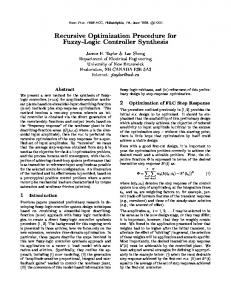
Algorithm 1 The simple unconstrained global optimization algorithm investigated
Bound constrained global optimization problems in the form of
GlobalOptimize ( f , X, ε, Lres , f ∗ ) Y := X; e f := f (m(X)); Lres := {}; Lwork := {}; repeat OptimalComponent(Y, k1 ); Bisection(Y, k1 , U 1 , U 2 ); for i := 1 to 2 do fU := f (U i ); if e f < fU then next i; if f (m(U i )) < e f then e f := f (m(U i )); Lwork := CutOffTest(Lwork , e f ); if w( fU ) < ε then Lres := Lres ∪ (U, fU ); else Lwork := Lwork ∪ (U, fU ); if Lwork , {} then Y := Head(Lwork ); until L = {}; Y := Head(Lres ); f ∗ := [ fY , e f ]; return Lres , f ∗ ;
min f (x) x∈X
are common with X = {xi ∈ [xi , xi ], i = 1, . . . , n}, and xi , xi ∈ R, i = 1, . . . , n. In several cases we can assume that the objective function, f is smooth. Just to name some of the numerous applications of global optimization, we point on some of our recent publications: we solved with such techniques hard mathematical problems arising in the field of qualitative analysis of dynamical systems [2, 5, 6] and discrete geometry, for optimal packing of circles in the square [10, 14]. Global optimization methods have also been applied for theoretical chemical problems [1], and for the evaluation of bounding methods [15]. Matlab is a natural environment for algorithm development and testing. Our aim was to provide an easy to use reliable global optimization method. We have recently completed a similar successful implementation in Matlab for the stochastic GLOBAL procedure [7]. The algorithm investigated now uses only a subroutine calculating the objective function as information on the global optimization problem, i.e. the expression is not required. The procedure does not applies the gradient and the Hessian of the objective function, although these can be computed by the automatic differentiation facility of INTLAB [13]. In other words, we study now that algorithm variant, that does not assume the differentiability of the objective function.
We use only simple bisection along the widest interval component, and no multisection and advanced subdivision direction selection (cf. [9]). The sophisticated techniques based on the p f ∗ heuristic algorithm parameter [3] will be inserted in the future: the present version is planed to be simple and easy to use. The subdivision direction is determined according to the well tested and simple A subdivision direction selection rule (also used in [3]). The algorithm solves also one-dimensional problems. For the Matlab/INTLAB implementation we have followed closely the C-XSC code which was developed for unconstrained global optimization by Mih´aly Csaba Mark´ot based on the algorithm documented in [11]. The
control structures of the two algorithms are identical, while the vectorial array statements of Matlab were applied wherever possible. To use the new method, first install the INTLAB package for interval arithmetic based inclusion functions and verified numerical techniques. Download the compressed archive from the respective web page http://www.ti3.tu-harburg.de/rump/intlab/, and follow the included guide and instructions. The installation requires a few minutes and some level of experience in operating system script programming. Otherwise the hints given in the user guide are sufficient. INTLAB is free for private use and for purely academic purposes provided proper reference is given acknowledging that the software package INTLAB has been developed by Siegfried M. Rump at Hamburg University of Technology, Germany [13]. INTLAB applies a sophisticated rounding that depends closely on the actual hardware. This is why it is easy to implement on a standard PC (also in Linux), while it cannot be used immediately on some modern workstations. When the INTLAB package has been downloaded, decompress the archive, and place the files into a directory, that should be then given as the default directory, where Matlab finds the INTLAB related files. This can be accomplished by setting the Current Directory properly at the top center position of the Matlab window. The next step is to run the script startintlab.m from the main directory: >> startintlab which initiates various global variables and will do much of the rest. In case everything went well, no error message is obtained. Otherwise the user obtains the most important hints how to complete the implementation procedure. Note that you must issue the startinlab command always before using INTLAB, not only the first time. Under Windows, we should change the system variable BLAS VERSION to atlas***.dll choosing ’***’ according to the processor type (for example the full name is ”atlas P4.dll” for a PC with a Pentium 4 processor). The corresponding file is located in the Matlab directory ”...\Matlab\bin\win32\”. If you have the rights of the system administrator, then you can set the BLAS version for all users and threads using the Environment Variables (Control Panel → System Properties → Advanced) dialog box. Otherwise complete the above procedure in the command line window, applying the command set BLAS VERSION="atlas P4.dll" and make sure that Matlab is started then from the same place. Under Linux we can set the new library by the command export BLAS VERSION="atlas P4.so" to reach the above level of readiness. The setting of the BLAS library usually solves all the problems what is reported first by the startintlab procedure.
Table 1: The numerical comparison of the C-XSC and the INTLAB code. Dim stands for the dimension of the problem, NIT for the number of iterations, and NFE for the number of objective function evaluations. Problem S5 S7 S10 THCB BR RB2 RB5 L8 L9 L10 L11 L12 L13 L14 L15 L16 L18 Schw2.1 Schw3.1 Schw2.5 Schw2.14 Schw2.18 Schw3.2 Schw3.7 5 Griew7 R4 R5 R6
Dim 4 4 4 2 2 2 5 3 4 5 8 10 2 3 4 5 7 2 3 2 4 2 3 5 7 2 3 5
C-XSC code NIT NFE 84 307 259 864 310 1,016 5,591 16,779 149 480 75 250 2,339 7,063 21 81 28 109 35 137 141 477 412 1,455 22 81 35 131 52 194 72 270 614 2,100 308 933 32 119 72 232 924 3,011 5,623 17,093 110 355 191 605 216 729 1,547 5,137 355 1,235 1,939 6,695
INTLAB code NIT NFE 83 305 259 864 313 1025 5,591 16,779 149 480 74 247 2,339 7,063 21 81 28 109 35 137 141 477 412 1,455 22 81 35 131 52 194 72 270 614 2,100 308 933 31 117 72 232 924 3,011 5,623 17,093 106 342 191 605 216 729 1,547 5,137 355 1,235 1,939 6,695
The new Matlab/INTLAB based interval global optimization algorithm will also be available soon as a part of the GLOBAL package. The latter is to be downloaded from the www.inf.u-szeged.hu/∼csendes/reg/regform.php web page. The comprised package contains all necessary files, a suitable directory structure and also a testing environment. 3. Computational tests and comparison The numerical comparison aimed to clear whether the new implementation is capable to deliver similar quality results as the old one, and to measure the efficiency in terms of the usual indicators. Hence, we have completed a computational test, and compared the efficiency and the results of the INTLAB implementation to that of a C-XSC, BIAS, and Profil based procedure [11].
Table 2: The numerical comparison of the C-XSC and the INTLAB code. Dim stands for the dimension of the problem, MLL for the maximal list length required, and CPU for the CPU time needed in seconds. Problem S5 S7 S10 THCB BR RB2 RB5 L8 L9 L10 L11 L12 L13 L14 L15 L16 L18 Schw2.1 Schw3.1 Schw2.5 Schw2.14 Schw2.18 Schw3.2 Schw3.7 5 Griew7 R4 R5 R6
dim 4 4 4 2 2 2 5 3 4 5 8 10 2 3 4 5 7 2 3 2 4 2 3 5 7 2 3 5
C-XSC code MLL CPU 14 0.02 43 0.06 58 0.17 1,128 0.36 18 0.00 10 0.00 56 0.33 8 0.00 11 0.00 14 0.00 23 0.10 44 0.71 7 0.00 10 0.00 13 0.00 16 0.01 67 0.35 44 0.00 7 0.00 7 0.00 82 0.06 678 0.48 13 0.00 32 0.01 43 0.07 348 0.11 70 0.03 226 0.48
INTLAB code MLL CPU 13 14.20 43 55.78 55 93.73 1,128 178.58 18 6.64 10 1.72 56 167.84 8 1.94 11 3.41 14 5.22 23 28.23 44 111.63 7 1.45 10 3.09 13 5.69 16 9.55 67 98.92 44 11.63 6 1.89 7 1.44 82 32.19 678 104.73 12 3.80 32 6.59 43 27.44 348 51.39 70 29.44 226 264.31
For the test we used INTLAB version 5.4, Matlab R2007a, and a PC with 1 Gbyte RAM and a 3 GHz Pentium 4 processor. The test problems included all the standard global optimization functions to be minimized, and basically all of those usually applied in comparing interval global optimization methods. Our tables contain results restricted for cases when the INTLAB based algorithm was able to stop within 10 minutes. Otherwise the test problem set is the same as those in other extensive numerical studies, such as [3, 4]. The results are summarized in Tables 1 and 2. The problem names are abbreviated as usual, e.g. S5 stands for Shekel-5, Sch3.2 for Schwefel 3.2, and R4 for Ratz-4 (cf. [3]). The first two columns give the problem names and their dimension. The listed efficiency indicators are the number of iterations necessary (abbreviated as NIT), the number of objective function evaluations (NFE), the maximal length of the working list (MLL), and the required CPU time in seconds (CPU). As compared to the numerical study published in [12],
where the stopping criterion parameter ε was set to 10−8 , now we stopped subdivision when the width of the inclusion function at the actual subinterval was less than 0.01. Our present results are then obviously much weaker than the earlier published, but it is no wonder regarding that in the other case first and second derivative information was utilized as well. Most of the efficiency indicators have the same or very similar values for the two implementations. We discuss here just the larger and systematic differences. The most significant change is definitely in the CPU time needed: the INTLAB based implementation requires on the average ca. 543 times more time to reach basically the same result. The ratios differ from 157 to 981, and the median of them is 523. As a rule, these figures are somewhat smaller than those measured for a more sophisticated algorithm variant based on the inclusion functions of the gradient and the Hessian as well [12]. The highest ratio values are related to cases when the CPU time for the C-XSC version were hardly measurably low. It is also worth mentioning, that the lowest ratios belong to those test problems, that required more computation. The reason for this drop in speed is that Matlab works in interpreter mode, and thus it is no wonder that a machine code program produced by a compiler can reach better times. On the other hand we have to add that we had a well readable, but less optimized coding, and there remained much to improve exploiting the vectorization feature of Matlab. The bottom line of this comparison is that although the easy use of Matlab has its price in speed, still for practical problems the Intlab based interval global optimization method can be a useful modeling tool for early phases of optimization projects. Since the number of iterations, objective function evaluations, and maximal working list lengths are identical for the two algorithms for the majority of test problems, we can certainly conclude that the algorithms are equivalent, and there cannot be significant algorithmic differences. In the remaining cases the slightly changing indicators are caused by the different realizations of the rounding and other hardware depending statements and functions. A smaller part of the CPU time differences is also due to the quicker but less precise interval operations and functions provided by Profil/BIAS. Summarizing our numerical results, we can state that the computational experiences confirm that the new implementation is in several indicators (e.g. number of function evaluations, number of iterations, and memory complexity) in essence equivalent to that of the old one. The CPU time needed is as a rule by at least two order of magnitude higher for the INTLAB version – as it can be anticipated regarding the interpreter nature of Matlab. However, further vectorization coding changes in the algorithm and in the objective functions may improve on that. In spite of the lower speed, the new interval global optimization methods can well be suggested as an early modeling and experimentation tool
for the verified solution of bound constrained global optimization problems.
[12] L. P´al and T. Csendes, “A global optimization algorithm for INTLAB,” Optimization Methods and Software, submitted for publication.
Acknowledgments
[13] S. M. Rump, “INTLAB – Interval Laboratory.” In: T. Csendes (ed.): Developments in Reliable Computing, Kluwer, Dordrecht, pp. 77-104, 1999.
The present work was supported by the grants Aktion ¨ Osterreich-Ungarn 60¨ou6, OTKA T 048377 and T 046822. References [1] J. Balogh, T. Csendes, and R. P. Stateva, “Application of a stochastic method to the solution of the phase stability problem: cubic equations of state,” Fluid Phase Equilibria, vol. 212, pp. 257-267, 2003. [2] B. B´anhelyi, T. Csendes, and B. M. Garay, “Optimization and the Miranda approach in detecting horseshoe-type chaos by computer,” Int. J. Bifurcation and Chaos, vol. 17, pp. 735-747, 2007. [3] T. Csendes, “New subinterval selection criteria for interval global optimization,” J. Global Optimization, vol. 19, pp. 307-327, 2001. [4] T. Csendes, “Numerical experiences with a new generalized subinterval selection criterion for interval global optimization,” Reliable Computing, vol. 9, pp. 109-125, 2003. [5] T. Csendes, B. B´anhelyi, and L. Hatvani, “Towards a computer-assisted proof for chaos in a forced damped pendulum equation,” J. Computational and Applied Mathematics, vol. 199, pp. 378-383, 2007. [6] T. Csendes, B. M. Garay, and B. B´anhelyi, “A verified optimization technique to locate chaotic regions of H´enon systems,” J. of Global Optimization, vol. 35, pp. 145-160, 2006. [7] T. Csendes, L. P´al, J. O. H. Send´ın, and J. R. Banga, “The GLOBAL Optimization Method Revisited,” Accepted for publication in the Optimization Letters. [8] R. Hammer, M. Hocks, U. Kulisch, and D. Ratz, “Numerical Toolbox for Verified Computing I.” SpringerVerlag, Berlin, 1993. [9] R. B. Kearfott, “Rigorous global search: continuous problems,” Kluwer, Dordrecht, 1996. [10] M. Cs. Mark´ot and T. Csendes, “A new verified optimization technique for the ”packing circles in a unit square” problems,” SIAM J. on Optimization, vol. 16, pp. 193-219, 2005. [11] M. C. Mark´ot, J. Fernandez, L. G. Casado, and T. Csendes, “New interval methods for constrained global optimization,” Mathematical Programming, vol. 106, pp. 287-318, 2006.
[14] P. G. Szab´o, M. Cs. Mark´ot, T. Csendes, E. Specht, L. G. Casado, and I. Garc´ıa, “New Approaches to Circle Packing in a Square – With Program Codes,” Springer-Verlag, Berlin, 2007. [15] B. T´oth, J. Fern´andez, and T. Csendes, “Empirical convergence speed of inclusion functions for facility location problems,” J. of Computational and Applied Mathematics, vol. 199, pp. 384-389, 2007.