A Bayesian approach to nonlinear latent variable models ... - CiteSeerX

PSYCHOMETRIKA--VOL.63, NO. 3, 271-300 SEPTEMBER1998

A BAYESIAN APPROACH TO NONLINEAR LATENT VARIABLE MODELS USING THE GIBBS SAMPLER AND THE METROPOLIS-HASTINGS ALGORITHM GERHARD ARMINGER BERGISCHE UNIVERS1TAT WUPPERTAL DEPARTMENT OF ECONOMICS BENGT O. MUTHEN UNIVERSITY OF CALIFORNIA, LOS ANGELES GRADUATE SCHOOL OF EDUCATION ~ INFORMATION STUDIES Nonlinear latent variable models are specified that include quadratic forms and interactions of latent regressor variables as special cases. To estimate the parameters, the models are put in a Bayesian framework with conjugate priors for the parameters. The posterior distributions of the parameters and the latent variables are estimated using Markov chain Monte Carlo methods such as the Gibbs sampler and the Metropolis-Hastings algorithm. The proposed estimation methods are illustrated by two simulation studies and by the estimation of a non-linear model for the dependence of performance on task complexity and goal specificity using empirical data. Key words: Gibbs Sampler, LISREL model, Metropolis-Hastings algorithm, Non-linear functions of latent regressors.

1.

Introduction

R e s e a r c h scientists in p s y c h o m e t r i c s , e d u c a t i o n a n d m a r k e t i n g o f t e n w o u l d like to c o n s i d e r m o d e l s w h i c h c o n t a i n q u a d r a t i c a n d / o r i n t e r a c t i o n t e r m s in t h e l a t e n t v a r i a b l e s . A typical p r o b l e m is t h e e s t i m a t i o n o f t h e s i m p l e q u a d r a t i c m o d e l Y = 3'0 + 3'1~ + 3'2~2 -{- if,

(1)

w h e r e ff - 0g(0, 4') is a d i s t u r b a n c e t e r m w h i c h is u n c o r r e l a t e d w i t h t h e u n o b s e r v e d r a n d o m v a r i a b l e ~ - N ( 0 , 1). ~ is a l a t e n t variable. 3'o, 3'1 a n d 3'2 a r e r e g r e s s i o n coefficients a n d y is a r a n d o m v a r i a b l e t h a t is c o n d i t i o n a l l y n o r m a l g i v e n {~with y - 0g(3'0 + 3'1~ + 3'2~2, 4'). H o w e v e r , y is u n c o n d i t i o n a l l y n o t n o r m a l , b u t follows a d i s t r i b u t i o n w h i c h is a c o n v o l u t i o n o f a s t a n d a r d n o r m a l a n d a X12 variable. T h e m e a s u r e m e n t m o d e l for ~ is g i v e n as a f a c t o r a n a l y t i c m o d e l with

x=v+A~+6,

(2)

The first author is indebted to the Graduate School of Education and Information Studies at UCLA for providing a visiting professorship during the winter quarter 1994. The work of the first author was supported by a grant from the Deutsche Forschungsgemeinschaft. The work of the second author was supported by grant 1K02AA00230-01 from NIAAA and by grant 40859 from NIMH to C. Hendricks Brown's Prevention Science Methodology Group. The authors thank Donald Rubin and C. Hendricks Brown for a critical reading of the first draft of the paper. They are especially grateful for the technical assistance of J6rg Wittenberg of the Bergische Universitfit Wuppertal who designed the program BALAM (Bayesian Analysis of Latent Variable Models). The data for the empirical example have been generously provided by Heinz Holling of the University of MOnster, Germany. The authors are indebted to an associate editor and to three anonymous reviewers of Psychometrika whose criticisms, comments and suggestions have been very helpful. Requests for reprints should be sent to Gerhard Arminger, Department of Economics, FB6, Bergische Universit~t--GH Wuppertal, D-42097 Wuppertal, GERMANY. 0033-3123/98/0900-95442500.75/0 © 1998 The Psychometric Society

271

272

PSYCHOMETRIKA

where x - r × 1 is a vector of observed variables, 8 - r X 1 is a vector of measurement errors that are uncorrelated with {~. v is a r × 1 vector of regression constants and A is a r × 1 vector of factor loadings. As in classical factor analysis (see for instance Lawley & Maxwell, 1971) it is assumed that the errors are normal and uncorrelated, that is 8 - 3~(0, 19) with 19 = diag {'011. . . . . Orr}. The model (1) and (2) may be extended to a random vector ~ = (~1, ~2, - - - , ~,~)' allowing to deal with quadrat!c or higher order polynomial terms, ~2, ~3 and/or interaction of the form ~1~2, ~1~3 and so forth. It is assumed that the ~ × 1 vector ~ follows a multivariate normal distribution N(0, q~). Until now, estimation of the parameters y, q~, tO, v, A, O has been carried out (Hayduk, 1987; Kenny & Judd, 1984) in the context of L I S R E L models by writing the observed variables in the model of (1) and (2) asxj = vj + hj~ + ~i,J = 1 . . . . . r and then including the variables xf = (vj + hj~j + 6j) 2 as additional indicators for ~2 in the measurement model. Then, a LISREL model with ~ and ~2 as latent regressor variables is estimated. This solution is often not optimal in the following ways: •

•

•

•

Under the assumption that if, ~ and 6j, j = 1 . . . . , r are normally distributed, the joint distribution of (y, x l . . . . , Xp, x 2 . . . , XZp) is not multivariate normal. ML estimation based on the normal distribution of (y, xl . . . . . xp, x 2 . . . . x 2) therefore yields consistent estimators for the parameters (% ~ , tO, v, A, O) collected in a vector O but not for the asymptotic covariance matrix of the ML estimator bgL. To our knowledge, the natural remedy of Pseudo ML estimation (Arminger & Schoenberg, 1989) has not been applied to this model to deal with non-normality. However, weighted least squares (WLS) estimation (Browne, 1984) has recently been applied to this model by J6reskog and Yang (1996). These authors therefore obtain consistent estimates of the chi-square statistic for model fit and the standard errors of the estimated parameters. Computing parameter estimates with the LISREL program (J6reskog & S6rbom 1993; J6reskog & Yang 1996) or equivalent programs such as LISCOMP (Muth6n, 1988) and MECOSA 3 (Arminger, Wittenberg & Schepers, 1996) is rather cumbersome. Although one of the main obstacles, namely the inclusion of all possible cross products of observed variables as indicators for a latent interaction model, has been removed by J6reskog and Yang by showing that the inclusion of one product variable is sufficient for identification, it is still rather tedious to write the nonlinear equations for the covariances of cross products as a function of the model parameters. Good examples are found again in J6reskog and Yang. The ML and WLS estimation techniques draw on large sample theory and may not be suitable for small or medium sample sizes. An additional problem is here the number of variables. If the number of observed variables is already large, this number is further increased by the addition of squares and cross products of observed variables. The nonlinear models using squares and interactions of latent variables may not be general enough to specify more complicated substantive models. Therefore it should be possible to specify general nonlinear models as in nonlinear regression analysis.

We propose to deal with the problems of nonnormality and a general specification of nonlinear latent variable models as well as with the problem of small sample sizes by using a Bayesian approach to formulate the model and Markov Chain Monte Carlo (MCMC) methods such as the Gibbs sampler (Gelfand and Smith 1990, Tanner 1993) and the Metropolis-Hastings (M-H) algorithm (Chib & Greenberg, 1995; Hastings, 1970; Metropolis, Rosenbluth, Rosenbluth, Teller, & Teller, 1953; Tanner, 1993) to estimate the posterior distributions of the parameters given the data.

GERHARD ARMINGER AND BENGT O. MUTHt~N

2.

273

The Nonlinear Latent Variable Model

We introduce a nonlinear version of the L I S R E L model (J6reskog & S6rbom, 1993). Let ~i be a fit × 1 vector of random variables that is multivariate normal with ~i ~ 0g(0, • ). Let ai = g(~i) a m x 1 deterministic function of ~i that is known. A p x 1 random variable vector 71i is connected with oei through a linear regression model (3)

~ i = ~I0 "~ l~oli ~- ~i,

where the p × 1 random variable ~,/~ ~N~(0,~ ) is a disturbance, 3'o ~ P × 1 is a vector of regression constants and F ~ p × m is a matrix of regression coefficients of ~li on ai. It should be noted that the model is linear in the parameters, but is nonlinear in the components of ~iThe random variables ~i and ~li are connected to observed variables xi ~ r × 1 and 3', ~ s × 1 with the usual factor analytic measurement models x; = v~ + A x ~ + a~, a, ~ ~'(0, Oa),

(4)

y~ = Vy + Ay'lqi + I~i, e i ~ , ~ ( 0 , O e ) .

(5)

For simplicity, it is assumed that O8 and O~ are diagonal matrices according to the classical factor analytic tradition (Lawley & Maxwell, 1971). The nonlinear latent variable model defined in (3) through (5) is abbreviated as the A-M model. This model includes some important special cases. The first special case is a polynomial regression model in the latent variable ¢i for a univariate dependent variable Yi a i = (¢i' ¢2. . . . .

(6)

Cp) t

ni = 3"0 + F a i + ~ , ~ ~ X ( O ,

~),

(7)

x, = v~ + A x ¢ , + ~,, ~ ~ ~ ( 0 , O~),

(8)

Yi = ?Oi"

(9)

T h e u s u a l l i n e a r m o d e l T/i = 3'0 -Jr 3'1~i "q- ~i is replaced by a polynomial m o d e l ~i = 3'0 + 3"]~i + . . . 3"p~ + ¢i. This model allows formulation of a regression model that is non-

linear in the variables and has errors in the variables. It may also be considered as a partially linear and partially nonlinear factor analytic model where Yi is an indicator variable that is nonlinearly dependent on the factor score ~i. The second case is a model with a generalized second order polynomial of the vector ~i and a univariate dependent variable Yi (lO) n~ = 3'o + Fa~ + ~, ~i ~ :¢(0, q,),

(11)

xi = Vx + Ax(~ + & , ~ ~ ~0(0, Oa),

(12)

Yi = ~i.

(13)

This model allows for first order interactions of latent variables ¢ij, J = 1 . . . . . ~ in the regression model for Yi. Of course, higher order interactions may be formulated in the same way. Again, this model may be also thought of as a nonlinear errors in the variables model and as a partially linear and partially nonlinear factor analytic model. Finally we consider ~i as a p-th order generalized polynomial and formulate a polynomial factor analytic model:

274

PSYCHOMETRIKA. Cl~i = PP(~il .....

~ir~) = (~il,

• • • , ~ir~, ~21, • • • , (~i(rTt-p+l) ~i :

ai'

....

~ir~))',

(14) (15)

yi = vy + Ayrl/+ el.

(16)

It is important to note that the A-M model may be overparameterized for certain applications. For instance, if the measurement model for Yi = Vy + Ay~li + Ei contains regression constants that are estimated from the data, ~/0 may not be identified as seen from the expected value of the reduced form of Yi given ~i: E(yil~/) = vy + Aye'0 +

Ayrg(gi).

(17)

In this case, Y0 must be set to a fixed value such as Y0 = 0. Additional identification restrictions may be necessary for specific models. As one of the anonymous reviewers has pointed out, the choice of g(~) is not completely arbitrary. Restrictions have to be imposed to ensure a proper posterior for ~1 and g. Examples of a bad choice of g(g) are g(g) = 0 which eliminates the data x or to choose a = g(~) so that the components of ot are linearly dependent. In this case, the posterior distribution would collapse in dimensionality. The issue of proper posteriors is discussed in subsection 3.3. 3.

The Bayesian Framework

The usual way to estimate the parameters in the vector O = vec {Y0, F, ~ , ap, Vx ' Ax' 0 8 , Vy, Ay, O~} has been a frequentist approach. Given the normal distribution of ~i, gi, 6i and ei, the parameter vector O has been estimated with ML method. This approach works nicely if the function g in ai = g(~i) is the identity function. However, if g is a nonlinear function, such as a polynomial, the unconditional distribution of rli, and therefore of Yi, is not normal. To avoid these complications we switch from the frequentist to the Bayesian viewpoint and consider only the data {yi, xi}, i = 1 . . . . , n as fixed and--in addition to the random variables ~i, gi, 6 / a n d e/--the parameter vector O as a random variable. A Bayesian framework has been used before in the context of linear factor analysis by a number of authors, for instance by Lee (1991) who considered the posterior distribution of the matrix of factor loadings, the covariance matrix of factors and the covariance matrix of errors and Press and Shigemasu (1989) who considered additionally the posterior distribution of factor scores. Our aim is to estimate the joint and marginal distribution of ~, ~1, and O given x and y. We are interested in the posterior density of ~, rl, and O given the data x, y. For conditional density functions we use the formulation of Gelfand and Smith (1990), where [ylx] denotes the conditional density of a random vector Y at the value of y conditional on a fixed value x. The joint posterior is therefore denoted by [~, rl, Olx, y]. 3.1

Prior Distributions

As noted before, the random variables gi, gi, 6 / a n d e i are multivariate normal with and e i ~ .g(O, 0 ~ ) . ~i, ~i, 6i, and e i are assumed to be independent of each other. O 8 and Oe are assumed to be diagonal. The components {~0, F}, @, aI~, {Vx, Ax} , 08, {vy, Ay}, Oe of O are assumed to be stochastically independent. The priors for the components of O are chosen as conjugate priors and given in detail below. We define the p ( m + 1) dimensional column vector ~, as the vectorized form of ~/0 and F, that is ~i ~ .]~(0, (I)), ~i ~ .N'(0, lll), ~i ~ .]~'(0, 08)

GERHARD

~t =

(701,

')tll ....

ARMINGER

, Ylrn,

AND

Y02,

BENGT

275

O. MUTHI~N

"Y21, • • • , Y Z m ,

• • • ,

")lpm) t"

(18)

In a similar way, we define ~x,k = ( Vx,k, Xx,k,1 ....

, l~x,k,Fn)t,

(19)

~y,j : (1)y,j a t~y,j,la .'.

, Ay,j,p)t.

(20)

and

as the vectorized forms of the constant and factor loading coefficients for the k-th component of x and thej-th component of y. These vectors are assumed to be independent and to follow the conjugate priors ~/~ N(y*, nv),

(21)

Ax,~~ N(X*,k, n x , ) ,

(22)

~y,j ~ ~(Xy, j, ~-~y,j)a

(23)

where the expected values y*, A* k, A,*,j and the covariance matrices l~v, ~x e, ~y,j or respectively the precision matrices' 1 ~ i 1~, 1, ~£1 are chosen by the researcher. Before we turn to the conjugate priors of the covariance matrices ~ and @, we review briefly the Wishart and the inverse Wishart distribution. The following definition of the Wishart distribution is used. The p × p-dimensional positive definite matrix A follows a Wishart distribution with p × p-dimensional positive definite parameter matrix B and d degrees of freedom if the density is given by A - W(B, d) ~

Igl-d/21Al - -'/2

exp

- ~ tr (B-~A)

(24)

where d -> p (see Anderson, 1984, p. 249; and Carlin & Louis, 1996, p. 168). We note that E(A) = d B . The inverse matrix A* = A -1 with parameter matrix B* = B -1 has the density A* ~ W-I(B *, d)

~

IB*Id/2IA*I -(d+p+l)/2 exp - ~ tr (B*(A*) -1)

(25)

as shown by Anderson (1984, p 268). B* is called the precision matrix. Following Anderson (1984, p. 269) further, his corollary 7.7.1 says: With an inverse Wishart prior for the covariance matrix X, 2~ ~ W-l(dl'~, d)

(26)

where (dl-l) is a precision matrix and A = nS - W'(2£, n)

(27)

×IS - ~V-l(nS + d ~ , n + d).

(28)

we find the posterior

The notation of Anderson (1984) is changed slightly in the sense that (dl~) is the precision matrix of the inverse Wishart distribution. Hence, a weak prior for X has a low d and a small matrix ~ so that nS dominates in the posterior form nS + d ~ . S is the sample covariance matrix computed from n data points centered about the expected value. The conjugate prior for the covariance matrix ~ of the random vector ~ - N(0, ~ ) is given in terms of the inverse Wishart distribution

276

PSYCHOMETRIKA q* -- W - l ( d . ~ . ,

d.)

(29)

The parameter matrix l-l,I, and the degrees of freedom d,i, in (29) are chosen by the researcher. Similarly, the conjugate prior for the covariance matrix • of ~ - 0g(0, @) is given by

-- W - a ( d , l l , , d . ) .

(30)

Since the covariance matrices 0 8 and O~ are diagonal, we can use the conjugate priors for the variances of the error terms in the measurement equations. The prior is given by the inverse Gamma distribution for a random variable s with s > 0

s - ,,~(a, b) = F(a)-lbas-(a+l) exp ( - b) where a (a > 0) is a shape and b (b > 0) is a scale parameter & Rubin, 1995, p. 474). The expected value ofs is E(s) = b/(a chi-square distribution is a special case of the inverse gamma b = 1/2 where df is the number of degrees of freedom. The ®,,kk then follow inverse Gamma distributions ~)6,jj ~

~(as,jj ,

(31)

(see Gelman, Carlin, Stern, - 1) for a > 1. The inverse distribution with a = df/2, random variables ®8,jj and

b~,jj)

(32)

Taken together, this implies that the posterior distribution [O, ~, rlly, x] is a proper posterior distribution. ~ e,jj ~

,.~C~( a ~,jj, b ~,jj)

(33)

where a~,jj, ba,jj and a~,jj, b~,jj are chosen by the researcher. Several of the conditional distributions used in this paper for Gibbs sampling can be derived using known Bayesian results for the two linear models discussed in subsection 3.3.

3.2 Posterior and Likelihood It is clarifying to express the joint posterior distribution in terms of the densities of all the distributions and write out the likelihood as the product of marginal and conditional distributions. The issue of whether proper priors lead to a proper posterior distribution can then be also considered. Let the parameters of the model be denoted O and let [z] denote a density for the random variable z. Using the assumptions of the A-M model, we note that [~llx, ~, O] = [~1[~, O] and [y[rl, x, ~, O] = [Y]~I, O]. Denoting the observed data distribution [y, x] as c, the posterior distribution [O, ~, ~IIY,x] for the unknown parameters and the latent variables conditional on the observed data may be expressed as c x [O, ~, nlY, x] = [O][~lO][xl~, O][nl~, O][yln, O]

(34)

where [O] is the prior for the parameters. Here, the conditional distributions [~lO], [xl~, O], [~[~, O], and [yl'rI, O] are all multivariate normal according to the A-M model. The likelihood L is L

(f

= [y, xL< : j j [elo][xle,

o][yi,,, o] d,,

In (34), a proper posterior distribution is obtained if the following integral converges

277

GERHARD ARMINGER AND BENGT O. MUTHEN

f

c = [y, x] = J L × [O] dO.

(36)

With g(~) = [, [[, rl] and [y, x] are multivariate normal. In this case, it is well-known from Bayesian analysis using conjugate priors that this gives a proper posterior for 19, see for example, Gelman, Carlin, Stern and Rubin (1995, pp. 80-81). The propriety of the posterior for other choices g(~) v~ ~ needs to be investigated separately for each class of g(g). 3.3

Posteriors for Covariance Matrices and Regression Coeyficients

3.3.1

Random Case

We consider a linear model for the p-dimensional vector vi for observation i(i = 1, 2 . . . . , n) with known p × r matrix A, r-dimensional random coefficient vector Ki, and p-dimensional residual vector ei, Vi = A K i + el,

(37)

K i ~ ~'(1~0, ~ ) ,

(38)

for which it is assumed that

where ]£ is an r × r covariance matrix. We further assume that the residuals eij are unco~-elated and have variances V(eo) = o'2; j = 1 . . . . .

p.

(39)

The following proper prior distributions are assumed t% ~ 3 ( ( e , D ) ,

(40)

-- neV-l(dIl, d),

(41) (42)

o'] ~ 8 ~ ( e , f ) .

Here, a vague prior for •0 is obtained by choosing D-1 = 0. As seen below, this results in the prior mean c vanishing from the posterior. As in section 3.1, ( d ~ ) is the precision matrix for the inverse Wishart prior of 1~. A low value of d relative to n gives a vague covariance matrix prior; the smallest admissible value is r, the number of rows in £. A vague prior for o.~ is obtained by choosing e close to zero and f large. Well-known results (see, e.g., Anderson, 1984, p. 269; Carlin & Louis, 1996, pp. 168-169; and Lindley & Smith, 1972) give the conditiona~osterior distribution for K0 conditional on Vl, V2 . . . . , Vn, R1, R E , . . . , Kn, 0~1, 0"2. . . . . Up, K0 - 3¢(V(n~-lk + D-le), V), for £ given Vl, v 2 , . . . , vn, ~¢1, •2 . . . . . ~¢n, ~'0, o.2, 0222. . . . .

(43)

O~p,

~ %r-l(nS + d l ) , n + d), and for o,2 given vl, v2. . . . , vn, K1, •2 . . . . , •n, K0, °~1, o~ . . . . . o.2 ~ # ~

+ e,

o~p, £ - 1

2 ~ (vi - AIci)'(v, .... AKi) + f - 1 i=1

Here,

(44)

.

(45)

278

PSYCHOMETRIKA V :

( n X -1 +

k = -

D-l) -1,

(46)

Ki,

(47)

t:/ i=1

nS = ~ ( K / - ~¢0)(K/- K0)'.

(48)

i=1

While the above posterior distributions are conditional on the other unknowns, it is well-known that the joint posterior distribution is also proper (see Gelman et al. 1995, pp. 80-81). Hobert and Casella (in press) further discusses properties of posteriors with various variance priors for the mixed linear model and show conditions under which proper posteriors are obtained even with "power" improper priors on the variance parameters. 3.3.2

Fixed Case

We consider the q-dimensional vector vi for observations Vl, v2, . . . , vn, the known q × r matrix Ai, the r-dimensional parameter vector •, and the q-dimensional residual vector ei, vi = AiK + ei,

(49)

where V(ei) = X, a q × q covariance matrix which is assumed known. We assume the proper prior distribution K - ~(K0, 1~),

(50)

where ~0 and 1"1 are known. Using well-known results (see, e.g., Carlin & Louis, 1996, p. 41; Lindley & Smith, 1972), we find that the posterior distribution for K conditional on Vl, V2, . . . , Vn is -- W ( O d , D)

(51)

where =

Ai~

Ai

+

l-1-1, and

(52)

i=1

A weak, proper prior is obtained by choosing the precision matrix 1~-1 close to a zero matrix. 4.

The Components of Markov Chain Monte Carlo Sampling

To describe the joint and marginal posterior distributions of ~, ~ and O given x and y we use the Gibbs sampler (Gelfand & Smith 1990; Geman & Geman, 1984), the M-H algorithm (Chib & Greenberg, 1995; Hastings 1970; Metropolis et al., 1993; Tanner, 1993) and a combination of both (Mtiller 1994). Easily accessible descriptions of the Gibbs sampler are found in Arnold (1993) and Casella and George (1992). Statistical theory underlying Markov Chain Monte Carlo (MCMC) methods such as the Gibbs sampler and

279

GERHARD ARMINGER AND BENGT O. MUTHEN

the M-H algorithm is found in Chib and Greenberg and Tierney (1994). General references on Bayesian computations are Besag, Green, Higdon and Mengersen (1995) and Gilks, Richardson and Spiegelhalter (1996). The relationship between iterative simulation techniques and the more familiar EM algorithm is discussed in Rubin (1991). In the Gibbs sampler one samples iteratively from the conditional distributions [~(k+,), rl(k+l)lX' y, O(k)],

(54)

where k + 1 denotes the present iteration and the distributions [O~qk+,)tx' y, ~(*), ~)(k), 0 (k+'>lq-I,'q(k) I

(55)

where O(qk+ 1) is the q-th subvector of the vector 0 at the present iteration. After a burn in phase, the conditional distributions converge to the posterior distributions of the parameters of interest. We start by assuming that ~i and rli are known for the k-th iteration taking on the values ~k), rl~k). Then we can compute or!k) = g(~jk)).

(56)

4.1 Parameters of the Regression Model The conditional distribution of the regression parameters in the model (3)-(5) is [3"0, rlx, y,

)), 0 - (v0, r}].

(57)

Here, t9 - {3'0, F} is the set of all parameters in O without the set of parameter that are elements of 3'0 or F. Since the prior distribution of 3' from (18) is multivariate normal with 3" - N'(3"*, llv) where 3"* is the known a priori expected value and II v is the known a priori covariance matrix of % the posterior distribution of 3" given ~i and (~i may be derived using the results of subsection 3.2.2. The values ai are written in a regressor matrix Ai - p x (p(m + 1)) defined by A, = Ie×, ® (1, or,),

(58)

where ® denotes the Kronecker product. With this notation ))i = &3" + ~i

(59)

where rti , Ai and V(~) = ~ are known in the k-th step of the Gibbs sampler. Application of (51) and substituting rti for vi, 3' for re, and W for I~ yields that the posterior distribution of 3" is multivariate normal with expected value. E(T) =

A ~' -' &

+ ll~ q

i=1

A~aIt-Jn-~ i=1

and covariance matrix V(3") =

A~W-'A~

+ ~"~-1

)'

.

] ) + fl-~7 *

(60)

(61)

i=l

Hence 3"(k+1) is drawn from the posterior distribution ./~'(E(3"), V(3")) where ai, ~i and W are replaced by a~(k), r)~k) and W (k). A weak proper prior is obtained by choosing the precision matrix ll~ 1 = 0. Then, the equations (60) and (61) simplify to

280

PSYCHOMETRIKA

E(T) =

A~-IAi

Ai~

i=1

lfli ,

(62)

i=1

and

V('y) =

i=1 ~

A~r-IAi)-I"

(63)

Alternatively, one might set 3,* to correspond to the expectations of the researcher, for instance as a vector of zeros and set g ~ l to a diagonal matrix with small values, for instance 0.01. The conditional distribution of [~lx, y, ~, rl, O - {~}]

(64)

is found using the inverse Wishart distribution. Since ~ ~ ~ × 1 is multivariate normal with J¢(0, ~ ) and • follows the inverse Wishart prior ~h/'-l(d~l~, d~), the posterior covariance matrix ~(k+l) follows an inverse Wishart distribution with parameter matrix

i=1~ ~(k)~(k)t+ d,~.)

B. =

(65)

and n + d~ degrees of freedom using equations (44) and (48) and substituting ~i for Ki, 0 for to,0,d~ for d and ~ for 1~. A weak, proper prior for • is obtained by choosing d~ small relative to n, say d~ = ~ and setting ~4, to a diagonal matrix with small positive values. The conditional distribution of [~I~lx, y, ~, #, 0 - {W}]

(66)

is also found using the inverse Wishart distribution. Since ~ ~ ~o × 1 is multivariate normal with J¢(O, ~ ) and ~ follows the inverse Wishart prior ~¢¢-i,( d ~ , ~ , d~), the poste rl"or covariance matrix ~(k+ 1) follows an inverse Wishart distribution with parameter matrix

---~

--

"'i

r

)\,|i

"

i=1

-~

d,fl. ,

(67)

and n + d,t, degrees of freedom using (44) and (48) and substituting ~]i -- A i ~ for •i, d,I, for d and I-Lt, for ft. A weak, proper prior for W is obtained by choosing d,t, small relative to n, say d~ = p and setting 1~,~ to a diagonal matrix with small positive values. If # is univariate, then ~ - ~'(0, ~ ) and • is assumed to follow an inverse gamma distribution ~ ( e , f ) as prior. From equations (42) and (45) we find that • has the posterior distribution ~ ( a , b) with parameters n

a = ~- + e

(68)

n b = ~ ~] i=1 (~}k) _ A}k)y(k))2+ f-l.

(69)

and

GERHARD ARMINGER AND BENGT O, MUTHEN

281

If e is chosen as an integer × 1/2, for instance e = 1/2, then the variance qAk+0 can be sampled from an inverse X2 distribution with n + 2e degrees of freedom, f - I is set to a small value, for instance 0.01. 4.2

Parameters o f the Factor Analytic Models

Given r/i and the fact that O~ is diagonal, one finds the posterior distribution of the vector Xy,j = (vy,/, Ay,j,1. . . . , Ayd,p)' for t h e j t h component of Yi from the factor analytic regression equation y~j = vy,j + Ay,j,19Qi 1 -4- ...

+ Ay,j,p~i p .4- eij

(70)

and the prior for Xy,j ~ Ar(X~,j, fry,j). Application of (51) and substituting Xy,j for re, O~,1. for X -1 and aqj for Ai andylj . . . . , Ynj for Vl . . . . . vn shows that the conditional distribution

[L-, Aylx, Y, g,

~!, O - {vy, Ay}]

(71)

is found by drawing each vector Xy,j from a p + 1 dimensional normal distribution with expected value I x , yj + l~yjAyj) -1~* + l~y.)) - 1 ,~' O -~,yy

E(Ayd) = ( ® ~ Z ' Z

(72)

and covariance matrix (O~,~Z'Z + fry-1d) -1 .

(z!)

(73)

The n × (p + 1) regressor matrix Z is defined as

Z =

with

zi =

(1, nil . . . . .

nip)"

(74)

The regressand vector yj = (Ylj, Y2j . . . . . Y~j)'. A weak proper prior is obtained by setting the precision matrix 11~,/ = 0. Alternatively, one might choose X~) to reflect the expectation of the researcher, for instance as a vector of ones and set Dg~~ to a diagonal matrix with small values, for instance 0.01. The conditional distribution [O,Ix, y, ~, ~!, 0 - {O~}]

(75)

is found by considering that O. is a diagonal matrix and each element O~,jj follows an inverse Gamma distribution (cf. equation (33)) Oe,jj ~ #~(ae,ij, b~,yj). From (42) and (45) we find that O~,jy has the posterior distribution 3~q3(a, b) with parameters n

a = ~- + a~dj

(76)

b = -~ ~. (Yij - Vy,j - Ay,j~i) 2 + b~.~

(77)

and n

i=1

where A ~ is thej-th row of A,. To compute o(~k.+1) in the Gibbs" sampler, v,, i, A,, ~and r/i are replaced by v(~), A~(k,) and~r/! k). If a ~ , is chosen as an integer × 1/2, for"insta'nce a ~ , = 1/2, then the variance O(~g,y~1) can be sampled from an inverse X z distribution with n 2a~,yj degrees of freedom, b ~ . is set to a small value, for instance 0.01.

282

PSYCHOMETRIKA

Given gi and the fact that O~ is diagonal, similar calculations can be made to find the marginal posterior distributions of ( v x, Ax) and O 8. Since Ax, k - -- (Vx, k, Ax,~l, . . . , ;tx,k,,~ ) follows the prior N(A*,k, llx,k), (51) may be applied again by substituting Ax,k for J¢, ®~,~k for X -1, gk for A/and x l k . . . . , Xnk for Vl. . . . . vn. Then the conditional distribution [vx, A~lx, y, ~, *1, O - {v~, A~}]

(78)

is found by drawing each vector Ax,k from a (fit + 1) dimensional normal distribution with expected value E(AxS) = ( O ~ k U ' U + l-l~j,) -1 -1 (O~,kkU -1 , Xk + l-l~j¢A~,k) -1 *

(79)

and covariance matrix v(Xx, ) : (o

,Lu'u +

-1

-1

.

(80)

~ir~)-

(81)

The n x (rh + 1) regressor matrix U is defined as

U =

with ui = (1, ~il . . . . . n

The regressand vector Xk = (Xl/¢, X2k. . . . . Xnk)'. Sometimes, special identification restrictions have to be taken into consideration. For instance, if only a single factor ~ ~ 3V(0, ~ ) is assumed with measurement model x i = Vx + Ax~i + 6i with 6/ ~ N(0, O,) and error variances greater than 0, then • is only identified, if Ax is restricted, for instance by setting A~,11 = 1, so that the equation Nil = llx,l + ~i "~- ~il

(82)

holds. Since Ax,H need not be estimated, the parameter vector AxA consists only of the element Vx, 1. The n × 1 regressor matrix U in (81) consists of a vector of ones. The regressand vector is given by xk = ( X l k -- ~1, . . . , Xnk -- ~ n ) " The conditional distribution [O~lx, y, ~, rl, 0 - {O~}]

(83)

is found by considering that 0 8 is a diagonal matrix where each element Oa,kk follows an inverse Gamma distribution. (see (32)) Oa,kk -- .~N(aa,kk, ba,kk ). From (42) and (45) we find that Oaj~k has the posterior distribution #~3(a, b) with parameters n

a = ~ + a~Sk

(84)

and (xik -- vx.k -- Ax.k~i) 2 + b~-~k,

b = -~

(85)

i=1

where A x k is the k-th row A x. To compute o~k.~ 1) in the Gibbs sampler, v x k, A x k and are replaced by Vx(.k~,A(k~ and ~k). If aa,kk is chosen as an integer ×1/2, for instance a a k k = 1/2, then the variance o~k,~1) can be sampled from an inverse X2 distribution with n '+ 2aa,kk degrees of freedom, b ~ l k is set to a small value, for instance 0.01.

283

GERHARD ARMINGERAND BENGT O. MUTHEN

4.3 Drawing from the Distribution of Latent Variables The conditional distribution of ~ and ~1 given x, y and O is now considered. Since independence of (xi, yi) and ~i, rli, i = 1 . . . . . n across units has been assumed, it suffices to look at the conditional distribution [~i, ~/i[x,, y,, O].

(86)

Unlike for the conditional distributions considered before, we have not been able to derive a form of the conditional distribution from which values of (~i, ~i) given xi, Yi, O can be sampled easily. Therefore, we use the Metropolis-Hastings algorithm as described in Tanner (1993), and Chib and Greenberg (1995) to generate values of (~i, rli) that follow the conditional distribution of (86). Let (~0), ~q(0)) be the current value and (~(1) ~(1)) denote the value generated by a distribution from which one can easily sample. This easilX sampled distribution is called the driver (driving or proposal distribution). Let ~r(°) and zr(1) denote the density of (86) evaluated at (~(0), ~(0)) and (~0) ~0)). Then the value c = min

( ~r°> } ~rg~, 1

(87)

is calculated. If c = 1, then the value (~(1), ~1(1))is accepted and becomes the current value. If c < 1, then the value (~(1), ~1(1)) is accepted only with probability c, otherwise (~(0), .11(0)) stays the current value. This algorithm ensures that the accepted values form a sample from the distribution of (86). To use the M-H algorithm we have to compute 7r(°) and 7r(1) and to sample from a simple driving distribution. First, we deal with the computation of ~.(0) and 7r0). We note that [~i, ~iIXi, Yi, O] may be written as [~i, rlilx/, y~, O] oc [~i, #,lO][x,l~i, ~i, O][y,]x~, ~i, ~li, O] =

n, lO][x,l

i,

O][y~]~li, O].

(88)

The last equality holds because xi depends only on ~i and not on ~li and because Yi given rli does not depend on ~i or xi. Substituting [~,, nil O] = [~,lO][n,l~,, O]

(89)

[~i, rl,]xi, Yi, O]~[~[O][rlit~i, O][xit~i, O][Y~lrli, O].

(90)

yields the expression:

Since the ratio rr(1)/~"(°) does not depend on the proportionality constant, it suffices to evaluate [gi)o][nilgi, O][xi[~i, O][y~lne, ,9] at the points (~(0), rl(0)) and (~(1), rl(1)). The components of this joint density of ~i, ~i, xi and Yi given O are implied by the model in (3) through (5). An important special case occurs if y = rl, that is, the measurement model for y is given by y = rb In this case, we consider the conditional distribution: [~ilx~, Yi, o]~[~,tO][x,l~, O][y~lgl, o].

(91)

For the proposal distribution, we take the joint distribution [~i, ~ilO] = [ ilo][nil i, o] by first sampling ~ from the a priori distribution X(0, ~ ) and then sampling )1 from X(~/0 + Fa(~), ap) where ~ , 3'0, F, and xI~ are evaluated at the kth iteration step. Alternatively, we sample ~ from the conditional distribution [~]x, O] which may be derived from the joint normal distribution of x and ~.

284

PSYCHOMETRIKA

Hence, the conditional distribution of ~ given xi is multivariate normal with E(~lx, vx, O, Ax, O~) = ~A~'(Ax~A" + O~)-l(xi - u~)

(93)

and covariance matrix V(~lxi, v~, 4 , A~, 08) = @ - ~ A ~ ( A ~ A " + O~)-lAxO = ( 0 -1 + A~O~IA~) -1.

(94)

Since the proposal distribution does not depend on (~(o), ~1(0)), the M-H chain generated in this way is called an independence chain (Tierney, 1994). 5.

Analysis of Simulated Data

The Bayesian analysis described above is investigated using two simulated data sets, the first coming from a model with one latent regressor variable and its quadratic term, the second coming from a model with two latent regressor variables and an interaction term between the two regressor variables. The sample sizes used are in both cases n = 100, n = 250 and n = 500. A total of 100 Monte Carlo replications were used to study the variation across different generated samples. Important questions for the practical implementation of Gibbs sampling are whether to use multiple runs with different start values or to use a single run, whether to use--after a burn in phase--each value of the Gibbs sampler or to use a subsample and how to judge convergence of the Gibbs sampler. Each of these questions has been debated in the literature. Following Chib and Greenberg (1996), we have implemented the single run method because it is less wasteful in the number of iterations needed. Following the arguments of McEachern and Berliner (1994) we use the full Gibbs sample rather than subsampling because subsampling is inefficient in comparison to full sampling. Methods of judging convergence from multiple runs are found in Gelman and Rubin (1992) and from a single run in Ritter and Tanner (1992). Given the massive amount of computing for analyzing the Monte Carlo replications and that the number of iterations for each analysis should be comparable we have settled for a burn in phase of 500 Gibbs cycles and additional 2000 Gibbs cycles from which parameters of the posterior distribution are estimated. The number of M-H cycles is critical. We started with 5 cycles yielding unsatisfactory results while 20 cycles gave satisfactory results in all simulations performed. The check, how many cycles are necessary, can only be done by varying the numbers of cycles systematically and checking for convergence of results. In the simulation, the convergence to the true values suffices. All computations are performed using the program BALAM (Bayesian Analysis of Latent Variable Models) which is written in GAUSS 3.2.13 for DOS and 3.2.29 for Unix and is run on a Sun Sparc 10 station. The time for one run is approximately 10.00, 18.20, and 36.00 minutes (sample size n = 100, 250, 500) in the first model, 10.20, 23.10 and 44.40 minutes (sample size n = 100, 250, 500) in the second model and 45.20 minutes in the third model discussed below. The regression model for the first data set is given by Yi = 710 + 711~i + 2/12~ + ~i,

(95)

with ~i -- N(0, qb11) and ~i - ,g(0, ~11). The factor analytic model connecting the latent regressors ~i and the observed indicators xi is Xi = V + A ~ i + 6i,

(96)

with ~i -- .if(0, 08). For the simulation we use four indicator variables yielding the structure

285

G E R H A R D A R M 1 N G E R A N D B E N G T O. M U T H t ~ N

1;34]

, O~ = diag {O~,u, ®~,z2, 06,33,

06,44}"

(97)

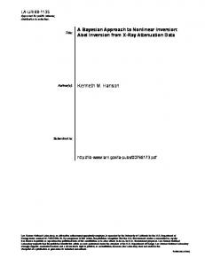
The value of 2,11 is set to 1 to fix the scale of ~. The following proper priors are used for the analysis: ~, = (Yl0, 711, 2/12)' ~ N(Y*, fl-/) with 3,* = (1, 1, 1) and l"~Yy1 = diag {0.01, 0.01, 0.01}; Oll - ~3(aeo, be) with a , = 1/2, b~ 1 = 0.01, XI~ll ~ ~ C ~ ( a ~ , b ~ ) with -1 * • * -t a ~ = 1/2, b,~ = 0.01, Vx,j ~ 3¢(Vxj, O~,xj ) with Vx, j = 0, and [i,,,x,j = 0.01 forj• = 1. . . . . • • * ' ' ' -1 • 4; Ax j ~ Ar(hx j, [Ix x j) with hx,j = 1, and O h x j = 0.01 forj = 2 . . . . . 4; 08 jj ~ ~¢~(as jj, bs,jj)'with as,i] = 1/2, b~,1 = 0.01 for j = 1 ~ : . . , 4. ' ' The results of the simulation are given in Tables 1-3. In these tables, the true parameters and the averages of the median, the mean and the standard deviation of the posterior distributions of the individual parameters over the 100 Monte Carlo replications are shown. These tables also give the 90 percent coverage for each parameter. In Bayesian analysis the coverage is computed by considering for each Monte Carlo replication whether the interval from the 5th to the 95th percentile in the distribution of the 2000 values of the Gibbs sampler covers the true parameter and then computing the proportion out of the 100 replications for which this event occurred. Tables 1 through 3 show close agreement between the true parameter and the average median and mean. Judging from the values of the average median and mean, the posterior distributions are already symmetric for n = 100. The coverage properties are acceptable for all parameters already for n = 100. Plotting the frequency estimate of the posterior distribution for individual parameters shows that these distributions are approximately normal even for the small sample size n = 100. As an example we consider the posterior distribution for the parameter of greatest interest in this specific nonlinear model, that is 3'12- The estimated posterior density is plotted using a histogram in Figure 1 and the k-nearest neighbor (kNN) smooth estimate (compare Loftsgaarden & Quesenberry 1965; and Hfirdle, 1990) in Figure 2. Figure 3 shows how the algorithm samples across the support of the posterior density from iteration to iteration indicating fast transition from one area of support to other areas. The regression model for the second data set includes two regressor variables and their interaction. The regression constant has been set to 0. Y~ = Yn~a + %2¢~z + %3~i~,2 + C,,

(98)

with ~ / ~ 3¢(0, O) and ~ / ~ de(0, '~11). • is now a 2 x 2 covariance matrix with elements {Oll, ~21, ~22}. The factor analytic model connecting ~i with five indicators xi is now

(99)

Xi -= A ~ i + ~i,

where ~i ~ X(0, Oa) and the regression constants v are set to 0. The matrix of factor loadings is given by a 5 × 2 matrix patterned as

A=|h31

0)1 0

.

(100)

O 8 is a diagonal matrix with O~ = {O~,11. . . . , O~,55}. The following proper priors are used for the analysis: 3, = (3'11, Y12, 3'13)' ~ ,~('Y*, l~v)

286

PSYCHOMETRIKA

TABLE 1

Averages of 100 M o n t e Carlo Replications Q u a d r a t i c Model, S a m p l e Size = 100 Gibbs: Cycles = 2000, B u r n - I n = 500 Metropolis: Cycles = 20 Parameter

True

Median

Mean

Std.Dev.

Cover

"7,0

0.5

0.4802

0.4747

0.1598

0.9500

")'11

1.0

1.0337

1.0378

0.1713

0.9300

712

-0.6

-0.6146

-0.6196

0.0747

0.8500

(I)11

1.4

1.3842

1.4050

0.2325

0.8900

~11

0.5

0.5117

0.5217

0.1001

0.9000

ul

-0.4

-0.4106

-0.4113

0.1285

0.9700

v2

-0.2

-0.2144

-0.2151

0.1174

0.9600

ua

0.2

0.1856

0.1852

0.1193

0.9500

u4

0.4

0.3752

0.3749

0.1097

0.9200

/~11 /~21

1.0

1.0000

1.0000

0.9

0.9132

0.9132

0.0567

0.8700

Aal

0.8

0.8034

0.8034

0.0719

0.9000

A41

0.7

0.6995

0.6995

0.0694

0.9200

O~la

0.2

0.1945

0.1984

0.0448

0.9200

0~22

0.2

0.2006

0.2042

0.0412

0.8900

®~3a

0.5

0.4989

0.5065

0.0802

0.8700

0~44

0.5

0.4910

0.4984

0.0773

0.9200

-

-

1.0000

with Y* = (1, 1, 1) and l-l~ 1 = diag {0.01, 0.01, 0.01}; (I) - ~lf-l(d¢l-lep, d+) where 1~¢ = diag {0.01, 0.01} and de = 2; ~11 - 9~3(a'I', b,i,) with a,i, = 1/2, b ~ 1 = 0.01; hxj g"( h x,j,12 h,x,j) wlthh x ,j = 1, andlq A, x,j = 0 •0 l f o r j = 2, 3, 5,@ 8,jj ~ ~ J a( &jj ,b 8,jj) with aa,jj = 1/2, b~,~ = 0.01 forj = 1, . . . , 5. The results of the Monte Carlo study are collected in Tables 4 through 6. The average means and medians of these tables show close agreement with the true parameters. The plots of the posterior density estimates of the interaction term 3'13 and the iteration behavior are similar to the plots shown for the previous example. 6.

Performance Regressed on Task Complexity and Goal Specificity

For empirical illustration we use data collected in 1990 from 158 police officers during a training course in Mtinster, Germany. Details of data collection are found in Holling

GERHARD ARMINGER AND BENGT O. MUTHEN

287

TABLE 2 Averages of 100 Monte Carlo Replications Quadratic Model, Sample Size = 250 Gibbs: Cycles = 2000, Burn-In = 500 Metropolis: Cycles = 20 Parameter

True

Median

Mean

Std.Dev.

Cover

710

0.5

0.4983

0.4962

0.0975

0.8600

711

1.0

1.0075

1.0089

0.1057

0.8600

7~2

-0.6

-0.6126

-0.6146

0.0446

0.8700

~n

1.4

1.3906

1.3989

0.1443

0.8800

II/11

0.5

0.5083

0.5121

0.0610

0.8500

vl

-0.4

-0.4018

-0.4024

0.0796

0.8800

u2

-0.2

-0.1981

-0.1982

0.0731

0.9000

ua

0.2

0.1942

0.1938

0.0745

0.8900

u4

0.4

0.3969

0.3968

0.0686

0.8900

All

1.0

1.0000

1.0000

--

1.0000

A21

0.9

0.9096

0.9096

0.0347

0.9200

~31

0.8

0.8051

0.8051

0.0444

0.8800

X41

0.7

0.7018

0.7018

0.0433

0.9000

0Sll

0.2

0.1986

0.2001

0.0276

0.9600

0s22

0.2

0.2000

0.2014

0.0255

0.9000

O~3a

0.5

0.4977

0.5006

0.0494

0.8900

0544

0.5

0.4996

0.5025

0.0484

0.9100

(1995). Background for the psychological theories to be tested are found in Early, Lee and Hanson (1990) and Holling. The dependent variable vI is performance, regressor variables are task complexity ~1, goal specificity ~2, and their interaction (~1~2). The corresponding model is a nonlinear regression model in latent variables ~i = 3"11~il + 3'12~i2 "{- 3"13(~i1~12) -I- ~i

(101)

with ~ - 3¢(0, $ ) where $ is a 2 × 2 covariance matrix with elements {¢P11,qb21, $22} and ffi ~ J~'(0, ~1I)- The proper priors for this part of the model are chosen as: 3' = (3"11, 3"12, 3"13)' - N(7*, l~r) with T* = (1, 1, - 1 ) . The value of - 1 is chosen since a negative interaction coefficient is expected theoretically. 1]~-1 = diag {0.01, 0.01, 0.01}. • w-l(d,l,g~a,, de) where f~,~ is a diagonal matrix with 12a,,11 = 1.9646 and f~,I,,Z2 = 0.6890.

288

PSYCHOMETRIKA

TABLE 3

Averages of 100 Monte Carlo Replications Q u a d r a t i c Model, S a m p l e Size = 500 Gibbs: Cycles = 2000, B u r n - I n = 500 Metropolis: Cycles = 20 Parameter

True

Median

Mean

Std.Dev.

Cover

71o

0.5

0.4848

0.4836

0.0686

0.8900

711

1.0

1.0147

1.0153

0.0739

0.8800

712

-0.6

-0.6047

-0.6056

0.0309

0.8800

(I)ll

1.4

1.3918

1.3957

0.1018

0.8200

~I/11

0.5

0.4983

0.5002

0.0417

0.9100

r'l

-0.4

-0.4100

-0.4101

0.0563

0.9100

u2

-0.2

-0.2099

-0.2097

0.0518

0.9000

ua

0.2

0.1887

0.1886

0.0528

0.8900

1,'4

0.4

0.3911

0.3910

0.0487

0.9200

"~11

1.0

1.0000

1.0000

--

1.0000

A21

0.9

0.9094

0.9094

0.0243

0.8600

•~al

0.8

0.8026

0.8026

0.0313

0.9100

A41

0.7

0.7019

0.7019

0.0305

0.8900

0~11

0.2

0.1994

0.2002

0.0192

0.8200

O~22

0.2

0.1955

0.1962

0.0174

0.8900

O~aa

0.5

0.5007

0.5022

0.0349

0.9500

0544

0.5

0.5026

0.5040

0.0342

0.9200

d o = 2; ~ u - ~(a,l,, b~) with a,I, = 1/2, b~,1 = 0.6782. The values of ~ and b,-ifl have been chosen from the variances of the reference indicators x 1, x4 and Yl of the latent variables ~1, ~2 and ~/. The indicator variables Yl, Y2, Y3 for the performance ~/are five point Likert scales with the questions A57A ("Is the amount of your work achieved during the last year (1) far below average to (5) far above average"), A57B ("Is the quality or precision of your work achieved during the last year (1) far below average to (5) far above average"), and A57E ("Is the fulfillment of your goals in your work achieved during the last year (1) far below average to (5) far above average"). The factor analytic model connecting the indicator variables Yl, Y2, Y3 with ~ is given by: Yi = Vy "[- A y l l i + e i

(102)

GERHARD ARMINGER AND BENGT O. MUTHEN

289

m mm m

C,

IIII

IIII ?

IIIIIIIIIII I I

~= 0

m m

8

m~

c~

E

[] m 0 c~

c! T

O~Z

OOZ

09&

O~&

~}ugnbBJj

i Og

i Oir

Z

!

g,

o

-1.2

-

1.0

-O.B

-0.6

FIGURE 2. Smooth estimate of the posterior density of ")112in the quadratic model.

_.........,.,---0.4

-0.2

0

q

¢o

{N

I

o

i

400

i

200

i 800

FIGURE 3.

Ileral~on

i 1000

I 1200

i 1400

Sample path of MCMC interactions for 712 of the quadratic model.

i 600

16 0

1800

2000

bO

m, Z

c

.o

Z ~q

Z

292

PSYCHOMETRIKA

TABLE 4

A v e r a g e s of 100 M o n t e Carlo R e p l i c a t i o n s I n t e r a c t i o n Model, S a m p l e Size = 100 Gibbs: Cycles = 2000, B u r n - I n = 500 Metropolis: Cycles = 20 Parameter

True

Median

Mean

Std.Dev.

Cover

711

0.8

0.8138

0.8176

0.1245

0.9200

712

1.7

1.8175

1.8476

0.2743

0.8200

7~3

0.5

0.5400

0.5514

0.1747

0.8700

(I)11

1.2

1.1522

1.1679

0.2179

0.8500

(I)21

0.1

0.0829

0.0857

0.0999

0.9400

(I)~2

0.7

0.6153

0.6298

O. 1638

0.8800

~n

0.6

0.6687

0.6858

0.1966

0.9000

An

1.0

1.0000

1.0000

--

1.0000

A21

0.7

0.7361

0.7361

0.0857

0.9100

A3~

-0.5

-0.5181

-0.5181

0.0773

0.9200

A42

1.0

1.0000

1.0000

--

1.0000

A52

1.6

1.8160

1.8160

0.2862

0.8400

@sll

0.2

0.2130

0.2195

0.0887

0.9000

Os22

0.3

0.2885

0.2921

0.0626

0.8900

0s33

0.4

0.4084

0.4142

0.0656

0.9600

0~4 4

0.5

0.5250

0.5331

0.1000

0.8400

Os~s

0.6

0.5321

0.5396

0.1844

0.8800

with Ei - d¢(O, 0~) and the parameter specification

,:'t, (1 t

Vy = | Vy,21, Ay = \ l]y,3]

h,,n , O~ = diag {O~.., 08.22, 0°.33}.

\/~'y,31

(103)

/

The value of Ay,11 is set to 1 to fix the scale of ~/. The proper priors for this part of the model are specified as: Vy,j ~ )¢(Vyj, f~,,y,]) where Vyy = O, and l~,ylj = 0.01 forj = 1, * '-1 '' 2, 3; Avil . . . d~'(hvil, . . * . ~'~)t.vil) where' A,,q:, = 1, and lqx,:,,;]j = 0.01 for j• -- 2, 3," @~,,;; ,9~3(ae,jj, be,jj) witia ae,jj =' 1/2, b~,1. = '0.01 for j = 1,. '.., 3. The indicator variables x 1, x 2, x 3 for task complexity ~1 are A18 ("How many of your ~

293

GERHARD ARMINGER AND BENGT O. MUTHt~N

TABLE 5

Averages of 100 Monte Carlo Replications I n t e r a c t i o n Model, S a m p l e Size = 250 Gibbs: Cycles = 2000, B u r n - I n = 500 Metropolis: Cycles = 20 Parameter

True

Median

Mean

Std.Dev.

Cover

711

0.8

0.8004

0.8017

0.0738

0.9100

"h2

1.7

1.6925

1.6992

0.1375

0.9500

")'13

0.5

0.4971

0.5001

0.0913

0.9600

(1~11

1.2

1.1687

1.1751

0.1327

0.9200

(I)21

0.1

0.1041

0.1053

0.0654

0.8900

(I)22

0.7

0.6698

0.6754

0.1036

0.8800

~11

0.6

0.6728

0.6792

0.1138

0.8300

An

1.0

1.0000

1.0000

--

1.0000

A21

0.7

0.7087

0.7087

0.0483

0.9100

/~31

-0.5

-0.5055

-0.5055

0.0452

0.9000

A42

1.0

1.0000

1.0000

--

1.0000

A52

1.6

1.6651

1.6651

0.1384

0.8700

0511

0.2

0.1930

0.1947

0.0532

0.8300

0522

0.3

0.3003

0.3019

0.0379

0.8900

0533

0.4

0.3898

0.3919

0.0388

0.9000

0544

0.5

0.5058

0.5090

0.0590

0.8800

0555

0.6

0.5538

0.5567

0.1061

0.8300

main tasks are the same from day to day" ranging from (1) almost all to (5) almost none), A19 ("Are the daily situations in which you have to fulfill your tasks (1) very much the same to (5) usually very different"), and A28 ("Are the daily problems which you have to solve to fulfill your tasks (1) very much the same to (5) usually very different"). The indicator variables x4, x5, x6 for goal specificity ~2 are A45 ("Are the performance requirements set by your superior officer (1) very unclear to (5) very clear"), A55A ("Are the goals set for your work always clear and specific" ranging from (1) not true at all to (5) almost always true), and B09 ("Are the specific goals for your work (1) very unclear to (5) very clear"). The factor analytic model connecting the indicator variables xl, x2, x 3 with ~1 and x4, x 5, x 6 with ~2 is:

PSYCHOMETRIKA

294

TABLE 6 Averages of 100 Monte Carlo Replications Interaction Model, Sample Size = 500 Gibbs: Cycles = 2000, Burn-In = 500 Metropolis: Cycles = 20 Parameter

True

Median

Mean

Std.Dev.

Cover

")'11

0.8

0.7969

0.7975

0.0505

0.8500

712

1.7

1.7153

1.7188

0.0941

0.9100

7a3

0.5

0.4983

0.4997

0.0616

0.9000

~11 (I)21

1.2

1.1997

1.2030

0.0952

0.9000

0.1

0.1073

0.1079

0.0473

0.9300

~22

0.7

0.6858

0.6889

0.0729

0.8500

q/n

0.6

0.6429

0.6459

0.0779

0.9100

A11

1.0

1.0000

1.0000

--

1.0000

A2a

0.7

0.7010

0.7010

0.0331

0.8900

),31

-0.5

-0.4966

-0.4966

0.0310

0.8900

),42

1.0

1.0000

1.0000

--

1.0000

),52

1.6

1.6363

1.6363

0.0903

0.8600

O511

0.2

0.1995

0.2006

0.0375

0.9100

0522

0.3

0.3026

0.3034

0.0267

0.9000

O~33

0.4

0.3927

0.3938

0.0275

0.8500

0544

0.5

0.5013

0.5027

0.0405

0.8900

0555

0.6

0.5759

0.5773

0.0714

0.8700

xi = vx + Ax~i + 6i

(104)

with 6i - N(0, @8) and the parameter specification

Vx,2|

\ Px,5] '~1)x,6l

l O

hx,21

0

hx31

0

0

Ax5z

0

Ax:62

, 08 = diag {®~,11. . . . . ®~,66}.

(105)

295

GERHARD ARMINGER AND BENGT O. MUTHt~N

Again, the values of hx,11 and Ax,42 a r e set to 1 to fix the scales of ~1 and ~2. The proper priors for this part of the model are specified as: Vx,k ~ N(~'*,k, l~,,,x,k) where Vx,k = 0, and l)v,x, k - 0.01 for k - 1. . . . ,6, )tx,kl ~ .]f()tx,kl , ~'~)~,x,kl) where A.x,kl -- 1, and UtA,x,kl = • * -1 0.01 for k -- 2, 3; Axk 2 ~ .~(Axk 2, l'~Xx,k2) where Axk2 = 1, and ~A,xk2 = 0.01 for k 5, 6; ®~,kk -- ~3(aS,kk, bs,kk) with a~,kk = 1/2, b~,kk = 0.01 for k = 1, . . . , 6. The analysis has been performed with a burn in phase of 500 Gibbs iterations and 2000 additional Gibbs iterations and 50 Metropolis-Hastings iterations within each Gibbs cycle to estimate the posterior distribution. To check convergence we have also used 20000 Gibbs cycles and have found identical results. We first report in Table 7 median, mean and standard deviation of the posterior distributions of the individual parameters of a linear regression model (without the interaction term ~1~2) as well as of the non-linear regression model including the interaction term with the additional parameter 713. While most of the medians and means of most parameters show close agreement, the values of 711 and ]t12are somewhat higher in the non-linear regression model. The sign of the interaction parameter 713 is negative, the standard deviation indicates that the interaction term may be considered as significantly different from 0 using a conventional 95 percent coverage. The median coefficient of determination R 2 increases from 0.1016 in the linear model to 0.2750 in the non-linear model indicating a higher predictive power of the nonlinear model. Substantively, this result implies that increases in task complexity and in goal specificity predict an increase in performance, but the increase is dampened by the negative sign of the interaction term. For the interaction parameter 713 we plot the smoothed (kNN) density estimate in Figure 4 and the sample path of the MCMC algorithm in Figure 5. In Table 8 the results are reported for the factor analytic model for (Ya, Y2, Y3) as indicators for the performance 7. The results agree closely for the linear and the non-linear regression model implying that the relations in the factor analytic model for the performance are not changed by the underlying regression model for 7. Similar results hold for the factor analytic model c o n n e c t i n g (Xl, x2, X3) to task complexity ~a and (x4, xs, x6) to goal specificity ~2" -1

_

_

.

*

7.

*

_

-1

Conclusion

We have formulated a nonlinear latent variable model including quadratic functions and interactions of latent regressors. Estimation of model parameters using conventional covariance structure analysis is almost impossible yielding unwieldy mean and covariance structures and cumbersome numerical algorithms. Putting the nonlinear latent variable model in a Bayesian framework allows the use of the Gibbs sampler to estimate the posterior distributions of the parameters and the latent variables given the data. The Bayesian framework also allows the incorporation of prior information by specifying prior distributions for the model parameters. The application of the Gibbs sampler is complicated by the fact that no closed mathematical form of the distribution of the latent variables could be found. Therefore, the M-H algorithm is used within iterations of the Gibbs sampler. The proposed model and the numerical algorithms are illustrated by two simulation studies and an empirical example analyzing the possibly non-linear dependence of performance on task complexity and goal specificity. In the future, further checks of the behavior of the proposed algorithm and an analysis of the sensitivity of the results to the specification of strong priors will have to be performed.

296

PSYCHOMETRIKA

TABLE 7 Linear and Non-linear Regression Model Gibbs: Cycles = 2000, Burn-In = 500 Metropolis: Cycles = 50 Linear regression model

Non-linear regression model

Parameter

Median

Mean

Std.Dev.

Median

Mean

Std.Dev.

711

0.0921

0.0931

0.0540

0.1323

0.1336

0.0619

712

0.3649

0.3745

0.2078

0.6099

0.6304

0.2382

0.4131

-0.4363

0.1979

713

.

.

.

.

~ax

1.2575

1.2716

0.2506

1.1491

1.1685

0.2321

~21

-0.0164

-0.0153

0.0525

-0.0233

-0.0239

0.0538

¢22

0.1827

0.1950

0.0687

0.1983

0.2072

0.0699

~H

0.3403

0.3438

0.0760

0.2902

0.2961

0.0695

R~

0.1016

0.1129

0.0706

0.2750

0.2797

0.1157

TABLE 8 Factor Analytic Model for Performance Gibbs: Cycles -- 2000, Burn-In --- 500 Metropolis: Cycles - 50 Linear regressio n model

Non-linear regression model

Parameter

Median

Mean

Std.Dev.

Median

Mean

Std.Dev.

uy,1

4.3197

4.3215

0.0652

4.3191

4.3174

0.0718

uy,2

4.3534

4.3527

0.0574

4.3521

4.3505

0.0623

uy,3

4.2219

4.2211

0.0583

4.2194

4.2158

0.0620

Av,ll

1.0000

1.0000

--

1.0000

1.0000

--

Av,21

0.9040

0.9174

0.1211

0.8839

0.8915

0.1019

Av,31

0.9403

0.9522

0.1181

0.9049

0.9102

0.1004

Odl

0.3135

0.3158

0.0525

0.3015

0.3028

0.0482

O~,22

0.2063

0.2070

0.0409

0.2037

0.2050

0.0356

O~,33

0.1821

0.1819

0.0411

0.1883

0.1902

0.0359

297

GERHARD ARMINGER AND BENGT O. MUTHEN

~ 6,It

o

C~

¢3

o'~ 9"~ Z'£ g'i~ ~z o!~ 9"t Z!L ~t'o s,~o 0"o AI~!SueO - N N > I

,q

-I.2 o

-0.8

-0.4

-0.0

0.4

g o

•

J,

g~

86E

V~I~IJ~HI~IOHDXSd

299

GERHARD ARMINGER AND BENGT O. MUTHI~N

TABLE 9 Factor Analytic Model for Task Complexity and Goal Specificity Gibbs: Cycles = 2000, Burn-In = 500 Metropolis: Cycles = 50 Linear regression model

Non-linear regression model

Parameter

Median

Mean

Std.Dev.

Median

Mean

Std.Dev.

v~,l

2.6146

2.6195

0.1188

2.6137

2.6119

0.1161

vx,2

2.8971

2.9050

0.1103

2.8950

2.8920

0.1106

v~,3

2.7570

2.7588

0.0924

2.7491

2.7496

0.0929

vx,4

4.0758

4.0735

0.0694

4.0737

4.0735

0.0690

vx,5

4.3325

4.3305

0.0566

4.3302

4.3310

0.0582

v~,6

3.8182

3.8163

0.0845

3.8135

3.8147

0.0893

Ax,11

1.0000

1.0000

--

1.0000

1.0000

--

A~,21

1.0117

1.0272

0.1348

1.0985

1.1060

0.1325

Ax,31

0.6590

0.6622

0.0886

0.6735

0.6795

0.0914

A~,42

1.0000

1.0000

--

1.0000

1.0000

--

Ax,s2

0.8117

0.8413

0.2813

0.9112

0.9312

0.2716

A~,62

1.5850

1.7142

0.6228

1.2884

1.3140

0.3287

0~,11

0.7218

0.7259

0.1553

0.8099

0.8127

0.1412

08,22

0.4570

0.4457

0.1512

0.3443

0.3524

0.1374

O~,33

0.7287

0.7361

0.1059

0.7516

0.7585

0.1054

06,44

0.5357

0.5396

0.0915

0.5092

0.5110

0.0796

O~,5~

0.3742

0.3694

0.0750

0.3377

0.3386

0.0615

O~,6~

0.6961

0.6330

0.2812

0.8334

0.8357

0.1369

References Anderson, T. W. (1984). An Introduction to multivariate statistical analysis (2nd ed.). New York: Wiley. Arminger, G., & Schoenberg, R. J. (1989). Pseudo maximum likelihood estimation and a test for misspecification in mean and covariance structure models. Psychometrika, 54, 409-425. Arminger, G., Wittenberg, J., & Schepers, A. (1996). MECOSA3 User Guide. Friedrichsdorf, Germany: ADDITIVE GmbH. Arnold, S. F. (1993). Gibbs Sampling. In C. R. Rao (Ed.), Handbook of statistics (Vol. 9, pp. 599-625). Amsterdam: North Holland. Besag, J., Green, P., Higdon, D., & Mengersen, K. (1995). Bayesian computation and stochastic systems. Statistical Science, 19(1), 3-66. Box, G. E. P., & Tiao, G. C. (1973). Bayesian inference in statistical analysis. Reading: Addison-Wesley. Browne, M. W. (1984). Asymptotic distribution-free methods for the analysis of covariance structures. British Journal of Mathematical and Statistical Psychology, 37, 62-83.

300

PSYCHOMETRIKA

Carlin, B. P., & Louis, T. A. (1996). Bayes and empirical bayes methods for data analysis. London: Chapman & Hall. Casella, G., & George, E. I. (1992). Explaining the Gibbs sampler. The American Statistican, 46, 167-174. Chib, S., & Greenberg, E. (1995). Understanding the Metropolis-Hastings algorithm. The American Statistican, 49(4), 327-335. Chib, S., & Greenberg, E. S. (1996). Markov chain Monte Carlo simulation methods in econometrics. Econometric Theory, 12(3), 409-431. Early, P. C., Lee, C., & Hanson, L. A. (1990). Joint moderating effects of job experience and task component complexity: relations among goal setting, task strategies, and performance. Journal of Organizational Behavior, 1I, 3-15. Gelfand, A. E , & Smith, A. F. M. (1990). Sampling-based approaches to calculating marginal densities. Journal of the American Statistical Association, 85, 398-409. Gelman, A., Carlin, J. B., Stern, H. S., & Rubin, D. B. (1995). Bayesian data analysis. London: Chapman & Hall. Gelman, A., & Rubin, D. B. (1992). Inference from Iterative Simulation Using Multiple Sequences (with discussion). Statistical Science, 7, 457-511. Geman, S., & Geman, D. (1984). Stochastic relaxation, Gibbs distribution and the Bayesian restoration of images. IEEE Transactions on Pattern Analysis and Machine Intelligence, 6, 721-741. Gilks, W. R., Richardson, S., & Spiegelhalter, D. J. (1996). Markov chain Monte Carlo in practice, London: Chapman and Hall. H~irdle, W. (1990). Applied nonparametric regression. Cambridge, MA: Cambridge University Press. Hastings, W. K. (1970). Monte Carlo sampling methods using Markov chains and their applications. Biometrika, 57, 97-109. Hayduk, L. A. (1987). Structural equation modeling with LISREL: Essentials and advances. Baltimore, MD: Johns Hopkins Press. Hobert, J. P., & Casella, G. (in press). The effect of improper priors on Gibbs sampling in hierarchical linear mixed models. Journal of the American Statistical Association. Holling, H. (1995). Goal setting and performance. Unpublished manuscript, Universit/~t Mfinster, Department of Psychology, Germany. J6reskog, K. G., & S6rbom, D. (i993). LISREL 8." Structural equation modeling with the SIMPLIS command language. Hillsdale, NJ, Lawrence Earlbaum Associates. J6reskog, K. G., & Yang, F. (1996). Nonlinear structural equation models: The Kenny-Judd model with interaction effects. In G. A. Marcoulides, & R. E. Schumacker (Eds.), Advanced structural equation modeling techniques (pp. 57-88). Hillsdale, NJ, Lawrence Erlbaum Associates. Kenny, D., & Judd, C. M. (1984). Estimating the nonlinear and interactive effects of latent variables. Psychological Bulletin, 96, 201-210. Lawley, D. N., & Maxwell, A. E. (1971). Factor analysis as a statistical method. London: Butterworth. Lee, S. Y. (1991). A Bayesian Approach to Confirmatory Factor Analysis. Psychometrika, 46, 153-160. Lindley, D. V., & Smith, A. F. M. (1972). Bayes estimates for the linear model (with discussion). Journal of the Royal Statistical Society, Series B, 34, 1-41. Loftsgaarden, D. O., & Quesenberry, G. P. (1965). A nonparametric estimate of a multivariate density function. Annals of Mathematical Statistics, 36, 1049-1051. MacEachern, S. N., & Berliner, M. L. (1994). Subsampling the Gibbs sampler. The American Statistican, 48, 188-190. Metropolis, N., Rosenbluth, A. W., Rosenbluth, M. N., Teller, A. H., & Teller, E. (1953). Equations of state calculations by fast computing machines. Journal of Chemical Physics, 21, 108%1091. Mfiller, P. (1994). Metroplis Based Posterior Integration Schemes. Unpublished manuscript, Duke University, Durham. Muth6n, B. O. (1988). LISCOMP--Analysis of linear structural equations with a comprehensive measurement model. Mooresville: Scientific Software. Press, S. J., & Shigemasu, K. (1989). Bayesian inference in factor analysis. In L. Gleser, M. D. Perlman, S. J. Press, & A. R. Sampson (Eds.), Contributions to probability and statistics (pp. 271-287). New York: Springer Verlag. Ritter, C., & Tanner, M. A. (1992). Facilitating the Gibbs sampler: The Gibbs stopper and the Griddy-Gibbs sampler. Journal of the American Statistical Association, 87, 861-868. Rubin, D. B. (1991). EM and Beyond. Psychometrika, 56, 241-254. Tanner, M. A. (1993). Tools for statistical inference (2nd ed.). Heidelberg and New York: Springer Verlag. Tierney, L. (1994). Markov chains for exploring posterior distributions (with Discussion). Annals of Statistics, 22, 1701-1762. Manuscript received 12/8/95 Final version received 12/10/97