A BAYESIAN STEPWISE MULTIPLE TESTING PROCEDURE By Sanat K. Sarkar 1 and Jie Chen Temple University and Merck Research Laboratories Abstract Bayesian testing of multiple hypotheses often requires consideration of all configurations of the true and false null hypotheses, which is a difficult task when the number of hypotheses is even moderately large. In this article, a Bayesian stepwise approach is proposed. After ordering the null hypotheses in terms of their marginal Bayes factors, a determination is made of all possible configurations of true and false ordered null hypotheses. The most plausible configuration is then tested in a stepwise manner starting with the intersection of all the null hypotheses. The present Bayesian approach provides considerable reduction in the size of the set of families within which we restrict our posterior search for the “right” family of true and false null hypotheses, from 2k to only k + 1, given k null hypotheses. The hierarchical prior structure is considered in general. The stepwise Bayes factors are derived in situations involving point null hypotheses as well as those arising in one-sided testing problems under normal distributional settings. Our procedure when applied to three different examples results in conclusions that are similar to those obtained using an analogous frequentist approach.
1. Introduction.
Simultaneous testing of multiple null hypotheses, simply
referred to as multiple testing, is a common inference problem in many statistical experiments. For instance, in pharmaceutical investigations of the efficacy of an experimental drug, the statistical assessment of the drug’s superiority over existing drugs or over placebo on multiple endpoints is generally carried out through 1 Research
was supported in part by NSA Grant MDA-904-01-10082
AMS 2000 subject classification. Primary 62J15, 62F15 Key words and phrases: Hierarchical prior, simultaneous testing, multiple hypotheses, stepwise Bayes factor, marginal Bayes factor.
1
a multiple testing formulation. Such testing is often performed using frequentist stepwise multiple test procedures in which the ordered test statistics or the associated p-values are compared with a set of critical values in a stepwise fashion toward identifying the set of true and false null hypotheses. The critical value used in each step incorporates the decision made in the preceding step. Therefore, they provide better control of the familywise error rate, and hence are more powerful, compared to a single-step procedure where the determination of true and false hypotheses are made by simply comparing each test statistic or the corresponding p-value with a single critical value. A considerable amount of research has taken place on stepwise multiple testing from frequentist’s viewpoint (Hochberg and Tamhane 1987; Dunnett and Tamhane 1991; Dunnett and Tamhane 1992; Finner 1993; Westfall and Young 1993; Hsu 1996; Liu 1996; Liu 1997; Holm 1999), with many of the proposed methodologies having been incorporated into statistical packages (Westfall and Tobias 1999; Westfall, Tobias, Rom, Wolfinger, and Hochberg 1999). Basically, there are two types of frequentist stepwise multiple testing procedures that are most commonly used – step-up and step-down procedures. After ordering the hypotheses according to increasing values of their test statistics or p-values, a step-down procedure starts with testing the most significant hypothesis and continues until an acceptance occurs or all the hypotheses are rejected. On the other hand, a step-up test starts with testing the least significant hypothesis and continues until a rejection occurs or all the hypotheses are accepted. A generalized version of step-up and step-down procedures has received some attention recently (Tamhane, Liu, and Dunnett 1998; Sarkar 2002). What would be a Bayesian analog of a frequentist stepwise testing? This seems to be an interesting question to answer as no such analog is yet available in the literature. We develop in this article a Bayesian stepwise procedure for multiple testing of null hypotheses that are non-hierarchical, i.e., no hypothesis is implying any other. The procedure involves two main steps, specification of a set of target families of true and false null hypotheses and a stepwise search for the most plausible one of these families. Given data and prior specifications of the parameters, an ordering is established among the null hypotheses according to increasing values 2
of their marginal Bayes factors, which will guide the determination of the target families. Once these target families are formed, the stepwise search is carried out using stepwise Bayes factors toward identifying the most plausible family.
Given k null hypotheses, the total number of target families is k + 1. The idea used in configuring these different families is that, among all families with r false and k − r true null hypotheses, the one in which the first r ordered null hypotheses are false and the last k − r ordered null hypotheses are true is the most plausible, where the ordering of hypotheses is made according to an increasing magnitude of their marginal Bayes factors. The stepwise search begins with the target family with no false hypotheses. The strength of evidence of this family against all other families is checked by computing the Bayes factor of the intersection of the hypotheses in the family. If the evidence is strong, the search stops by declaring all of the k null hypotheses to be true; otherwise, it declares the null hypothesis with the smallest marginal Bayes factor to be false and goes to the next step. The next step involves the rest k target families where the null hypothesis rejected in the beginning step is considered false. Within this group of families, the evidentiary strength of the family in which the previously rejected null hypothesis is false and the rest are true is assessed by the Bayes factor, conditional on this group, of the corresponding intersection hypothesis. If this evidence is strong, the search stops by declaring the null hypothesis with the smallest marginal Bayes factor to be false and the rest to be true; otherwise, it continues to the next step. These conditional Bayes factors are referred to as stepwise Bayes factors in this article. The search continues until a stepwise Bayes factor provides a strong evidence for the corresponding intersection hypothesis. There is an operational similarity between our proposed Bayesian stepwise procedure and classical step-down multiple test procedure. Target families are also formed, of course, in terms of ordered test statistics or p-values, in classical step-down procedure using similar idea. Also the search for the statistically most significant target family in classical step-down procedure proceeds from the family with no false hypotheses toward those with higher number of false hypotheses. In this sense, our proposed method is a Bayesian step-down multiple test procedure. 3
It is important to emphasize certain positive features of the proposed method relative to those that exist in the Bayesian literature. Multiple testing is typically viewed as a model selection problem when it is approached from a Bayesian perspective, with different configurations of true and false null hypotheses being the competing models. The existing Bayesian model selection methods when applied to such a formulation of multiple testing, however, have to search for the “right” model or configuration within the set of all 2k configurations of true and false null hypotheses (Bertolino, Piccinato, and Racugno 1995; Berger and Pericchi 1996; Berger 1999; Berger and Pericchi 2001, and references therein). This is an increasingly difficult task when k becomes large. In our method, on the other hand, the initial process of specifying the target families, allows us to disregard configurations, which we call families, that are undesirable in the sense of being relatively less evident a posteriori. This provides considerable reduction in the size of the set of families within which we restrict our posterior search for the “right” family of true and false null hypotheses, from 2k to only k + 1. Because of this, the computational task greatly reduced. Another existing Bayesian approach to multiple testing is to use simultaneous credible regions (Gelman and Tuerlinckx 2000). As opposed to such a single-step Bayesian approach, where the test for a given family does not depend on those for the others, our proposed step-down method offers a systematic improvement of the search for the “right” family by incorporating information gathered at every step. This seems to be a more effective way of adjusting for the multiplicity in the present multiple testing problem; see Berry (1988); Breslow (1990); and Berry and Hochberg (1999) for discussions on the general issue of handling multiplicity from Bayesian viewpoint. The proposed Bayesian step-down procedure is developed for simultaneous testing of multiple point as well as one-sided null hypotheses against the corresponding complementary alternatives. For these types of null and alternative hypotheses involving parameters of a number of different populations, formulas are derived for both marginal and stepwise Bayes factors based on a dataset that consists of independent samples from the populations and a prior under which the parameters are independent conditional on some hyper-parameter. The hierarchical structure 4
of the prior also provides a way of adjusting for multiplicity. These formulas are further developed in detail for situations where means of several normal populations are simultaneously compared with a known value or with the mean of another population, assuming a common unknown variance of the populations. The scope of our method is illustrated by applying it to three datasets, one in Romano (1977, p. 248), one in White and Froeb (1980) and the other in Steel and Torrie (1980). The formulas for simultaneous testing of multiple point null hypotheses against one-sided alternatives have been developed in Chen and Sarkar (2002). A number of other papers, many of them recently, have appeared in the literature where Bayesian approach has been taken to address some problems in multiple comparisons. Duncan (1965) proposed a Bayesian decision-theoretic approach for multiple comparisons, in which a decision is made using relative magnitudes of losses due to Type I and Type II errors. An extension of this idea can be found in Waller and Duncan (1969) who used a hyper-prior distribution for the unknown ratio of between-to-within variances. Shaffer (1999) modified Duncan’s procedure (semi-Bayesian) and found considerable similarity in both risk and average power between this modified procedure and the FDR-controlling procedure due to Benjamini and Hochberg (1995). Tamhane and Gopal (1993) derived Bayes decision rules for comparing treatments with a control under an additive overall loss function with either constant or linear loss functions for component losses. Westfall, Johnson, and Utts (1997) studied prior probability adjustment to account for multiple hypotheses and showed that the adjusted posterior probabilities correspond to Bonferroni adjusted p-values. Gopalan and Berry (1998) proposed a Bayesian multiple comparisons procedure for means in terms of posterior probabilities of all possible hypotheses of equality and inequality among means under Dirichlet process priors. The paper is organized as follows. Section 2 provides some preliminaries. Section 3 describes the proposed Bayesian stepwise procedure with necessary formulas for simultaneous testing of multiple point as well as one-sided null hypotheses against the corresponding complementary alternatives. Further developments of the formulas for normal populations using priors recommended in Berger, Boukai, and Wang 5
(1997a); Berger, Boukai, and Wang (1997b); and Berger, Boukai, and Wang (1999) are given in Section 4 before applying them to three data sets. The article is concluded in Section 5 with some remarks and discussion. Proofs of some formulas are presented in the Appendix.
2. Preliminaries.
Suppose that we have a data set X = {X1 , · · · , Xk } con-
sisting of independent samples Xi : ni × 1, i = 1, · · · , k, from k populations and that Xi has the following density f (xi |θi ) =
ni Y
f (xij |θi ),
j=1
i = 1, . . . , k, where θ = (θ1 , . . . , θk ) ∈ Ω ⊂ j. In other words, among all kr possible configurations of the k null hypotheses with r of them having weak and k −r having ¯ (1) · · · H ¯ (r) H(r+1) · · · H(k) . strong evidences, the most plausible configuration is H This leads us to the consideration of the following set of k + 1 families ©
ª © ª © ª ¯ (1) , H(2) , . . . , H(k) , . . . , H ¯ (1) , . . . , H ¯ (k−1) , H(k) , H(1) , . . . , H(k) , H
©
ª ¯ (1) , . . . , H ¯ (k) , H
within which we will restrict our search for the most plausible family of true and false null hypotheses. For this, let us define ( r ) ( k ) \ \ \ ¯ (i) H H(i) , H (r) = i=1
i=r+1
¯ 0 = Ω. Also, the Bayes factor, called the stepwise Bayes for r = 0, 1, . . . , k with H factor, of H (r) to any of H (r+1) , . . . , H (k) is defined as Pk π(H (i) ) P (H (r) |X) B (r) = Pk · i=r+1 (r) , (i) π(H ) i=r+1 P (H |X) where π(H (r) ) is the prior probability of H (r) , r = 0, 1, . . . , k − 1. The Bayesian step-down procedure for selecting the most plausible target family then proceeds as follows: Step 0. Start with r = 0, i.e., the intersection of all the k null hypotheses, calculate B (0) . If B (0) > c, then accept H (0) = ∩ki=1 H(i) and stop; if B (0) ≤ c, then reject H(1) go to the next step. ··· Step r. Calculate B (r) . If B (r) > c, then accept H (r) and stop; if B (r) ≤ c, then reject all H(i) for i ≤ r + 1 and go to the next step. ··· Step k-1. Calculate B (k−1) . If B (k−1) > c, then accept H (k−1) and stop; if B (k−1) ≤ c, then reject all H(i) for i ≤ k. 9
In each step of the above procedure, the stepwise Bayes factor of the hypothetical target family to any of the remaining target families is calculated and compared with a predetermined constant c. In testing a single hypothesis against an alternative using Bayes factor, different authors (Berger, Brown, and Wolpert 1994; Berger, Boukai, and Wang 1997b) have suggested using different constants for rejecting the null hypothesis. We will, however, adopt the principle of Berger, Boukai, and Wang (1997b) and use 1 for the constant c. This makes sense because a Bayes factor less than or equal to 1 simply would imply that the null model is less likely to be true as compared to the alternative model. Notice that a rejection of the intersection of null hypotheses suggests that at least one of the individual null hypotheses is not true; which naturally leads us to reject the null hypothesis with the smallest posterior probability or marginal Bayes factor. 3.2. Testing Multiple Point Null Hypotheses. We will derive in this subsection the formulas necessary to perform the proposed procedure for simultaneous testing of point null hypothesis Hi : θi = θi0 , i = 1, . . . , k, against the corresponding ¯ i : θi 6= θi0 , i = 1, . . . , k. Since we have point null complementary alternatives H hypotheses, we cannot use a continuous prior density. The most common approach ¯ i the density in this case is to assign Hi a positive probability πi0 , while giving H (1−πi0 )g1 (θi |λ), conditional on λ, with g1 (θi |λ) being a proper prior (Berger 1985). Note that θi0 can be a known, fixed number or an unknown parameter with a prior distribution. We will consider in the following both cases with known and unknown θi0 . For each θi , the conditional prior given λ is π1 (θi |λ) = πi0 I(θi = θi0 ) + (1 − πi0 )g1 (θi |λ)I(θi 6= θi0 ). If θi0 is known, the posterior probability of Hi given X is Z " (3.4)
−1
P (Hi |X) = [m(X)]
k
πi0 f (Xi |θi0 )
Y(−i) n πj0 f (Xj |θj0 ) j=1
# o +(1 − πj0 )f (Xj |λ) π2 (λ)dλ, ∗
10
where Z m(X) =
k Y ©
ª πj0 f (Xj |θj0 ) + (1 − πj0 )f ∗ (Xj |λ) π2 (λ)dλ,
j=1
Z f ∗ (Xj |λ) =
f (Xj |θj )g1 (θj |λ)dθj ,
j = 1, . . . , k,
k
and
Y(−i)
means that the product is taken over j from 1 to k, excluding i. Note
j=1
that, for each j, the density f (Xj |θj ) may also involve the parameter λ, as in the case of a normal with unknown variance (Section 4). To avoid notational complications in obtaining the formula for P (H (r) |X), the posterior probability of H (r) given X, we will assume here and also in the rest of the paper that Hi is the ith ordered hypothesis H(i) , for i = 1, . . . , k. Then we have, Z "Y r © ª (r) −1 (3.5) (1 − πi0 )f ∗ (Xi |λ) P (H |X) = [m(X)] i=1 k Y ©
πi0 f (Xi |θi0
ª
# π2 (λ)dλ,
i=r+1
using which the stepwise Bayes factor for testing H (r) can be obtained as follows: ! Ã j k X Y 1 − πi0 P (H (r) |X) (r) (3.6) B = Pk . · (j) |X) πi0 j=r+1 P (H j=r+1 i=r+1 When λ = (λ1 , λ2 ) is known, the (3.6) can be expressed in terms of marginal Bayes factors:
(3.7) B (r) =
k X j=r+1
Ã
!−1 k à j ! j Y X Y 1 − πi0 1 1 − πi0 . π B πi0 i0 i i=r+1 j=r+1 i=r+1
If θ10 = · · · = θk0 ≡ θ0 , where θ0 is an unknown parameter corresponding to some other commonly referenced group such as a control group, and let f (X0 |θ0 ) denote the density function of the observed data X0 and π1 (θ0 |λ) the prior pdf of θ0 for the control group, then the posterior probability of Hi given X becomes k Z ·Z Y(−i) © −1 (3.8) P (Hi |X) = [m0 (X)] πj0 f (Xj |θ0 ) f (X0 |θ0 )πi0 f (Xi |θ0 ) j=1
¸ ª +(1 − πj0 )f (Xj |λ) π1 (θ0 |λ)dθ0 π2 (λ)dλ, ∗
11
where Z ·Z m0 (X) =
f (X0 |θ0 )
k n Y πj0 f (Xj |θ0 ) j=1
¸ o +(1 − πj0 )f (Xj |λ) π1 (θ0 |λ)dθ0 π2 (λ)dλ. ∗
The posterior probability of H (r) given X is ½Y Z · r f (X0 |θ0 ) (3.9) P (H (r) |X) = [m0 (X)]−1 (1 − πj0 )f ∗ (Xj |λ) j=1 k Y
¾
¸ πj0 f (Xj |θ0 ) π1 (θ0 |λ)dθ0 π2 (λ)dλ.
j=r+1
3.3. Testing Multiple One-Sided Null Hypotheses. Consider now the problem ¯ i : θi > θi0 , simultaneously for i = 1, . . . , k. Let of testing Hi : θi ≤ θi0 versus H the prior pdf of θi , conditional on λ, be π1 (θi |λ), i = 1, . . . , k. If θi0 is known, the posterior probability of Hi and H (r) given X are given by: Z · (3.10)
∗
−1
k
f0∗ (Xi |λ)
P (Hi |X) = [m (X)]
Y(−i) ©
¸ ª f (Xj |λ) π2 (λ)dλ ∗
j=1
and (3.11)
P (H
(r)
∗
−1
|X) = [m (X)]
Z ·Y r ©
ª f1∗ (Xj |λ)
j=1 k Y ©
ª
¸
f0∗ (Xj |λ)
π2 (λ)dλ,
j=r+1
respectively, where m∗ (X) =
Z ·Y k ©
¸ ª f ∗ (Xj |λ) π2 (λ)dλ,
j=1
Z f ∗ (Xj |λ) =
f (Xj |θj )π1 (θj |λ)dθj ,
Z f0∗ (Xj |λ) =
f (Xj |θj )π1 (θj |λ)dθj , θj ≤θj0
and Z f1∗ (Xj |λ) =
f (Xj |θj )π1 (θj |λ)dθj . θj >θj0
12
The stepwise Bayes factor for H (r) is then obtained from the following formula: Pk π0 (H (i) ) P (H (r) |X) (r) (3.12) , B = Pk · i=r+1 (r) (i) π0 (H ) i=r+1 P (H |X) where π0 (H (r) ) =
Z ·Y r ½Z i=1
π1 (θi |λ)dθi
¾ Y ½Z k
θi >θi0
i=r+1
¾¸ π1 (θi |λ)dθi
π2 (λ)dλ
θi ≤θi0
is the prior probability of H (r) . If θ10 = · · · = θk0 ≡ θ0 is unknown and assumes a prior distribution π1 (θ0 |λ), then the posterior probability of Hi and H (r) are, respectively, Z ·Z ∗ −1 (3.13) P (Hi |X) = [m0 (X)] f (X0 |θ0 )f0∗ (Xi |λ)π1 (θ0 |λ)dθ0 ¸
k
Y(−i)
∗
{f (Xj |λ)} π2 (λ)dλ
j=1
and (3.14)
Z ·Z P (H
(r)
|X) =
[m∗0 (X)]−1
f (X0 |θ0 )
r Y
{f1∗ (Xj |λ)}
j=1 k Y
©
¸ ª f0∗ (Xj |λ) π1 (θ0 |λ)dθ0 π2 (λ)dλ,
j=r+1
where m∗0 (X) =
Z ·Y k
¸ {f ∗ (Xj |λ)} π2 (λ)dλ.
j=0
4. Applications to normal data. The proposed Bayesian procedure is now applied to samples from normal populations with a common variance, that is, for each i, the pdf of Xi is assumed to be · ¸¾ ni ½ Y 1 1 2 2 √ exp − (xij − θi ) . f (xi |θi , σ ) = 2 σ 2π j=1 Three different multiple testing problems comparing the populations in terms of their means are considered, assuming unknown σ 2 . In each case, the necessary formulas are further developed from those presented in Section 3 for normal samples before applying to a real data set. All computations are carried out using compiled SASr macros. 13
4.1. Multiple testing with a standard using point null hypotheses. This type of multiple testing is frequently encountered, for instance, in comparisons of multiple groups with a gold standard. The problem of interest is that of testing of the point ¯ i : θi 6= θ0 , null hypotheses Hi : θi = θ0 versus the corresponding alternative H i = 1, . . . , k, for some known θ0 . We consider the prior density g1 (θi |ξ, σ 2 ) to be that of N (µ, ξσ 2 ), for some known µ and ξ, with σ 2 having a noninformative prior π2 (σ 2 ) ∝ (σ 2 )−1 . Let ni ni k k X X X X ¯i = 1 ¯ i )2 , X Xij , i = 1, . . . , k, and S 2 = Si2 = (Xij − X ni j=1 i=1 i=1 j=1
be the k sample means and the within sum of squares, respectively. Let n =
Pk i=1
ni
be the total sample size of the k samples. Then, the marginal Bayes factor for Hi ¯ i is given by over H
(4.15)
Bi =
√
k
ni
Y(−i)
ωj
j=1
¡ ·
1 + F¯
¢− n2 −n 2
(1 + F )
¡
+
l=1 Pk−1 l=1
¢¡
¢− n 1 + F Ji 2 ¡ ¢ n , P ¯ −2 Ji :|Ji |=l (ωJi ) 1 + FJi
Pk−1 P
+
Ji :|Ji |=l
ωJ−1 i
where Ji is an ordered subset of {1, . . . , k} − {i}, nj = nj ξ + 1,
F¯ =
k X
ωj =
T¯j2 ,
F =
j=1
F Ji =
X j∈Ji
√ T¯j =
T 2j +
√ πj0 nj (1 − πj0 )
k X
,
T 2j ,
j = 1, . . . , k
ωJi =
j=1
X
T¯j2 ,
¯ j − θ0 ) nj (X , S
X
T¯j2 +
j∈Ji
r Tj = 14
ωj ,
j∈Ji
F¯Ji =
j∈Jic
Y
¯ j − µ) nj (X , nj S
X
T 2j ,
j∈Jic
j = 1, . . . , k,
Table 1 Summary Statistics and Marginal and Stepwise Bayes Factors for Ball Bearing Data
Process
Mean
Sample Variance
n
Bi
r
B (r)
2
1.406
0.18345
10
0.021
0
0.040
1
1.194
0.08392
10
1.115
1
1.706
4
1.176
0.05920
10
1.426
2
Stop
3
1.129
0.17021
10
2.444
3
and Jic = {1, . . . , k} − Ji (see the Appendix for a proof). The stepwise Bayes factor for testing H (r) is (3.6) with the posterior probability of H (r) being Qk − πj0 ) j=r+1 πj0 q |X) = n Qr m(X) (πS 2 ) j=1 nj Qr
(4.16)
P (H
(r)
j=1 (1
· 1 +
r X j=1
T 2j +
k X
− n2 T¯j2
.
j=r+1
The choice of ξ = 2 is recommended (Berger, Boukai, and Wang 1997b). For simplicity, we will assign 0.5 to each null hypothesis and its alternative. Example 1. (Romano 1977, p. 248) Four production lines are set to produce a specific type of ball bearing with a diameter of 1 mm. At the end of a day’s production, ten ball bearings are randomly selected from each of the four production lines. An F test indicates that at least one process is out of control. By applying the proposed Bayesian stepwise simultaneous testing procedure to the data with µ = θ0 = 1 mm, we conclude that process 2 is out of control producing ball bearings with an average diameter other than 1 mm (Table 1). If one uses Holm’s step-down method, the same conclusion could be reached.
4.2. Multiple testing with an unknown control using point null hypotheses. More often the θ0 itself is an unknown parameter, e.g., multiple testing with a control group or many-to-one multiple testing where the mean for the control group is 15
unknown. Let the prior distribution of θi be π1 (θi |ξ, σ 2 ) = N (µ, ξσ 2 ), i = 0, · · · , k. With a noninformative prior for σ 2 being π2 (σ 2 ) ∝ (σ 2 )−1 , it can be shown that ¯ i is given by the marginal Bayes factor for Hi over H (4.17)
Bi =
where n = n ¯=ξ
Pk
k X
j=0
√
k
ni
Y(−i)
n ¯ − 2 (1 + F¯ 0 )− 2 ¢− n −1 ¡ n0 2 1 + F 0 2 j=1 Pk−1 P n − 12 ¡ −1 ¢ + l=1 ωJi (1 + F 0Ji )− 2 Ji :|Ji |=l nJi , Pk−1 P n −1 + l=1 Ji :|Ji |=l n ¯ Ji 2 (ωJi ) (1 + F¯J0 i )− 2 1
n
ωj ·
nj is the total sample size of the k + 1 samples,
nj + 1,
nJi = ξn0 + ξ
X
nj + 1,
j∈Jic
j=0
X
F¯J0 i = T¯J2i +
T 2j + T 2Ji ,
¯2 T 2Ji = n0 X 0 +
X
X
j∈Ji
j∈Ji
¯ j2 + 1 µ2 − ξ n0 X ¯0 + nj X ξ c
¯2 T¯J2i = n0 X 0 +
j∈Ji
k X
T 2j ,
j=0
T 2j , 2
2 ¯ j + 1 µ /n nj X Ji /S , ξ c
X
X
F0 =
j∈Jic
j∈Ji
nj + 1,
j∈Jj
2 k k X X ¯ j + 1 µ /¯ ¯ j2 + 1 µ2 − ξ nj X n /S 2 , F¯ 0 = nj X ξ ξ j=0 j=0 F 0Ji =
X
n ¯ Ji = ξn0 + ξ
2
X ¯ j2 + 1 µ2 − ξ n0 X ¯0 + ¯ j + 1 µ /¯ nj X nj X nJi /S 2 ξ ξ j∈Ji
(See the Appendix for a proof). The stepwise Bayes factor for testing H (r) is (3.6) with the posterior probability of H (r) being − n2 Qk r X − π ) π j0 j0 j=r+1 1 + q , P (H (r) ) = T 2j + T¯r2 Qr n m0 (X) (πS 2 ) n ¯ r j=1 nj j=1 Qr
(4.18)
j=1 (1
where k X
n ¯ r = n0 ξ + ξ
j=r+1
16
nj + 1,
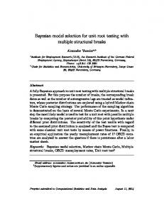
Table 2 Summary Statistics and Marginal and Stepwise Bayes Factors for Smoking and Pulmonary Health Data
Bi
r
B (r)
200
0.000
0
0.000
0.38
200
0.000
1
0.000
3.15
0.39
200
0.043
2
0.124
PS (2)
3.23
0.46
200
1.374
3
2.006
NI (1)
3.19
0.52
50
1.861
4
Stop
Group (#)
and
Mean
Std. Dev.
NS (0)
3.35
0.63
200
HS (5)
2.55
0.38
MS (4)
2.80
LS (3)
¯2 T¯r2 = n0 X 0 +
k X
n
k X
2
¯ j2 + 1 µ2 − ξ n0 X ¯0 + ¯ j + 1 µ /¯ nj X nj X nr /S 2 . ξ ξ j=r+1 j=r+1
Example 2. (White and Froeb 1980) The effect of smoking on pulmonary health is investigated in a retrospective study in which subjects who had been evaluated during a “physical fitness profile” were assigned, based on their smoking habits, to one of six groups – non-smokers (NS), passive smokers (PS), non-inhaling smokers (NI), light smokers (LS), moderate smokers (MS), and heavy smokers (HS). A sample of 1050 female subjects, 50 from non-inhaling group and 200 from each of the remaining groups, were selected and data on their pulmonary function (forced vital capacity, FVC) were recorded. One of the objectives of the study is to determine smoking effects on individual’s pulmonary health relative to non-smokers. With prior mean µ = 3 and ξ = 2, our Bayesian stepwise procedure stops at r = 3, rejects H5 , H4 and H3 and concludes that heavy, moderate, and light smokers are significantly different from non-smokers in terms of mean FVC (Table 2). An application of Dunnett’s two-sided method to the data suggests the same conclusion. 4.3. Multiple testing with an unknown control using one-sided hypotheses. We continue our discussion using the same distributional setups in the previous section, 17
but now we are interested in testing Hi : θi ≤ θ0
versus H i : θi > θ0 , i =
1, · · · , k, with θ0 being the unknown mean of the control group. Note that there is no discrete part of the prior distribution π1 (θi |ξ, σ 2 ). To avoid technical difficulty when calculating prior probability of Hi , we will use IG(σ 2 ; a/2, b/2) (instead of noninformative prior) as the prior density function of σ 2 and g(ξ) as the prior ¯ i is given density of ξ. It can be shown that the marginal Bayes factor for Hi over H by (1 − πi0 ) πi0 R Qk R − 12 −α R IG(σ 2 ; α, β) φ(z0 )Φ(zi0 )dz0 dσ 2 g(ξ)dξ j=0 nj β ·R Q , R − 12 −α R k IG(σ 2 ; α, β) φ(z0 ) [1 − Φ(zi0 )] dz0 dσ 2 g(ξ)dξ j=0 nj β R where πi0 = φ(z0 )Φ(z0 )dz0 is the prior probability of Hi , Φ and φ are, respectively,
(4.19)
Bi =
the cumulative distribution and density functions of standard normal, k 2 X n+a b S 1+ T 2j + 2 , α= , β= 2 2 S j=0 r z0 = and
n0 ξ
µ ¯0 + µ ¶ n0 ξ X θ0 − /σ, n0
1 z0 σ q ni + ξ n +
r zi0 =
0
1 ξ
¯ 0 + µ ni ξ X ¯i + µ n0 ξ X + − n0 ni
(See the Appendix for a proof.) The posterior probability of H (r) given X is Z Y Z n k (2π)− 2 Γ(α)(b/2)a/2 − 21 −α (r) (4.20) P (H |X) = nj β IG(σ 2 ; α, β) m∗0 (X)Γ(a/2) j=0 Z
·Y ¸ r k ¡ ¢ Y φ(z0 ) 1 − Φ(zj0 ) Φ(zj0 ) dz0 dσ 2 g(ξ)dξ j=1
j=r+1
(See the Appendix for a proof.) Per the recommendation of Berger, Boukai, and Wang (1997b), the prior g(ξ) is chosen to be an inverse gamma µ ¶ 1 1 (4.21) . g(ξ) = √ ξ −3/2 exp − 2ξ 2π The computation of the marginal Bayes factor for Hi and the posterior probability for H (r) is carried out using the method of Monte Carlo integration. 18
Table 3 Summary Statistics and Marginal and Stepwise Bayes Factors for Mouse Growth Data
Bi
r
B (r)
4
0.028
0
0.001
7.81
4
0.036
1
0.025
80.48
12.68
4
0.070
2
0.241
5
84.68
18.35
4
0.108
3
0.816
4
91.88
9.44
4
0.220
4
1.484
1
95.90
23.89
4
0.324
5
Stop
Group
Mean
Std. Dev.
n
0
105.38
13.44
4
3
72.14
8.41
6
74.24
2
Example 3. (Steel and Torrie 1980) The toxicological effects of six different chemical solutions on young mice are studied and compared with a control group in terms of weight change. The interest focuses on the comparisons of the six solutions with the control and not on the comparisons among the six solutions. Since it is generally believed that drugs are potentially toxic, it is appropriate to test the null hypotheses of no mean difference in weight gain against the one-sided alternative hypotheses of a lower weight gain. An application of Dunnett’s one-sided step-down method to the data reveals that solutions 3, 6, and 2 are significantly different from the control (Westfall, Tobias, Rom, Wolfinger, and Hochberg 1999, pp. 161-162). Using our proposed procedure with prior mean µ = 85 and a = b = 1, we conclude that solutions 3, 6, 2, and 5 are significantly more toxic than the control (Table 3).
5. Concluding remarks.
While there exist Bayesian methodologies to ad-
dress multiple testing problems, they either become too complicated to implement for large number of hypotheses or do not fully utilize the information that become available in the process of simultaneous testing of the hypotheses. Our idea of giving Bayesian formulations of the classical stepwise procedures is an attempt to overcome these shortcomings. Although we have decided in this article to propose a Bayesian version of the classical step-down method, we could have chosen the 19
classical step-up method and given its Bayesian version. In this step-up Bayesian method, once the target families were formed, the stepwise search would start from the family with no true null hypotheses and proceed towards those with higher number of true null hypotheses. Some recent papers (Efron 2003; Efron, Tibshirani, Storey, and Tusher 2001; Storey 2002; Storey 2003) have looked at multiple testing problems using a Bayesian formulation. More specifically, let Xi be the test statistics and Zi be Bernoulli random variables with the value 0 indicating that Hi is true and 1 indicating that it is false. They assume that Xi | Zi ∼ (1 − Zi )fi0 (x) + Zi fi1 (x) and P {Zi = 0} = πi0 , for i = 1, . . . , n. However, they provide Bayesian justifications of the frequentist measures of false discovery and positive false discovery rates. The idea of this article is completely different; we develop a stepwise decision procedure using Bayesian measures of evidence of different competing hypotheses. 6. Acknowledgments. The authors thank Larry Ma, Hong Qi, and Alice Cheng for helpful hints on SASr macros for computation of the examples.
20
APPENDIX A. APPENDIX A.1.
Proofs. Proof of (4.16).
By (3.5), the posterior probability of Hi : θi =
θ0 given X can be written as ½ ¾ ¡ ¢− ni ¤ 1 £ ¯ i − θ0 )2 + Si2 πi0 2πσ 2 2 exp − 2 ni (X 2σ
Z P (Hi |X) ∝
Y(−i) ½
Z
k
(2πσ 2 )−
(1 − πj0 )
nj +1 2
1
ξ− 2
j=1
¶¸ · µ 1 ¯ j − θj )2 + 1 (θj − µ)2 + Sj2 dθj exp − 2 nj (X 2σ ξ · ¸¾ nj ¢ 1 ¡ 2 − 2 2 2 ¯ +πj0 (2πσ ) exp − 2 nj (Xj − θ0 ) + Sj (σ 2 )−1 dσ 2 2σ Z k k Y X n n 1 ¯ j − θ0 )2 + S 2 πj0 (2π)− 2 (σ 2 )− 2 −1 exp − 2 nj (X = 2σ j=1 j=1 k
Y(−i) j=1
(
" Ã ¯ j − µ)2 1 − πj0 1 nj (X p 1+ exp − 2 2σ nj ξ + 1 πj0 nj ξ + 1 !#) ¯ j − θ0 )2 dσ 2 . −nj (X
To simplify the proof, let ¯ j − θ0 )2 , d¯j = nj (X
and
dj =
¯ j − µ)2 nj (X , nj ξ + 1
j = 1, . . . , k.
Notice that the expansion of the polynomial k
Y(−i) j=1
(1 + αj ) = 1 +
X(−i)
X(−i)
αj +
1≤j≤k
1≤j1 θ0 ·
dθ0 dσ 2 g(ξ)dξ =
n+k+1 (b/2)a/2 (2π)− 2 ∗ m0 (X)Γ(a/2)
·
1 exp − 2 2σ r Z Y
j=1
(A.32)
µX k
exp
exp
(σ 2 )−
n+a 2 −1
j=0
¶ 1 2 − 2 zj dzj 2σ
µ zj >zj0
Z 1
(nj ξ + 1)− 2
¶¸ Z µ ¶ ¯ j − µ)2 nj (X 1 2 2 +S +b exp − 2 z0 nj ξ + 1 2σ
µ
zj ≤zj0
Z k Y j=r+1
j=0
Z Y k
¶ 1 2 − 2 zj dzj dθ0 dσ 2 g(ξ)dξ 2σ
which simplifies to (4.21).
References Benjamini, Y. and Hochberg, Y. (1995). Controlling the false discovery rate: A practical and powerful approach to multiple testing. Journal of the Royal Statistical Society, Series B 57, 289–300. Berger, J. O. (1985). Statistical Decision Theory and Bayesian Analysis (2nd ed.). New York: Springer-Verlag. 28
Berger, J. O. (1999). Bayes factors. In S. Kotz, C. B. Read, and D. L. Banks (Eds.), Encyclopedia of Statistical Sciences, Volume 3, pp. 20–29. New York: Wiley. Berger, J. O., Boukai, B., and Wang, Y. (1997a). Properties of unified bayesianfrequentist tests. In S. Panchapakesan and N. Balakrishnan (Eds.), Advances in Statistical Decision Theory and Applications, pp. 207–224. Boston: Birkhauser. Berger, J. O., Boukai, B., and Wang, Y. (1997b). Unified frequentist and bayesian testing of a precise hypothesis. Statistical Science 12, 133–160. Berger, J. O., Boukai, B., and Wang, Y. (1999). Simultaneous bayesianfrequentist sequential testing of nested hypotheses. Biometrika 86, 79–92. Berger, J. O., Brown, L. D., and Wolpert, R. L. (1994). A unified conditional frequentist and Bayesian test for fixed and sequential simple hypothesis testing. The Annals of Statistics 22, 1787–1807. Berger, J. O. and Pericchi, L. R. (1996). The intrinsic Bayes factor for model selection and prediction. Journal of the American Statistical Association 91, 109–122. Berger, J. O. and Pericchi, L. R. (2001). Objective bayesian methods for model selection: Introduction and comparison. In P. Lahiri (Ed.), Model Selection. Beachwood, Ohio: Institute of Methematical Statistics Lecture Notes - Monograph Series, Volume 38. Berry, D. A. (1988). Multiple comparisons, multiple tests, and data dredging: A Bayesian perspective. In J. M. Bernardo, M. H. Degroot, D. V. Lindley, and A. F. M. Smith (Eds.), Bayesian Statistics 3, pp. 79–94. Berry, D. A. and Hochberg, Y. (1999). Bayesian perspectives on multiple comparisons. Journal of Statistical Planning and Inference 82, 215–227. Bertolino, F., Piccinato, L., and Racugno, W. (1995). Multiple Bayes factors for testing hypotheses. Journal of the American Statistical Association 90, 213–219. 29
Breslow, N. (1990). Biostatistics and bayes. Statistical Science 5, 269–298. Chen, J. and Sarkar, S. K. (2002). Multiple testing of response rates with a control: A Bayesian stepwise approach. submitted . Dass, S. and Berger, J. O. (1998). Unified Bayesian and conditional frequentist testing of composite hypotheses. Duke University: ISDS Discussion Paper 9843. Duncan, D. B. (1965). A Bayesian approach to multiple comparisons. Technometrics 7, 171–222. Dunnett, C. W. and Tamhane, A. C. (1991). Step-down multiple tests for comparing treatments with a control in unbalanced one-way layouts. Statistics in Medicine 11, 1057–1063. Dunnett, C. W. and Tamhane, A. C. (1992). A step-up multiple test procedure. Journal of the American Statistical Association 87, 162–170. Efron, B. (2003). Robbins, empirical Bayes and microarrays. Annals of Statistics 31, 366–378. Efron, B., Tibshirani, R., Storey, J. D., and Tusher, V. (2001). Empirical bayes analysis of a microarray experiment. Journal of the American Statistical Association 96, 1151–1160. Finner, H. (1993). On a monotonicity problem in step-down multiple test procedures. Journal of the American Statistical Association 88, 920–923. Gelman, A. and Tuerlinckx, F. (2000). Type S eerror rates for classical and Bayesian single and multiple comparison procedures. Computational Statistics [Formerly: Computational Statistics Quarterly] 15 (3), 373–390. Gopalan, R. and Berry, D. A. (1998). Bayesian multiple comparisons using dirichlet process priors. Journal of the American Statistical Association 93, 1130– 1139. Hochberg, Y. and Tamhane, A. C. (1987). Multiple Comparison Procedures. New York: John Wiley & Sons, Inc. 30
Holm, S. (1999). Multiple confidence sets based on stagewise tests. Journal of the American Statistical Association 94, 489–495. Hsu, J. C. (1996). Multiple Comparisons: Theory and Methods. Washinton, D.C.: Chapman & Hall/CRC. Liu, W. (1996). Multiple tests of a non-hierarchical finite family of hypotheses. Journal of the Royal Statistical Society, Series B 58, 455–461. Liu, W. (1997). Stepwise tests when the test statistics are independent. The Australian Journal of Statistics [Became: @J(AusNZJSt)] 39, 169–177. Romano, A. (1977). Applied Statistics for Science and Industry. Boston, MA: Allyn and Bacon. Sarkar, S. K. (2002). Some results on false discovery rate in stepwise multiple testing procedures. Annals of Statistics 30, 239–257. Shaffer, J. P. (1999). A semi-Bayesian study of Duncan’s Bayesian multiple comparison procedures. Journal of Statistical Planning and Inference 82, 197–213. Steel, R. G. D. and Torrie, J. H. (1980). Principles and Procedures of Statistics: A Biometrical Approach. New York: McGraw Hill Book Co. Storey, J. D. (2002). A direct approach to false discovery rates. Journal of the Royal Statistical Society, Series B 64, 479–498. Storey, J. D. (2003). The positive false discovery rate: A bayesian interpretation and the q-value. to appear in Annals of Statistics. Tamhane, A. C. and Dunnett, C. W. (1999). Stepwise multiple test procedures with biometric applications. Journal of Statistical Planning and Inference 82, 55–68. Tamhane, A. C. and Gopal, G. V. S. (1993). A Bayesian approach to comparing treatments with a control. In F. M. Hoppe (Ed.), Multiple Comparisons, Selection and Applications in Biometry. New York: Marcel Dekker, Inc. Tamhane, A. C., Liu, W., and Dunnett, C. W. (1998). A generalized step-updown multiple test procedure. The Canadian Journal of Statistics 26, 55–68. 31
Waller, R. A. and Duncan, D. B. (1969). A Bayes rule for the symmetric multiple compsrison problem. Journal of the American Statistical Association 64, 1484–1503. Westfall, P. H., Johnson, W. O., and Utts, J. M. (1997). A Bayesian perspective on the bonferroni adjustment. Biometrika 84, 419–427. Westfall, P. H. and Tobias, R. D. (1999). Advances in multiple comparisons and multiple tests using the SAS system. In Proceedings of the Twenty-Fourth Annual SAS Users Group International Conference, pp. 1525–1533. Cary, NC: SAS Institute, Inc. Westfall, P. H., Tobias, R. D., Rom, D., Wolfinger, R. D., and Hochberg, Y. (1999). Multiple Comparisons and Multiple Tests Using the SAS r System. Cary, NC: SAS Institute, Inc. Westfall, P. H. and Young, S. S. (1993). Resampling-Based Multiple Testing: Examples and Methods for p-Value Adjustment. New York: John Wiley & Sons. White, J. R. and Froeb, H. F. (1980). Small-airways dysfunction in nonsmokers chronically exposed to tobacco smoke. New England Journal of Medicine 302, 720–723.
Sanat K. Sarkar
Jie Chen
Department of Statistics
Merck Research Laboratories
Temple University
P. O. Box 4, WP37C-305
Philadelphia, PA 19122
West Point, PA 19486
U. S. A.
U. S. A.
E-mail:
[email protected]
E-mail: jie
[email protected]
32