A bi-level view of inpainting-based image compression

19th Computer Vision Winter Workshop Zuzana Kúkelová and Jan Heller (eds.) Kˇrtiny, Czech Republic, February 3–5, 2014

A bi-level view of inpainting - based image compression Yunjin Chen, René Ranftl, and Thomas Pock

arXiv:1401.4112v1 [cs.CV] 16 Jan 2014

Institute for Computer Graphics and Vision, Graz University of Technology, Austria {cheny,ranftl,pock}@icg.tugraz.at Abstract Inpainting based image compression approaches, especially linear and non-linear diffusion models, are an active research topic for lossy image compression. The major challenge in these compression models is to find a small set of descriptive supporting points, which allow for an accurate reconstruction of the original image. It turns out in practice that this is a challenging problem even for the simplest Laplacian interpolation model. In this paper, we revisit the Laplacian interpolation compression model and introduce two fast algorithms, namely successive preconditioning primal dual algorithm and the recently proposed iPiano algorithm, to solve this problem efficiently. Furthermore, we extend the Laplacian interpolation based compression model to a more general form, which is based on principles from bi-level optimization. We investigate two different variants of the Laplacian model, namely biharmonic interpolation and smoothed Total Variation regularization. Our numerical results show that significant improvements can be obtained from the biharmonic interpolation model, and it can recover an image with very high quality from only 5% pixels.

1

Introduction

Image compression is the task of storing image data in a compact form by reducing irrelevance and redundancy of the original image. Image compression methods roughly fall into two main types: lossless compression and lossy compression. In this paper, we focus on lossy compression methods. The objective of lossy compression methods is to reduce the original image data as much as possible while still providing a visually acceptable reconstruction from the compressed data. Lossy image compression can be handled with two different approaches: (1) reducing the data in the original image domain, i.e. by removing a majority of the image pixels; (2) reducing data in a transform domain, such as Discrete cosine transform (DCT) or Wavelet transform. The remaining data (compressed data) is used to reconstruct the original image. It is well known that the former approach is named as image inpainting in the literature [5, 2, 15], and the latter strategy is exploited in the currently widely used standard image compression techniques such as JPEG and JPEG2000 [12, 16]. In this paper, we focus on the strategy of reducing the data in the image domain and then recovering an image from a few data points, i.e., image inpainting.

There are thousands of publications studying the topic of image inpainting in the literature, see e.g., [5, 2, 15, 6] and references therein. In most cases, one does not have influence on the chosen data points. In the context of image inpainting, one usually randomly selects a specific amount of pixels which act as supporting points for the inpainting model, e.g., 5%. In order to get high quality reconstructions in such a scenario, one has to rely on sophisticated inpainting models. However, the task of image inpainting is to recover an image from only a few observations, and therefore, if the randomly selected data points do not carry sufficient information of the original image, even sophisticated inpainting models will fail to provide an accurate reconstruction. This observation motivated researchers to consider a different strategy for building inpainting based compression models, i.e. to find the optimal data points required for inpainting, given a specific inpainting model. Prior work in this direction can be found in [7, 10, 1, 14, 8, 9]. Belhachmi et al. [1] propose an analytic approach to choose optimal interpolation data for Laplacian interpolation, based on the modulus of the Laplacian. The work in [10] demonstrates that carefully selected data points can result in a significant improvement of the reconstruction quality based on the same Laplacian interpolation, when compared to the prior work [1]. However, this approach takes millions of iterations to converge and therefore is very time consuming. The very recent work [8] pushed forward this research topic, where the task of finding optimal data for Laplacian interpolation was explicitly formulated as an optimization problem, which was solved by a successive primal dual algorithm. While their work still requires thousands of iterations to reach a meaningful solution, this new model shed light on the possibility of employing optimization approaches and shows state-of-the-art performance for the problem of finding optimal data points for inpainting based image compression. The work of [8] is the starting point of this paper. In this paper, we extend the model of finding optimal data for Laplacian interpolation to a more general model, which comprises the model in [8] as a special case. We introduce two novel models to improve the compression performance, i.e., to get better reconstruction quality with the same amount of pixels. Finally, we introduce efficient algorithms to solve the corresponding optimization problems. Namely, we make the following two main contributions in this paper: (1) We comprehensively investigate two efficient algo-

A bi-level view of inpainting - based image compression rithms, which can be applied to solve the corresponding optimization problems, including successive preconditioning primal dual [13] and a recently published algorithm for nonconvex optimization - iPiano [11]. (2) We explore two variants of Laplacian interpolation based image compression to improve the compression performance, namely, a model based on the smoothed TV regularized inpainting model and biharmonic interpolation. It turns out that biharmonic interpolation can lead to significant improvements over Laplacian interpolation.

2

Extension of the Laplacian interpolation based image compression model

The original Laplacian interpolation is formulated as the following boundary value problem: −∆u = 0, on Ω \ I u = g, on I

(1)

∂n u = 0, on ∂Ω \∂I , where g is a smooth function on a bounded domain Ω ⊂ Rn with regular boundary ∂Ω. The subset I ⊂ Ω denotes the set with known observations and ∂n u denotes the gradient of u at the boundary. ∆ denotes the Laplacian operator. It is shown in [10, 8] that the problem (1) is equivalent to the following equation c(x)(u(x) − g(x)) − (1 − c(x))∆u(x) = 0, on Ω

(2)

∂n u(x) = 0, on ∂Ω \ ∂I , where c is the indicator function of the set I, i.e., c(x) = 1, if x ∈ I and c(x) = 0 elsewhere. By using the Neumann boundary condition, the discrete form of (2) is given by C(u − g) − (I − C)∆u = 0 ,

(3)

where the input image g and the reconstructed image u are vectorized to column vectors, i.e., g ∈ RN and u ∈ RN , C = diag(c) ∈ RN ×N is a diagonal matrix with the vector c on its main diagonal, ∆ ∈ RN ×N is the Laplacian operator and I is the identity matrix. The underlying philosophy behind this model is to inpaint the region (Ω \ I) by using the given data in region I, such that the recovered image is second-order smooth in the inpainting region, i.e., ∆u = 0. Note that the inpainting mask c in (3) is binary. However, as shown in [8], equation (3) still makes sense when c is relaxed to a continuous domain such as R. Due to this observation, the task of finding optimal interpolation data can be explicitly formulated as the following optimization problem: 1 min ku − gk22 + λkck1 u,c 2 s.t. C(u − g) − (I − C)∆u = 0 ,

(4)

where the parameter λ is used to control the percentage of pixels used for inpainting. When λ = 0, the optimal solution of (4) is c ≡ 1, i.e., all the pixels are used; when λ = ∞, the optimal solution is c ≡ 0, i.e., none of the pixel are used.

Figure 1: Linear operators shown as filters of size 5 × 5: from left to right, ∇x , ∇y , ∆ and biharmonic operator (∆2 )

Compared to the original formulation in [8], we omit a very small quadratic term 2ε kck22 , because we found that it is not necessary in practice. Observe that if c ∈ C = [0, 1)N , we can multiply the constraint equation in (4) by a diagonal positive-definite matrix (I − C)−1 , which results in B(c)(u − g) − ∆u = 0 ,

(5)

where B(c) = diag(c1 /(1 − c1 ), · · · , cN /(1 − cN )). It is clear that the constraint equation (5) can be equivalently formulated as the following minimization problem 1 1 1 (6) u(c) = arg min k∇uk22 + kB(c) 2 (u − g)k22 , u 2 2 where ∇ is the gradient operator, and ∆ = −∇> ∇. Therefore, it turns out that the Laplacian interpolation is exactly the Tikhonov regularization technique for image inpainting, where the first term can be seen as the regularization term based on the gradient operator, and the second term as the data fidelity term. Now, let us consider how to improve the performance of the regularization based inpainting model (6). The only thing we can change is the regularization term. There are two possible directions: (1) considering higher-order linear operators, e.g., ∆, to replace the first-order derivative operator ∇; (2) replacing the quadratic regularization with more robust penalty functions, such as `p quasi-norm with p ∈ (0, 1]. The linear operators ∇ and ∆ can be interpreted as linear filters, the corresponding linear filters are shown in Figure 1. If we make use of ∇ in the inpainting model (6), the resulting operator ∆ makes the inpainting process only involve the information from its nearest neighborhood; however, if we turn to the ∆ operator, the resulting operator ∆2 (biharmonic operator) can involve more information from larger neighborhood, see Figure 1. In principle, this should bring some improvement of inpainting performance; besides this, the biharmonic operator is mathematically meaningful in itself, implying higher-order smoothness of the solution u. Regarding the penalty function, quadratic function is known to generate over smooth results, especially for edges, and therefore many other edge-aware penalty functions have been proposed. A straightforward extension is to make use of the `1 norm, which leads to the well-known Total Variation (TV) regularization (still convex model). Since exact TV regularization suffers from the drawback of piece-wise constant solutions, we employ the following smoothed version of TV regularization, which is parameterized by a small smoothing parameter ε: N q X k∇ukε = (∇x u)2i + (∇y u)2i + ε2 , i=1

Yunjin Chen, René Ranftl, and Thomas Pock where ∇x u and ∇y u denote the gradient in x direction and y direction, respectively. We will show in the next section that this smooth technique is also necessary for optimization. Using these considerations, we arrive at a general formulation of the inpainting-based image compression model, which is given by the following bi-level optimization problem: 1 min ku(c) − gk22 + λkck1 (7) c∈C 2 1 1 s.t. u(c) = arg min R(u) + kB(c) 2 (u − g)k22 , u 2 where the upper level problem is defined as the trade-off between the sparsity of the chosen data and the reconstruction quality, while the lower-level problem is given as the regularization based inpainting model. In the lower-level problem, R(u) defines a regularization on u, and in this paper we investigate three different regularizers  1 2   2 k∇uk2 Laplacian interpolation 1 (8) R(u) = 2 k∆uk22 Biharmonic interpolation   k∇ukε Smoothed TV regularization

3

Efficient algorithms for solving inpainting based image compression problems

> ∂T > where Du = ∂T , D = , q = −Du u ˆ− c ∂u u ∂c ˆ cˆ Dc cˆ. Note that the linearized constraint is only valid around a small neighborhood of (ˆ u, cˆ), and therefore we have to add ˆk22 to two additional penalty term µ21 kc − cˆk22 and µ22 ku − u ∗ ∗ ensure that the solution (u , c ) is in the vicinity of (ˆ u, cˆ). The saddle-point formulation of (11) is written as u 1 max min K + q, p + ku − gk22 + λkck1 + p (u,c) c 2 µ2 µ1 2 kc − cˆk2 + ku − u ˆk22 + δC (c) , (12) 2 2 where K = (Du , Dc ), δC (c) is the indicator function of set C, and p ∈ RN is the Lagrange multiplier associated with the equality constraint in (11). Remark 1. Note that for Laplacian and biharmonic interpolation, we do not restrict c to the set C, and we make use of the original constraint in (4), i.e., C(u − g) − (I − C)Lu = 0 , where L = −∆ for Laplacian interpolation, and L = −∆2 for biharmonic interpolation. Therefore, the indicator function δC (c) in equation (12) can be dropped for these models. However, for the TV regularized model or other possible regularization techniques, we have to strictly rely on (12).

In the prior work [8], a successive primal dual algorithm was used in order to solve the Laplacian interpolation based image compression problem (7), where tens of thousands inner iterations and thousands of outer iterations are required to reach convergence. Since this is too time consuming for practical applications, we first investigate efficient algorithms to solve problem (7).

Remark 2. It was stated in previous work [8] that there is no need to introduce an additional penalty term for variable u, because u continuously depends on c. However, we find that for biharmonic interpolation, we have to keep the penalty term for u, otherwise, the resulting algorithm will suffer from zigzag behavior when it gets close to the optimal solution.

3.1

It is easy to work out the Jacobi matrices Du and Dc for Laplacian and biharmonic interpolation, which are given as ( Du (ˆ u, cˆ) = diag(ˆ c) − (I − diag(ˆ c))L, Dc (ˆ u, cˆ) = diag(ˆ u − g + Lˆ u) .

Successive Preconditioning Primal Dual algorithm (SPPD)

A straightforward method to accelerate the algorithm in [8] is to make use of the diagonal preconditioning technique [13] for the inner primal dual algorithm, while keeping the outer iterate unchanged. The basic principle of the successive primal dual algorithm, is to linearize the constraint of (7), i.e., the lower-level problem. For smooth regularization terms R(u), the lower-level problem of (7) can be equivalently written using its first-order optimality conditions: ∂R(u) T (u, c) = + B(c)(u − g) = 0. (9) ∂u Using Taylor expansion, we linearize (9) around a point (ˆ u, cˆ): > > ∂T ∂T (u−ˆ u)+ (c−ˆ c) = 0. T (u, c) ≈ T (ˆ u, cˆ)+ ∂u uˆ ∂c cˆ (10) Let (ˆ u, cˆ) be a feasible point of constraint (9), i.e., T (ˆ u, cˆ) = 0, and substitute the linearized constraint back into the initial problem (7), we arrive at the following constrained optimization problem µ1 µ2 1 min ku − gk22 + λkck1 + kc − cˆk22 + ku − u ˆk22 c∈C,u 2 2 2 s.t. Du u + Dc c + q = 0 , (11)

For smooth TV regularized inpainting model, the constraint (9) is written as ∇x u > ∇ · ∇ρ u + B(u − g) = 0 , x

ρ

q x where ρ = ∇2x u + ∇2y u + ε2 , and ∇ = ∇ ∇y . The Jacobi matrices Du and Dc are given by  1 u, cˆ) = diag( (1−c)  2 ) · diag(u − g), Dc (ˆ  2  ∇2 y u+ε  ∇x  > ρ3 x Du (ˆ u, cˆ) = ∇ · diag · ∇y − 2 ∇2 u+ε ∇y x ρ3   ∇x u ∇y u  ∇x  ∇y > ρ3   · ∇y + B , · diag ∇ x u ∇y u ∇x ρ3

(13) where denotes point-wise multiplication. We make use of the diagonal preconditioning technique of [13] to choose the preconditioning matrices Γ and Σ. Γ = diag(τ ), Σ = diag(σ) ,

A bi-level view of inpainting - based image compression Algorithm 3.1 Preconditioning PD for solving problem (12) (1) Compute the preconditioning matrices Γ and Σ and choose θ ∈ [0, 1]

where A = C + (C − I)L. Casting (16) in the form of iPiano algorithm, we have F (c) = 21 kA−1 diag(c)u − gk22 , and G(c) = λkck1 . As shown in [11], the gradient of F with respect to c is given as:

(2) Initialize (u, c) with (ˆ u, cˆ), and p¯ = 0.

∇F (c) = diag(−(I + L)u + g)(A> )−1 (u − g) .

(3) Then for k ≥ 0, update (uk , ck ) and pk as follows:  uk k+1 k  p = p + Σ K + q k  c 

k p¯k+1 = pk+1 + θ(pk+1 − p k)  k+1   u = (I + Γ∂G)−1 u − ΓK > p¯k+1 ck+1

ck

(14)

1 PN 2−γ , σi i=1 |Ki,j |

P2N 1 γ . j=1 |Ki,j |

= The we emwhere τj = ploy the preconditioning primal dual Algorithm 3.1 to solve problem (12). For Laplacian and biharmonic interpolation, the function G(u, c) in (14) is given as µ2 µ1 1 ku − gk22 + ku − u ˆk22 + λkck1 + kc − cˆk22 . 2 2 2 It turns out that the proximal map with respect to G simply poses point-wise operations, which is given as ˜ u −1 u = (I + Γ∂G) ⇐⇒ c˜ c  u ˜ +τi1 gi +µ2 τi1 u î  i = 1···N ui = i 1+τ 1 1 i +µ2 τi (15) c˜i +τi2 µ1 cî ,  1+τi2 µ1 ci = shrink λτ2i2

For smooth TV regularization, F (c) = 12 ku(c) − gk22 , u(c) is the solution of the lower-level TV regularized inpainting model. In order to calculate the gradient of F with respect to c, we can make use of the implicit differentiation technique, see [3] for more details. The gradient is given as ∇F (c) c∗ = −Dc (u∗ , c∗ )(Du (u∗ , c∗ ))−1 (u∗ − g) , where u∗ is the optimal solution of the lower-level problem in (7) at point c∗ . As stated in [3], in order to get an accurate gradient ∇F (c), we need to solve the lower-level problem as accurately as possible. To that end, we exploit Newton’s method to solve the lower-level problem. Now we can make use of iPiano to solve this optimization problem. The algorithm is summarized below:

G(u, c) =

1+τ µ1 i

where the soft shrinkage operator is given by shrinkα (x) = 1 sgn(x) · max(|x| − α, 0), and τ = ττ 2 . For smooth TV regularization, the function G is given by G(u, c) =

(1) Choose β ∈ [0, 1), l−1 > 0, η > 1, and initialize c0 = 1 and set c−1 = c0 . (2) Then for n ≥ 0, conduct a line search to find the smallest nonnegative integers i such that with ln = η i ln−1 , the following inequality is satisfied

F (cn+1 ) ≤ F (cn ) + ∇F (cn ), cn+1 − cn ln (17) + kcn+1 − cn k22 , 2 where cn+1 is calculated from (18) by setting β = 0. Set ln = η i ln−1 , αn < 2(1 − β)/ln , and compute

N X

1 µ2 µ1 ku−gk22 + ku−ˆ uk22 +λ ci + kc−ˆ ck22 +δC (c). 2 2 2 i=1

The proximal map for u is the same as in (15), the solution for c can be computed by c˜i + τi2 µ1 cî − τi2 λ ci = ProjC 1 + τi2 µ1 3.2

Algorithm 3.2 iPiano for solving problem (12)

iPiano

Observe that in problem (7) the lower-level problem can be solved for u, and the result can be substituted back into the upper-level problem. It turns out that this results in an optimization problem which only depends on the variable c. It is demonstrated in our previous work [11] that this optimization problem can be solved efficiently by using the recently proposed algorithm - iPiano. Our experiments will show that this strategy is more efficient than the successive preconditioning primal dual algorithm. For Laplacian and biharmonic interpolation, we can solve u in closed form, i.e., u = A−1 Cg. This results in the following optimization problem, which only depends on variable c: 1 (16) min kA−1 diag(c)g − gk22 + λkck1 , c 2

cn+1 = (I +αn ∂G)−1 (cn −αn ∇F (cn )+β(cn −cn−1 )) . (18)

4

Numerical experiments

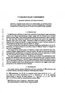
In this section, we first discuss how to choose an efficient algorithm for solving the model (7) for different cases. Then we investigate the inpainting performance for different models under the unified assumption that we only make use of 5% pixels. All the experiments were conducted on a server with Intel X5675 processors (3.07GHz), and all the investigated algorithms were implemented in pure Matlab code. We exploited three different test images (“Trui”, “Walter” and “Peppers”) which are also used in previous works [10, 8]. 4.1

Implementation details

In our implementation, the parameter γ of preconditioning technique is chosen as γ = 10−6 . For the SPPD algorithm, the parameter µ1 and µ2 are set as follows: (1) for the Laplacian interpolation based compression model, µ1 =

Yunjin Chen, René Ranftl, and Thomas Pock

(a) Trui

(b) Peppers

(c) Walter

(d) Lena

Figure 2: Four test images used in our experiments

0.05, µ2 = 0; (2) for biharmonic interpolation based model, µ1 = 0.1, µ2 = 0.2; and (3) for smoothed TV based model, µ1 = 0.05, µ2 = 0.1. The set C is defined in the range of [0, cmax ] with cmax = 1 − 10−6 . For the iPiano algorithm, we make use of the following parameter settings: l−1 = 1, η = 1.2, β = 0.75, αn = 1.99(1 − β)/ln . In order to exploit possible larger step size in practice, we use the following heuristic: If the line search inequality (17) is fulfilled, we decrease the evaluated Lipschitz constant Ln slightly by using a factor 1.02, i.e., setting ln = ln /1.02. 4.2

Choosing appropriate algorithm for each individual model

For Laplacian interpolation based compression model, we found that when using the proposed preconditioning technique, the required iterations can be reduced to about 150 outer iterations and 2000 inner iterations, which is a tremendous decrease compared to prior work [8]. However, for this problem, the iPiano algorithm can do better. Our experiments show that usually 700 iterations are already enough to reach a lower energy. Concerning the run time, the SPPD algorithm needs about 2400s, but iPiano only takes about 622s. We conclude that iPiano is clearly a better choice for solving the Laplacian interpolation based compression model. Let us turn to the biharmonic interpolation based compression model. Even though the linear operator is only slightly changed, when compared to the Laplacian model, it turns out that the corresponding optimization problem becomes much harder to solve. The SPPD algorithm still works for this problem; however, as mentioned before, we have to introduce an additional penalty term on variable u, otherwise the convergence behavior is very bad. Besides, we have to run the algorithm much longer, usually about 300 outer iterations and 4000 inner iterations. For the iPiano algorithm applied to this case, we have to significantly increase the amount of required iterations, typically, we have to run about 3500 iterations to reach convergence. For the biharmonic interpolation based compression model (16), the difference between the results obtained by above two algorithms becomes more obvious. For instance, for the test image “Trui” with parameter λ = 0.0028,

by using the SPPD algorithm, we arrive a final energy of 15.34; however, the final energy of iPiano is much lower, about 13.48, which basically implies that iPiano solves the corresponding optimization problem better. Concerning the run time, for this case, iPiano takes more computation time than Laplacian interpolation case. There are two reasons: (1) the amount of required iterations is increased by a factor of 5; (2) for iPiano, we have to solve two linear equation Ax = b and A> x = b in each iteration and line search1 , which becomes much more time consuming from Laplacian to biharmonic interpolation. Therefore, for this case, both algorithms show a similar runtime (about 5000s). Since iPiano achieves a lower energy with similar computational effort this algorithm is preferable for the biharmonic model. For the case of smoothed TV regularization, it becomes even harder to solve the lower-level problem and thus more time consuming. It is therefore advisable not to make use of iPiano. The SPPD algorithm is a better choice for this model. Solving smoothed TV regularization based model also needs about 5000s. 4.3

Reconstruct an image only using ∼5% pixels

We evaluate the performance of three considered compression models based on three test images. For each individual model, we search optimal data points used for inpainting with the same amount of about 5%, and then reconstruct an image by using these optimal points. In order to control the sparsity of selected data points to be 5% approximately, we have to carefully choose the parameter λ for each model and for each processing image. The found optimal mask c is continuous, and then we binarize it by a threshold parameter εT = 0.01. Concerning the measurement of reconstruction quality, we make use of the mean squared error (MSE) to keep consistent with previous work, which is given by M SE(u, g) =

N 1 X (ui − gi )2 . N i=1

The MSE is computed with the assumption that the image gray value is in the range of [0, 255]. As shown in previous work [8], for Laplacian interpolation, it is straightforward to consider an additional post-processing step, which is called 1 In

our implementation we use the Matlab “backslash” operator.

A bi-level view of inpainting - based image compression

(a) 10% random chosen data

(b) Smoothed TV (276.37)

(c) Laplacian (244.48)

(d) Biharmonic (208.92)

(e) Learned prior (165.01)

Figure 3: Inpainting results of the degraded “Lena” image with 10% randomly chosen pixels by using different methods. The number in the bracket is the resulting MSE. For randomly selected points, the inpainting model with learned MRF prior gives the best reconstruction result.

gray value optimization (GVO) to further improve the reconstruction quality. We also consider this strategy for Laplacian and biharmonic interpolation after binarising the mask c, which is formulated as following optimization problem arg min kA−1 S > x − gk22 , x∈RM

(19)

where A is defined in the same way as in (16). S ∈ RM ×N is the sampling matrix derived from the diagonal matrix diag(c) by deleting the rows whose elements are all zero. M is the number of points in the mask c with a value of 1. Obviously, (19) is a least squared problem, which has the closed form solution −1 x = S(A> )−1 A−1 S > S(A> )−1 g. However, in practice it turns out that this computation is very time consuming because we have to calculate A−1 explicitly. Therefore, we turn to L-BFGS algorithm to solve this quadratic optimization problem. For smoothed TV regularization model, we also consider this GVO post-processing step, which is given by the following bi-level optimization problem 1 (20) min l(x) = ku(x) − gk22 2 x∈RM 1 1 s.t. u(x) = arg min k∇ukε + kB 2 (u − S > x)k22 , u 2 where the sampling matrix S ∈ RM ×N is the same as in (19). We also make use of L-BFGS to solve this problem. To that end, we need to calculate the gradient of l with respect to x, which is given as ∇l(x) ∗ = −Dx (u∗ , x∗ )(Du (u∗ , x∗ ))−1 (u∗ − g) , x

where Du is the Hessian matrix given in (13), Dx = −SB, u∗ is the solution of the lower-level problem at point x∗ . We summarize the results in Figure 4. One can see that starting from the initial Laplacian interpolation based image compression model, we can achieve significant improvements of inpainting performance for all test images by using biharmonic interpolation based model, at the expense of computation time; however, switching to the smoothed TV regularization based model can not bring any improvement even with more computation time. To the best of our knowledge, concerning the inpainting performance of the biharmonic interpolation model, it is the first time to achieve such an accurate reconstruction by using only 5% pixels.

5

Conclusion and future work

In this paper, we extended the Laplacian interpolation based image compression model to more general inpainting based compression model. Starting from the Laplacian interpolation, we investigated two variants, namely biharmonic interpolation and smoothed TV regularization inpainting model, to improve the compression performance. In order to solve the corresponding optimization problems efficiently, we introduced two fast algorithms: (1) successive preconditioning primal dual algorithm and (2) a recently proposed nonconvex optimization algorithm - iPiano. Based on these algorithms, for each model, we found the most useful 5% pixels, and then reconstructed an image from the optimal data. Numerical results demonstrate that (1) biharmonic interpolation gives the best reconstruction performance and (2) the smoothed TV regularization model can not generate superior results over the Laplacian interpolation method. Future work consists of two aspects: (1) more efficient algorithm to solve the corresponding optimization problems. Even though the introduced algorithms are fast, they are still very time consuming for complicated models, e.g., biharmonic interpolation and smoothed TV regularization models. (2) exploiting more sophisticated inpainting models to further improve the compression model. A possible candidate is to make use of the inpainting model with a learned MRF prior [3, 4], which is shown to work well for image inpainting with randomly selected points. Figure 3 presents an example to show the inpainting performance of the learned model for randomly selected data points. One can see that in this random case, the inpainting model with learned MRF prior can generate the best result, and therefore, we believe that it can achieve better result for image compression.

References [1] Zakaria Belhachmi, Dorin Bucur, Bernhard Burgeth, and Joachim Weickert. How to choose interpolation data in images. SIAM Journal on Applied Mathematics, 70(1):333–352, 2009. [2] Marcelo Bertalmio, Guillermo Sapiro, Vincent Caselles, and Coloma Ballester. Image inpainting. In Proceedings of the 27th annual conference on Computer graphics and interactive techniques,

pages 417–424. ACM Press/Addison-Wesley Publishing Co., 2000.

Yunjin Chen, René Ranftl, and Thomas Pock [3] Y.J. Chen, T. Pock, R. Ranftl, and H. Bischof. Revisiting loss-specific training of filter-based MRFs for image restoration. In German Conference on Pattern Recognition (GCPR), 2013. [4] Y.J. Chen, R. Ranftl, and T. Pock. Insights into analysis operator learning: from patch-based models to higher-order MRFs. To appear in IEEE Transactions on Image Processing, 2014. [5] Antonio Criminisi, Patrick Pérez, and Kentaro Toyama. Region filling and object removal by exemplar-based image inpainting. Image Processing, IEEE Transactions on, 13(9):1200–1212, 2004. [6] Julia A Dobrosotskaya and Andrea L Bertozzi. A wavelet-laplace variational technique for image deconvolution and inpainting. Image Processing, IEEE Transactions on, 17(5):657–663, 2008. [7] I. Galic, J. Weickert, M. Welk, A. Bruhn, A. G. Belyaev, and H.-P. Seidel. Image compression with anisotropic diffusion. Journal of Mathematical Imaging and Vision, 31(2-3):255–269, 2008. [8] L. Hoeltgen, S. Setzer, and J. Weickert. An optimal control approach to find sparse data for Laplace interpolation. In International Conference on Energy Minimization Methods in Computer Vision and Pattern Recognition (EMMCVPR), pages 151–164, 2013.

[9] M. Mainberger, A. Bruhn, J. Weickert, and S. Forchhammer. Edge-based compression of cartoon-like images with homogeneous diffusion. Pattern Recognition, 44(9):1859–1873, 2011. [10] M. Mainberger, S. Hoffmann, J. Weickert, C. H. Tang, D. Johannsen, F. Neumann, and B. Doerr. Optimising spatial and tonal data for homogeneous diffusion inpainting. In International Conference on Scale Space and Variational Methods in Computer Vision (SSVM), pages 26–37, 2011. [11] Peter Ochs, Yunjin Chen, Thomas Brox, and Thomas Pock. ipiano: Inertial proximal algorithm for non-convex optimization. Preprint, 2013. [12] William B Pennebaker. JPEG: Still image data compression standard. Springer, 1992. [13] Thomas Pock and Antonin Chambolle. Diagonal preconditioning for first order primal-dual algorithms in convex optimization. In International Conference on Computer Vision (ICCV 2011), 2011. [14] C. Schmaltz, J. Weickert, and A. Bruhn. Beating the quality of JPEG 2000 with anisotropic diffusion. In DAGM-Symposium, pages 452–461, 2009. [15] Jianhong Shen. Inpainting and the fundamental problem of image processing. SIAM news, 36(5):1–4, 2003. [16] D Taubman and MW Marcellin. JPEG2000: Image compression fundamentals, practice and standards. Massachusetts: Kluwer Academic Publishers, pages 255–258, 2002.

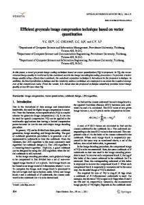
(a) 4.98%

(b) 4.98%

(c) 6.90%

(d) 4.95%

(e) MSE: 16.89

(f) MSE: 10.60

(g) MSE: 17.98

(h) MSE: 16.95

(i) 4.84%

(j) 4.89%

(k) 5.69%

(l) 5.02%

(m) MSE: 18.99

(n) MSE: 17.81

(o) MSE: 21.14

(p) MSE: 18.44

(q) 4.82%

(r) 4.59%

(s) 5.86%

(t) 5.00%

(u) MSE: 8.03

(v) MSE: 4.85

(w) MSE: 10.52

(x) MSE: 7.59

Figure 4: Image inpainting results by using approximate 5% pixels. The interpolation data points used for reconstruction is masked in black. The continuous mask c is binarized with a threshold parameter εT = 0.01. From left to right: (1) optimal mask found with Laplacian interpolation and the corresponding recovery image by using the optimal data points, (2) results of biharmonic interpolation model, (3) results of smoothed TV regularization approach, (4) results of [8]