A Boosting Algorithm for Learning Bipartite Ranking Functions with Partially Labeled Data Massih-Reza Amini, Tuong-Vinh Truong
Cyril Goutte
Université Pierre et Marie Curie Laboratoire d’Informatique de Paris 6 104, avenue du Président Kennedy 75016 Paris, France
National Research Council Canada Institute for Information Technology 283, boulevard Alexandre-Taché Gatineau, QC J8X 3X7, Canada
[email protected]
{amini,truong}@poleia.lip6.fr
ABSTRACT This paper presents a boosting based algorithm for learning a bipartite ranking function (BRF) with partially labeled data. Until now different attempts had been made to build a BRF in a transductive setting, in which the test points are given to the methods in advance as unlabeled data. The proposed approach is a semi-supervised inductive ranking algorithm which, as opposed to transductive algorithms, is able to infer an ordering on new examples that were not used for its training. We evaluate our approach using the TREC-9 Ohsumed and the Reuters-21578 data collections, comparing against two semi-supervised classification algorithms for ROCArea (AUC), uninterpolated average precision (AUP), mean precision@50 (mT9P) and Precision-Recall (PR) curves. In the most interesting cases where there are an unbalanced number of irrelevant examples over relevant ones, we show our method to produce statistically significant improvements with respect to these ranking measures.
Categories and Subject Descriptors H.3 [Information Storage and Retrieval]: Information Search and Retrieval - Information Routing; H.1 [Models and Principles]: Miscellaneous
General Terms Algorithms, Experimentation, Theory
Keywords Learning to Rank with partially labeled data, Boosting, Information Routing
1.
INTRODUCTION
Learning with partially labeled data or semi-supervised learning has been widely studied under the classification framework [5, 13, 16, 20, 3, 11, 8]. However, there are many
Permission to make digital or hard copies of all or part of this work for personal or classroom use is granted without fee provided that copies are not made or distributed for profit or commercial advantage and that copies bear this notice and the full citation on the first page. To copy otherwise, to republish, to post on servers or to redistribute to lists, requires prior specific permission and/or a fee. SIGIR’08, July 20–24, 2008, Singapore. Copyright 2008 ACM 978-1-60558-164-4/08/07 ...$5.00.
applications where the goal is to learn a ranking function and for which training sets are hard to obtain mainly because the labeling of examples is time consuming, and sometimes even unrealistic. This is for example the case for domain specific search engines or routing systems [18] where, for a stable user’s information need there is a stream of incoming documents which have to be dynamically retrieved. The constitution of a labeled training set is, in this case, a difficult task. But, if such a training set is available the goal of learning would be to find a bipartite ranking function (BRF) which assigns a higher score to relevant examples than to irrelevant ones1 . Recently some studies have addressed the use of unlabeled data to learn a BRF in a transductive setting [1, 22, 24, 23]. In this case, one is given sample points from a labeled training set and an unlabeled test set, and the goal is to build a prediction function which orders only unlabeled examples from the test set. This restriction makes the design of a ranking function that assigns scores to new examples inherently inconvenient. Neither can existing work on leveraging unlabeled data for classification of pairwise examples be applied directly to learn a BRF. As some pairs would have the same instances in common, this would violate the independence assumption on which classifier learning is based. In this paper we present a new inductive ranking algorithm which builds a prediction function on the basis of two labeled and unlabeled training sets: one labeled and one unlabeled. In a first stage, the algorithm loops over the labeled set and assigns, for each labeled training example, the same relevance judgment to the most similar examples from the unlabeled training set. An extended version of the RankBoost algorithm [10] is then developed to produce a scoring function that minimizes the average number of incorrectly ordered pairs of (relevant, irrelevant) examples, over the labeled training set and the tentatively labeled part of the unlabeled data. The novelty of the approach is that the algorithm optimizes an exponential upper bound of a learning criterion which combines the misordering loss for both parts of the training set. Experiments on the TREC-9 Ohsumed and Reuters-21578 datasets, show that the proposed approach is effective on AUC, AUP, mT9P and PR ranking measures especially when there are much less relevant examples than irrelevant ones. In addition, comparisons involving two semi-supervised clas1
These forms of ranking correspond to the bipartite feedback case studied in [10] and we hence refer to them as the bipartite ranking problems.
sification algorithms indicate that, as in the supervised case [7, 9], the error rate of a semi-supervised classification function is not necessarily a good indicator of the accuracy of the ranking function derived from it. In the remainder of the paper, we discuss, in section 2, the problem of semi-supervised learning for bipartite ranking. In sections 2.1 and 2.2, we present a boosting based algorithm to find such ranking functions. In section 4, we present experimental results obtained with our approach on the TREC-9 Ohsumed and the Reuters-21578 datasets. Finally, in section 5 we discuss the outcomes of this study and give some pointers to further research.
2. SEMI-SUPERVISED BIPARTITE RANKING In bipartite ranking problems such as information routing [17], examples from an instance space X ∈ Rd are assumed to be relevant or irrelevant to a given search profile or topic. The goal of learning can then be defined as the search of a scoring function H : X → R which assigns higher scores to relevant instances than to irrelevant ones [10]. In this setting, the system is usually given a sample of n labeled instances Zℓ = {xi , yi }i∈{1,...,n} where each example x ∈ Zℓ is associated with a relevance judgment yi ∈ {−1, 1}, representing the fact that xi is relevant (yi = +1) or not (yi = −1) to that topic. The learning task reduces to minimization of the average number of irrelevant instances in Zℓ scored better than relevant ones by H [10]. In the semisupervised setting, we further assume that together with labeled examples in Zℓ , we also have a set of m unlabeled examples XU = {x′i }i∈{n+1,...,n+m} and, we propose to learn a ranking function on the basis of these two training sets. In order to exploit information from XU , we assume that an unlabeled instance from XU that is similar to a labeled instance from Zℓ should have similar label. We begin by selecting examples in XU that are the most similar to a labeled example x ∈ Zℓ and assign them the corresponding relevance judgment y. At this stage, a simple approach would consist in adding these new examples from XU to the labeled training set and then learn a ranking function as in the usual supervised case. This training scheme suffers from a real drawback in that as unlabeled examples are given error-prone labels, the resulting ranking would be highly dependent on how robust the training scheme is to noisy labels. Therefore, instead of mixing Zℓ with selected examples in XU , we suggest minimizing the ranking errors on each training sets separately. Formally, let AC be an unsupervised algorithm which specifies, for each labeled data, the unlabeled instances that are the most similar to it. And, let ZU\ be the set of unlabeled examples obtained from AC that have been assigned labels according to similar labeled data. Our goal is thus to find a function H, which minimizes the average numbers of irrelevant examples scored better than relevant ones in Zℓ and ZU\ separately. We call this quantity the average ranking ˆ n+m , defined as: loss, R ˆ n+m (H, Zℓ ∪ ZU\ ) = R +
1 PZℓ λ PZ′ U\
Where, X+ and X− (resp.) represent the sets of relevant and irrelevant (resp.) instances in Zℓ , while X+′ = AC (X+ ) and X−′ = AC (X− ) (resp.) are the sets of unlabeled data which are similar to relevant and irrelevant (resp.) instances in Zℓ . PZℓ = |X− ||X+ | and PZ′ U\ = |X−′ ||X+′ | (resp.) are the number of relevant and irrelevant pairs in Zℓ and ZU\ (resp.). (x+ , x− ) and (x′+ , x′− ) (resp.) denote pairs of (relevant, irrelevant) examples in X+ ×X− and X+′ ×X−′ (resp.). Finally, λ is a discount factor2 and [[π]] is equal to 1 if the predicate π holds and 0 otherwise. Several successful Machine Learning algorithms, including various versions of boosting and support vector machines are based on replacing the loss function by a convex function [4]. This approach has important computational advantages, as the minimization of the empirical convex functional is feasible by, for example, gradient descent algorithms. In the following we extend the majoration of the supervised ranking loss proposed by [10] to the semi-supervised bipartite ranking case. Using the upper bound [[x ≥ 0]] ≤ ex , we get the following exponential loss: En+m (H) =
1 X H(x− )−H(x+ ) λ X H(x′− )−H(x′+ ) e e + ′ PZℓ x ,x PZU\ ′ ′ +
−
x+ ,x−
As for the meta-search task [21] and Pfollowing [10], we define the final ranking function, H = t αt ft , as a weighted sum of the ranking features ft . Each ranking feature ft is uniquely defined by an input feature jt ∈ {1, ..., d} and a threshold θt : 1, if ϕjt (x) > θt ft (x) = (1) 0, else where, ϕj (x) is the j th feature characteristic of x. The learning task is then defined as the search of the combination weights αt and the ranking features ft for which the minimum of the exponential loss En+m (H) is reached.
2.1 A Boosting based Algorithm Derivation The ranking problem presented in the previous section can be implemented efficiently by extending the RankBoost algorithm proposed in [10]. This extension iteratively main˜ t over pairs of (relevant, tains two distributions Dt and D irrelevant) examples in Zℓ and ZU\ . At the beginning, all pairs are supposed to be uniformly distributed, that is, ∀(x− , x+ ) ∈ X− × X+ , D1 (x− , x+ ) = ′ ′ 1 ˜ 1 (x′− , x′+ ) = ′1 . At and ∀(x′− , x′+ ) ∈ X− × X+ ,D PZ P ℓ
ZU \
˜ t are then gradually updated in order each round, Dt and D to give increasing weights to pairs that are difficult to rank correctly. The weight for each pair is therefore increased or decreased depending on whether ft orders that pair incorrectly, leading to the update rules: Dt+1 (x− , x+ ) =
Dt (x− , x+ ) exp(αt (ft (x− ) − ft (x+ ))) (2) Zt
and X
[[H(x− ) ≥ H(x+ )]]
X
[[H(x′− ) ≥ H(x′+ )]]
x+ ,x− ∈X+ ×X−
′ ×X ′ x′+ ,x′− ∈X+ −
′ ′ ˜ ′ ′ ˜ t+1 (x′− , x′+ ) = Dt (x− , x+ ) exp(αt (ft (x− ) − ft (x+ ))) (3) D Z˜t 2 For λ = 0, we fall back to the situation of standard supervised learning.
where Zt =
X
Dt (x− , x+ )eαt (ft (x− )−ft (x+ )) and Z˜t =
x− ,x+
X
′
′
Dt (x′− , x′+ )eαt (ft (x− )−ft (x+ )) are normalization factors
x′− ,x′+
˜ t+1 remain probability distributions. such that Dt+1 and D The search of the ranking feature ft and its associated weight αt are carried out by directly minimizing the exponential loss, En+m . This optimization is performed first by noticing that the exponential loss En+m writes: En+m (H) =
T Y
Zt + λ
t=1
T Y
Z˜t ,
(4)
t=1
Algorithm 1: Learning BRF with partially labeled data Given : • Zℓ = X+ ∪ X− , a labeled training set and ′ ′ ZU\ = X+ ∪ X− , a labeled subset of XU obtained from AC , • Set ν1 (x) = |X1+ | if x ∈ X+ and ν1 (x) = |X1− | if x ∈ X− , ′ • Set ν˜1 (x′ ) = |X1′ | if x′ ∈ X+ and ν˜1 (x′ ) = |X1′ | if
for t := 1, ..., T do • Train a ranking feature ft : X → R using νt and ν˜t
where, T is the maximum number of rounds. This rewriting results from the update rules (2-3), the use of a linear ranker PT H = t=1 αt ft , the exponential homomorphism property ˜ t sum to one for ex+y = ex ey and the fact that Dt and D every t. The selection of ranking features is presented in section 2.2. The choice of the weight combinations, αt , results from the minimization of (4). At each iteration, this minimization is performed by rewriting the exponential loss as En+m (H) = At−1 Zt + λBt−1 Z˜t , where, At−1 =
t−1 Y
Zk and Bt−1 =
t−1 Y
• Choose the weight αt , as defined by equation (6) • Update νt+1 (x) =
νt (x) exp(−αt ft (x)) if x ∈ X+ Zt+ νt (x) exp(αt ft (x)) if x ∈ X− Zt−
where Zt+ and Zt− normalize νt over X+ and X− • Update
(5)
′
ν˜t+1 (x ) =
Z˜k . Eq. 5 can then
be upper-bounded by the following expression: »„ « « „ – 1 − rt 1 + rt En+m (H) ≤ At−1 eαt + e−αt 2 2 « « „ – »„ 1 + r˜t 1 − r˜t αt −αt e + e , +λBt−1 2 2 X where, rt = Dt (x− , x+ )(ft (x+ ) − ft (x− )) and r˜t =
8 < :
8 < :
k=1
k=1
−
+
′ x′ ∈ X− • Set A0 = 1 and B0 = 1.
ν ˜t (x′ ) exp(−αt ft (x′ )) ˜+ Z ν ˜t (x′ ) exp(αt ft (x′ )) ˜− Z
′ if x′ ∈ X−
t
′ ′ where Z˜t+ and Z˜t− normalize ν˜t over X+ and X−
• Update At ← At−1 Zt− Zt+ Bt ← Bt−1 Z˜t− Z˜t+ end
x− ,x+
X
˜ t (x′− , x′+ )(ft (x′+ ) − ft (x′− )). D
Output
: The final ranking function H =
x′− ,x′+
T X
αt ft
t=1
This follows from Jensen’s inequality and the convexity of )eα + ( 1−x )e−α . eαx , which yields eαx ≤ ( 1+x 2 2 The right-hand side of the above inequality is minimized when: 1 At−1 (1 + rt ) + λBt−1 (1 + r˜t ) α∗t = ln (6) 2 At−1 (1 − rt ) + λBt−1 (1 − r˜t ) Plugging this back into the inequality yields p En+m (H) ≤ (At−1 +λBt−1 )2 − (At−1 rt +λBt−1 r˜t )2 (7)
The complexity of the algorithm, if implemented with dis′ ′ ˜ t , is O(|X− ||X+ | + |X− tributions Dt and D ||X+ |). As in the supervised case, it is possible to reduce this complexity to ′ ′ | + |X+ |) by setting O(n + |X− Dt (x− , x+ ) ˜ t (x′− , x′+ ) D
= νt (x− )νt (x+ )
(8)
= ν˜t (x′− )˜ νt (x′+ )
(9)
Where νt and ν˜t are two sets of weights over respectively Zℓ and ZU\ . Thanks to the homomorphism property X of the exponential, we have Zt = Zt− .Zt+ , with Zt− = νt (x− )eαt ft (x− ) x− ∈Zℓ
and Zt+ =
′ if x′ ∈ X+
t
X
x+ ∈Zℓ
νt (x+ )e−αt ft (x+ ) , and similarly for Z˜t . As
a consequence, eqs. (8) and (9) are preserved by the update ˜ t (eqs. 2 and 3), and hold on round t + 1. rules for Dt and D The pseudocode for this implementation is given in algorithm 1, where we have stated the update rules in terms of ˜ At each iteration of the algoν and ν˜ instead of D and D. rithm, first a ranking feature ft and its associated weight αt are chosen in order to minimize the empirical exponential loss En+m . Then νt and ν˜t are updated, and finally the coefficients At and Bt are estimated for the calculation of the loss (5) in the next round.
2.2 Learning ranking features In this section, we work for a given t and therefore drop t from the notation. As in the supervised case [10], ranking features ft can be learned efficiently in a greedy manner. Indeed, since each ranking feature is {0, 1}-valued (equation 1), learning reduces to the search in the discrete space of a feature characteristics j and thresholds θ of the minimum of the upperbound (7). This is equivalent to maximizing |Ar + λB˜ r|.
Algorithm 2: Semi-supervised learning of ranking features Given : • Two sets of weights ν and ν˜ over respectively Zℓ and ZU\ • A set of features {ϕj }dj=1 , • For each ϕj a set of thresholds {θk }K k=1 such that θ1 ≥ .... ≥ θK , • A, B and λ, • Set r ∗ = 0. for j := 1, ..., d do •L←0 • for k := 1, ..., K X do L← L+A
yν(x) +
x:ϕj (x)∈[θk−1 ,θk [
λB
X
y˜′ ν˜(x′ )
x′ :ϕj (x′ )∈[θk−1 ,θk [
if |L| > |r ∗ | then r∗ ← L j∗ ← j θ ∗ ← θk end end end Output : (ϕ∗j , θ∗ )
This comparison gives a first insight into the contribution of unlabeled data for learning a BRF. We also compared our algorithm with two semi-supervised algorithms proposed in the classification framework. The first one is the so-called transductive SVM (TSVM) implemented in SVMlight [13]. The second is an EM-like algorithm which was successfully applied to extractive document summarization [2]. It operates by first training a logistic regression (LR) classifier on the labeled training set, then outputs of the classifier are used to estimate class labels for unlabeled data and a new classifier is learnt on the basis of both the labeled data and these newly labeled instances. These two steps (labeling and learning) are iterated until a local maxima of the complete data likelihood is reached. We refer to this second algorithm as semi-supervised LR, or ssLR. The unsupervised algorithm AC used for the constitution of ZU\ was the nearest neighbors (NN) algorithm. For each example in the labeled training set Zℓ , we assigned the same label to k of its nearest neighbors in XU . The choice of the NN algorithm for AC here is essentially motivated by its computational efficiency. We refer to our proposed algorithm by ssRB which stands for semi-supervised RankBoost. Finally, each experiment is performed over 10 random splits (labeled training/unlabeled training/test) sets of the initial collection.
3.1 Data Sets Let us first rewrite Ar + λB˜ r in terms of ν, ν˜ and f : XX ν(x+ )ν(x− )(f (x+ ) − f (x− )) Ar + λB˜ r = A x+ x−
+ λB
XX x′+
ν˜(x′+ )˜ ν (x′− )(f (x′+ ) − f (x′− ))
x′−
As f is {0, 1}-valued and ν (resp. ν˜) sums to one on each ′ ′ subset X− (resp. X− ) and X+ (resp. X+ ), this equation can be rewritten as X X y ′ ν˜(x′ ) yν(x) + λB Ar + λB˜ r=A x|ϕj (x)>θ
x′ |ϕj (x′ )>θ
The search algorithm for the candidate ranking feature f ∗ is described in algorithm 2. For each feature characteristic j ∈ {1, ..., d}, the algorithm incrementally evaluates |Ar + λB˜ r| on a sorted list of candidate thresholds {θk }K k=1 and stores the values j ∗ and θ∗ for which |Ar + λB˜ r | is maximal. Thus a straightforward implementation of this ′ ′ algorithm requires O((n + |X− | + |X+ |) × K × d) time to generate a ranking feature.
3.
EXPERIMENT SETUP
We conducted a number of experiments aimed at evaluating how unlabeled data can help to learn an efficient bipartite ranking function. To this end, we ran two versions of the supervised RankBoost (RB) algorithm [10]. The first one uses the labeled training set only: this provides a baseline which we hope to outperform thanks to the unlabeled data. The second uses both the labeled training set as well as the unlabeled training set with their true labels: this provides an upper bound on the achievable performance, as the latter labels are not available in the semi-supervised setting.
We conducted our experiments on TREC-9 Ohsumed and Reuters-21758 datasets. Following TREC-9 filtering tasks, the selected topic categories in Reuters-21758 served as filtering topics. We shall now describe the corpora and methodology.
3.1.1 Ohsumed The Ohsumed document collection [12] is a set of 348, 566 articles from the on-line medical information database (MEDLINE) consisting of titles and abstracts from 270 journals over a period of 5 years (1987 to 1991). We carried out our experiments on 63 topics defined for the routing track of the TREC-9 Filtering tasks [17]. The number of relevant documents varies from 5 to 188 with an average of 59.8 relevant documents per topic. We indexed documents having an abstract (with an existing .W field - this represents 233, 445 documents) and took terms appearing in the title, abstract as well as human assigned MeSH indexing terms. All words were converted to lowercase, digits were mapped to a single digit token and non alpha-numeric characters were suppressed. We also used a stop-list to remove very frequent words and also filtered terms occurring in less than 3 documents.
3.1.2 Reuters The Reuters-21578 collection contains Reuters news articles from 1987 [15]. We selected documents in the collection that are assigned to at least one topic. Each document in the corpus can have multiple labels, but in practice more than 80% of articles are associated to a single topic. In addition, for multiply-labeled documents, only the first topic from the field was retained. We only considered documents associated with the 10 most frequent topics, which resulted in 9509 documents, each with a unique label. We carried out the same pre-
Table 1: The Reuters topics used in our experiments. Topic earn acq money-fx crude grain trade interest ship money-su sugar
# of documents 3972 2423 682 543 537 473 339 209 177 154
Proportion (%) 41.77 25.48 7.17 5.71 5.64 4.98 3.56 2.89 1.87 1.67
processing as for the Ohsumed data set. The distribution of the number of relevant documents per topic, given in table 1, varies from 1.67% to 41.77%. These relatively populous topics will allow us to test the behavior of bipartite ranking algorithms when relevant documents are gradually removed from well-represented topics.
3.2 Evaluation Criteria In order to compare the performance of the algorithms we used a set of standard ranking measures. As the learning criterion (4) we used to train our model is related to the area under the ROC curve (AUC), we first compared the AUC measure of each algorithm on the test set. If a sample T contains p relevant and m irrelevant instances, the AUC of a scoring function h with respect to this sample represents the average number of relevant examples in T ranked higher than irrelevant ones [6]: AUC(h, T ) =
X 1 X [[h(xi ) > h(xj )]] pm i:y =+1 j:y =−1 i
j
In addition, we computed the mean average uninterpolated precision (mAUP) and the mean precision@50 (referred as mT9P [17] in the following) across topics on both datasets. The average uninterpolated precision (AUP) of a given topic τ is defined as the sum of precision value of relevant documents in the r top ranked documents divided by the number of relevant documents for that topic, R(τ ). Hence, relevant documents which do not appear in the top r ranked documents receive a precision score of 0: AUP(τ ) =
r X 1 |{j | yj = 1 ∧ rank(j) ≤ rank(i)}| R(τ ) i=1;y =+1 rank(i) i
We used r = 500 on the Reuters dataset, and r = 1000 on the Ohsumed collection[17]. Finally, we plot the Precision/Recall curves [19] of different ranking algorithms for a fixed percentage of labeledunlabeled documents in the training set. At each recall level, the precision score is averaged over all topics. Each reported performance value is the average over the 10 random splits.
4.
EXPERIMENTAL RESULTS
These experimental results test how unlabeled data affect the ranking performance of the proposed approach, vs. both of the semi-supervised classification algorithms.
4.1 The effect of unlabeled data We start our evaluation by analyzing the impact of unlabeled data on mean average uninterpolated precision (mAUP) and mean precision@50 (mT9P) for a fixed number of labeled and unlabeled examples in the training set of each topic in Ohsumed and Reuters datasets. In order to effectively study the role of unlabeled data on the ranking behavior we begin our experiments with very few labeled training examples. For Ohsumed, the size of the labeled training sets is hence fixed to 180 documents per topic: 3 relevant and 177 irrelevant. For Reuters, we use 90 documents per topic: 9 relevant and 81 irrelevant documents. The remaining documents from the collection are used as unlabeled data. The lower proportion of relevant documents in our Ohsumed experiments reflect the higher imbalance between relevant and irrelevant documents in that collection. As discussed later in section 4.4, the value of the discount factor λ which provided the best ranking performance for these training sizes is λ = 1. We therefore use that value in our experiments in the three coming sections. Table 2 summarizes results obtained by RB, TSVM, ssLR and ssRB in terms of mAUPand mT9P. The RankBoost algorithm is trained over the labeled part of each training sets and performance of ssRB are shown for different number k of nearest neighbors of each labeled example which are assigned the same relevance judgment. We use bold face to indicate the highest performance rates. The symbol ↓ indicates that performance is significantly worse than the best result, according to a Wilcoxon rank sum test used at a p-value threshold of 0.01 [14]. Three observations can be made from these results. First, all semi-supervised algorithms perform better on both collection, and according to both metrics, than the RB algorithm trained using only the labeled data alone. This shows empirically that semi-supervised algorithms are able to partially exploit the relevant information contained in the unlabeled examples. The second observation is that the hyperparameter k has a definitive (although not highly significant) impact on the performance of the ssRB algorithm. On Ohsumed, the best results for ssRB are obtained when only one unlabeled instance nearest to each labeled example is labeled (k = 1). On Reuters, the best results are obtained for k = 2. This may be due to the fact that the NN algorithm is less effective on the Ohsumed collection, where the dimension of the document space is about 7 times higher than on the Reuters dataset. Performance of the ssRB on both datasets is lowest for k = 3, suggesting that this value of k yields too many erroneous label assignment that ssRB is unable to overcome. Finally, both TSVM and ssLR, which have been shown to be effective on classification tasks [13, 2], are less competitive than ssRB on both ranking measures.
4.2 Ranking on unbalanced data Table 3 gives the AUC performance of the ranking algorithms on each topic of the Reuters dataset. For ssRB, the NN parameter was fixed to k = 2, in agreement with results from the previous section. The number of labeled examples in the training set for each of the topics is the same as above. These results show that ssRB is significantly better than TSVM and ssLR on topics presenting a higher disproportion of relevant/irrelevant examples in the collection, and not significantly worse than the best on others.
Table 2: mAUP and mT9P measures on the Ohsumed and Reuters document collections. The number of labeled examples per topic is (a) 180 on the Ohsumed collection (3 relevant and 177 irrelevant documents), and (b) 90 on the Reuters collection (9 relevant document and 81 irrelevant documents). All remainig documents were used as unlabeled training set. Algorithm RB TSVM ssLR ssRB, k = 1 ssRB, k = 2 ssRB, k = 3
Ohsumed collection mAUP(%), r = 1000 mT9P(%) 23.5 ± 0.3↓ 33.6 ± 0.2↓ 26.2 ± 0.2↓ 36.4 ± 0.1↓ ↓ 25.3 ± 0.1 35.2 ± 0.2↓ 30.3±0.2 40.4±0.4 28.9 ± 0.1 38.6 ± 0.3 27.2 ± 0.5 36.5 ± 0.2
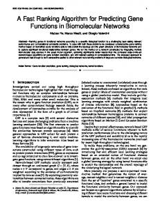
Referring back to table 2, we can also see that on mAUP and mT9P measures, the relative margin between the performance of the best ssRB and TSVM is greater on Ohsumed than on Reuters. We recall that the proportion of relevant documents per topic is sizably higher on Reuters than on Ohsumed. For example, considering mT9P scores, the difference in percentage between ssRB (for k = 1) and TSVM on the Ohsumed collection is 4% which represents 58.8% of the interval length between the worse and best mT9P performance [33.6, 40.4]. While, the difference on performance between the best ssRB (for k = 2) and TSVM on the Reuters dataset is 5.56% which represents 46.1% of the interval length [64.5, 76.5]. We further investigate the effect on the AUC measure of having less and less relevant documents in a labeled training pool where the number of irrelevant examples is kept fixed. Figure 1 illustrates this effect by showing the evolution on AUC scores of the three semi-supervised algorithms when relevant documents are gradually removed from the labeled part of the acq training set. This topic was, with earn, one of the two topics in Reuters on which ssRB did worse than the two other semi-supervised algorithms. The initial number of relevant/irrelevant documents in the labeled training set was set to respectively 9 and 81. These curves show that the decrease rate of the AUC measure of ssRB is lower than the two other semi-supervised classifiers. The loss in AUC for ssRB is less than 9% when
Reuters data set mAUP(%), r = 500 mT9P(%) 40.85 ± 0.6↓ 64.51 ± 0.4↓ 51.6 ± 0.3↓ 71.01 ± 0.2↓ ↓ 50.23 ± 0.5 70.83 ± 0.1↓ 57.32 ± 0.3 74.82 ± 0.1 59.36±0.4 76.57±0.5 57.6 ± 0.2 73.21 ± 0.3
the proportion of relevant/irrelevant documents falls from 1/9 to 1/27. This drop is about 16% for TSVM and ssLR. Figure 2, top, shows precision/recall curves on Ohsumed and Reuters collections using the same number of relevant/irrelevant documents in the respective training sets than what was used in previous experiments. In order to have an empirical upper-bound on these results we also plotted the precision/recall curves of a rankboost algorithm trained over all labeled and unlabeled examples, plus their true labels, in the different training sets. We refer to this model as RB-Fully supervised. These results confirm the previous ones as for different precision levels, the relative margin between ssRB and TSVM (or ssLR) is higher on Ohsumed than on Reuters specially for low recall rates. An explanation of these findings is that as ssRB learns a scoring function which output is supposed to rank relevant documents higher than irrelevant ones in both labeled and unlabeled training sets, its performance is less affected by fewer relevant documents.
4.3 The exponential value of labeled data We finally report on the behavior of different ranking algorithms for growing number of labeled data in the training sets. Figure 2 down, illustrates this behavior on the mAUP measures for both of datasets. The addition of new
Reuters - acq 0.94
ssRB TSVM ssLR
0.92
RB earn 85.6 ± 0.7↓ acq 81.3 ± 0.6↓ money-fx 83.8 ± 0.4↓ crude 83.4 ± 0.5↓ grain 84.5 ± 0.4↓ trade 84.9 ± 0.6↓ interest 79.9 ± 0.6↓ ship 81.2 ± 0.2↓ money-su 80.2 ± 0.3↓ sugar 78.6 ± 0.1↓
TSVM 95.9±0.1 91.6 ± 0.2 90.3 ± 0.5↓ 94.5 ± 0.4 91.1 ± 0.6↓ 91.2 ± 0.3↓ 87.6 ± 0.7↓ 85.1 ± 0.4↓ 86.2 ± 0.3↓ 86.6 ± 0.2↓
ssLR 95.4 ± 0.3 92.1±0.3 89.7 ± 0.4↓ 93.5 ± 0.4 92.4 ± 0.3↓ 90.4 ± 0.4↓ 88.3 ± 0.2↓ !84.3 ± 0.4↓ 87.3 ± 0.1↓ 85.3 ± 0.6↓
ssRB 94.8 ± 0.1 91.5 ± 0.3 92.8±0.7 95.5±0.2 93.1±0.1 92.4±0.5 90.5±0.4 89.7±0.3 91.3±0.2 90.3±0.4
0.9 0.88 0.86 AUC
Table 3: AUC measure on the 10 largest topics of the Reuters dataset for RB, TSVM, ssLR and ssRB. Semi-supervised algorithms use 90 labeled examples per topic. The remaining documents in the training set are all unlabeled.
0.84 0.82 0.8 0.78 0.76 0.74 9
8
7
6
5
4
3
# of positive examples in the labeled training set
Figure 1: AUC on Reuters category acq with respect to the number of relevant documents in the labeled training set. The number of irrelevant documents is fixed kept to 81.
Ohsumed collection 1
Reuters data set 1
RB-Fully supervised ssRB TSVM ssLR RB
0.8
RB-Fully supervised ssRB TSVM ssLR RB
0.8
Precision
0.6
Precision
0.6
0.4
0.4
0.2
0.2
0
0 0
0.2
0.4
0.6
0.8
1
0
0.2
0.4
Recall
0.6
0.8
1
Recall
(a)
(b)
0.4
0.8
0.3
0.6 mAUP
1
mAUP
0.5
0.2
0.4
0.1
0.2 ssRB TVSM ssLR RB
0 50
100
150
200
250
ssRB TVSM RB ssLR
0 300
# of labeled examples in the training set
(c)
100
150
200
250
300
# of labeled examples in the training set
(d)
Figure 2: (Top) Precision recall curves on (a) Ohsumed and (b) Reuters collections. The number of labeled examples per topic is fixed to 180 on the Ohsumed collection with a ratio of 1 relevant document for every 59 irrelevant ones, and 90 on the Reuters data set with a ratio of 1 relevant document for every 9 irrelevant ones. (Bottom) mAUP on (c) Ohsumed and (d) Reuters with respect to different labeled training size.
labeled data on each training sets respects the initial relevant/irrelevant proportion of documents on these sets. All performance curves increase monotonically with respect to the additional labeled data. The convergence rate of mAUP scores on the Reuters dataset is however faster. We expect that this is because training sets per topic on this collection contain more relevant information than Ohsumed topics.
4.4 The effect of the discount factor λ Another interesting observation here is that unlabeled examples become relatively less important as more labeled data are available. This observation is confirmed with results on figure 3 which show that for growing number of labeled training size on the Ohsumed collection, the discount factor λ for which a maximum is reached on mAUP moves away from 1. We recall that for λ = 1, unlabeled data play the same role in the training of the scoring function than labeled data.
5. CONCLUSIONS We presented a new approach to learn a boosting based, inductive ranking function in a semi-supervised setting, when both labeled and unlabeled data are available. We showed that unlabeled data do help provide a more efficient ranking function and that their effect depends on the initial labeled training size. In the most interesting case, when there are few labeled data, we empirically illustrated that unlabeled data have a large effect on the mAUP measure. We evaluated and validated our approach using two test collections. We showed through different ranking measures that the new model provides results that are superior to two semi-supervised classification algorithms on both collections. Among other things, these results confirm theoretical and empirical studies made previously in the supervised case, showing that the classification ability of classifiers is not necessarily a good indication of their ranking performance.
0.4
|Zl|=180 |Zl|=240 |Zl|=300 maxima
[8]
0.35
mAUP
[9] 0.3
[10] 0.25
[11] 0.2 0
0.2
0.4
0.6
0.8
1
λ
Figure 3: mAUP with respect to the discount factor λ for different labeled training sizes on Ohsumed. In future work, we will make the discount factor λ depend on each unlabeled example in the training set using a continuous function. The key of that study would be the choice of the function with necessary conditions allowing to take into consideration information contained on unlabeled data as best as possible. Another promising direction to explore would be the optimization of other ranking criterion than the modified AUC for learning ranking functions.
6.
ACKNOWLEDGMENTS
This work was supported in part by the IST Program of the European Community, under the PASCAL Network of Excellence, IST-2002-506778. This publication only reflects the authors’ views.
7.
[12]
[13]
[14] [15]
[16]
[17]
REFERENCES
[1] S. Agarwal. Ranking on Graph Data. In Proceedings of the 23rd International Conference on Machine Learning, pages 25-32, 2006. [2] M.-R. Amini and P. Gallinari. The Use of Unlabeled Data to Improve Supervised Learning for Text Summarization. In Proceedings of the 25th annual international ACM SIGIR, pages 105-112, 2002. [3] M.-R. Amini and P. Gallinari. Semi-Supervised Learning with Explicit Misclassification Modeling. In Proceedings of the 18th International Joint Conference on Artificial Intelligence, pages 555-560, 2003. [4] P. L. Bartlett, M. I. Jordan and Jon D. McAuliffe. Large Margin Classifiers: convex Loss, Low Noise and Convergence Rates. In Advances in Neural Information Processing Systems 16, pages 1173-1180, 2004. [5] A. Blum and T. Mitchell. Combining labeled and unlabeled data with Co-training. In Proceedings of the Workshop on Computational Learning Theory, pages 92-100, Wisconsin, USA, 1998. [6] A.P. Bradley. The use of the Area under the ROC curve in the Evaluation of Machine Learning Algorithms. Pattern Recognition, 30:1145-1159, 1997. [7] R. Caruana and A. Niculescu-Mizil. Data mining in metric space: an empirical analysis of supervised
[18]
[19] [20]
[21]
[22]
[23]
[24]
learning performance criteria. In Proceedings of the 10th ACM SIGKDD, pages 69-78, 2004. O. Chapelle, B. Sch¨ olkopf and A. Zien. Semi-Supervised Learning, MIT Press, Cambridge, MA, 2006 C. Cortes and M. Mohri. AUC optimization vs. error rate minimization. In Advances in Neural Information Processing Systems 16, pages 313-320, 2004. Y. Freund, R. Iyer, R.E. Schapire and Y. Singer. An efficient Boosting Algorithm for Combining Preferences. Journal of Machine Learning Research, 4:933-969, 2004. E. Gaussier and C. Goutte. Learning with Partially Labelled Data - with Confidence. In ICML’05 Workshop on Learning from Partially Classified Training Data (ICML’05-LPCT), pages 29-36, 2005. W. Hersh, C. Buckley, T. J. Leone and David Hickam. OHSUMED: an interactive Retrieval Evaluation and new Large Test Collection for Research. In Proceedings of the 17th annual international ACM SIGIR, pages 192-201, 1994. T. Joachims. Transductive Inference for Text Classification using Support Vector Machines. In Proceedings of 16th International Conference on Machine Learning, pages 200-209, 1999. E.L. Lehmann. Nonparametric Statistical Methods Based on Ranks. McGraw-Hill, New York, 1975. D. D. Lewis. Reuters-21578, distribution 1.0 http://www.daviddlewis.com/resources /testcollections/reuters21578/. January 1997. K. Nigam, A.K. McCallum, S. Thrun and Tom Mitchell. Text classification from labeled and unlabeled documents using EM. Machine Learning 39(2/3):127-163, 2000. S. Robertson and D.A. Hull. The TREC-9 Filtering Track Final Report. In Proceedings of the 9th Text REtrieval Conference (TREC-9). pages 25-40, 2001. I. Soboroff and S. Robertson. Building a Filtering Test Collection for TREC 2002. In Proceedings of the 26th annual international ACM SIGIR. pages 243-250, 2003. C. van Rijsbergen, Information Retrieval, Butterworths, London, 1979. J.-N. Vittaut, M.-R. Amini and P. Gallinari, Learning Classification with Both Labeled and Unlabeled Data. In Proceedings of the 13th European Conference on Machine Learning. pages 468-476, 2002. C.C. Vogt and G.W. Cottrell, Fusion Via a Linear Combination of Scores. Information Retrieval, 1(3):151-173, 1999. J. Weston, R. Kuang, C. Leslie and W.S. Noble. Protein ranking by semi-supervised network propagation. BMC Bioinformatics, special issue, 2006. D. Zhou, J. Weston, A. Gretton, O. Bousquet and B. Sch¨ olkopf. Ranking on Data Manifolds. In Advances in Neural Information Processing Systems 16, pages 169-176, 2004. D. Zhou , C.J.C. Burges and T. Tao. Transductive link spam detection. In Proceedings of the 3rd international workshop on Adversarial information retrieval on the web. pages 21-28, 2007.