Online Bayesian Multiple Kernel Bipartite Ranking
Changying Du1,2 , Changde Du3,4 , Guoping Long1 , Qing He2 , Yucheng Li1 1 Laboratory of Parallel Software and Computational Science, Institute of Software Chinese Academy of Sciences (CAS), Beijing 100190, China 2 Key Lab of Intelligent Information Processing of CAS, Institute of Computing Technology, CAS, Beijing 100190, China 3 Key Laboratory of Optical Astronomy, National Astronomical Observatories, CAS, Beijing 100012, China 4 University of Chinese Academy of Sciences, Beijing 100049, China
[email protected],
[email protected],
[email protected]
Abstract Bipartite ranking aims to maximize the area under the ROC curve (AUC) of a decision function. To tackle this problem when the data appears sequentially, existing online AUC maximization methods focus on seeking a point estimate of the decision function in a linear or predefined single kernel space, and cannot learn effective kernels automatically from the streaming data. In this paper, we first develop a Bayesian multiple kernel bipartite ranking model, which circumvents the kernel selection problem by estimating a posterior distribution over the model weights. To make our model applicable to streaming data, we then present a kernelized online Bayesian passive-aggressive learning framework by maintaining a variational approximation to the posterior based on data augmentation. Furthermore, to efficiently deal with large-scale data, we design a fixed budget strategy which can effectively control online model complexity. Extensive experimental studies confirm the superiority of our Bayesian multi-kernel approach.
1
INTRODUCTION
Aiming to learn a ranking decision function that is likely to place a positive instance before most negative ones, bipartite ranking [Agarwal and Roth, 2005; Cl´emenc¸on et al., 2008; Kotlowski et al., 2011] is especially useful for imbalanced data sets, where the area under the ROC curve (AUC) [Hanley and McNeil, 1982; Bradley, 1997; Cortes and Mohri, 2004] is a commonly used evaluation metric. Recently, several online AUC maximization algorithms with pairwise loss functions were proposed to tackle this problem when the data appears sequentially [Zhao et al., 2011a,b; Zhao and Hoi, 2012; Yang et al., 2013; Gao et al., 2013; Hu et al., 2015; Ding et al., 2015].
Furthermore, the generalization performance of online learning algorithms with pairwise loss functions have been investigated in [Wang et al., 2012; Kar et al., 2013]. Nevertheless, existing work only focus on seeking a point estimate of the decision function in a linear or predefined single kernel space, and cannot learn effective kernels automatically from the streaming data. As well known, choosing an appropriate kernel for real-world situations usually is not easy for users without enough domain knowledge. Multiple Kernel Learning (MKL) [Rakotomamonjy et al., 2008; G¨onen and Alpaydın, 2011] can circumvent such a problem by learning an optimal linear combination of a set of predefined kernels. However, conventional online MKL algorithms [Luo et al., 2010; Hoi et al., 2013; Sahoo et al., 2014] are unsuitable for a direct use since AUC is a metric represented by the sum of pairwise losses between instances from different classes. More importantly, existing online MKL methods typically maintain a point estimate of their model weights, which can be affected seriously by online outliers and usually needs a tough tuning process for their penalty parameters. Focusing on these problems, we first develop a Bayesian Bipartite Ranking model with Multiple Kernels (B2 RMK), which circumvents the kernel selection problem by estimating a posterior distribution over the model weights. Specifically, B2 RMK imposes global-local sparsity shrinkage priors on the weights of kernels and support vectors and adopts a margin-based ranking pseudo-likelihood function that mimics the pairwise hinge loss and can be expressed as a location-scale mixture of normals. Within the Bayesian formalism, the new model can automatically infer the weight penalty parameters and naturally alleviate overfitting to small training sets via model averaging over the posterior. To make our model applicable to streaming data, we then present a kernelized online Bayesian Passive-Aggressive (PA) [Crammer et al., 2006] learning framework. As far as we know, this is the first effort to perform online Bayesian learning with multiple kernels. The key of Bayesian PA
is to maintain a posterior distribution at each time step. Unfortunately, exact posterior inference of B2 RMK is intractable, so we devise an efficient data augmentation [Tanner and Wong, 1987] based variational method to approximate the posterior with mean-field assumption. Unlike most existing online MKL methods [Jin et al., 2010; Luo et al., 2010; Hoi et al., 2013], which don’t bound their model complexity and require more and more memory and computation when the data arrives sequentially, online B2 RMK only maintains two fixed-size buffers (one for positive instances, and another for negative ones) to store the learned support vectors, thus are much more efficient for large-scale data sets. When a buffer is full, we propose a principled strategy to update it, which can guarantee that the most important support vectors won’t be discarded. As in [Hu et al., 2015], smooth updating and compensation schemes are employed to further boost performance when updating the buffer. Extensive experimental studies confirm the superiority of our online Bayesian multi-kernel approach.
2
To better motivate our work, we first introduce some preliminaries, including bipartite ranking, AUC optimization and MKL. Let X = {x ∈ Rd } be the instance space, Y = {+1, −1} be the label set, and S = S+ ∪ S− be a set of training instances, where S+ and S− include N+ positive instances and N− negative instances, respectively. The goal of bipartite ranking is to learn a ranking decision function that is likely to place a positive instance before most negative ones. AUC is a commonly used evaluation metric for bipartite ranking. For a ranking decision function f : X → R, its AUC measure on S is defined as: ∑N+ ∑N− i=1
− I(f (x+ i )≤f (xj )) N+ N−
j=1
where I(π) is the indicator function that equals 1 when π is true and 0 otherwise. Since directly maximizing AUC(f ) leads to a difficult combinatorial optimization problem, in practice, the indicator function is usually replaced by its convex surrogate, e.g., pairwise hinge loss [Hu et al., 2015; Zhao et al., 2011a] and squared loss [Gao et al., 2013], which leads to minimizing the following regularized pairwise learning task [Christmann and Zhou, 2015]: ∑∑ ( ) c − ∥f ∥2H + ℓ f ; x+ i , xj 2 i=1 j=1 N+ N−
L(f ) =
f (xi ) = a⊤ ki + b
where a = [a1 , . . . , aN ]⊤ denotes the vector of weights assigned to each training instance (N = N+ + N− ); b is the bias; and ki = [K(x1 , xi ), . . . , K(xN , xi )]⊤ , where K : X × X → R is a kernel function that measures the similarities between xi and xj , j = 1, 2, . . . , N . An important problem in single kernel learning is to prespecify the kernel parameters, which is often done in an empirical way. This problem can be circumvented by using the MKL framework [Rakotomamonjy et al., 2008], which is a popular technique for learning an optimal linear combination of a set of predefined kernels. MKL algorithms basically use a weighted sum of P kernels {Km : X ×X → R}P m=1 to get the following multi-kernel ranking decision function: ( P ) P ∑ ∑ f (xi ) = a⊤ em km,i + b = em a⊤ km,i + b m=1
m=1
where km,i = [Km (x1 , xi ), . . . , Km (xN , xi )]⊤ , and em denotes the weight assigned to the m-th kernel.
PRELIMINARIES
AUC(f ) = 1 −
be written as
where ∥ · ∥H denotes the norm in Reproducing Kernel Hilbert Space (RKHS), ℓ(·) is the convex surrogate loss function and c is the regularization parameter balancing the model complexity and training errors. A kernelized ranking decision function f : X → R that is used to predict the ranking score of a test instance xi can
In the sequel, the m-th N × N kernel matrix will be denoted by Km , and the vector of ranking scores of positive instances and negative instances will be denoted by f+ and [ ⊤ ⊤ ]⊤ f− , respectively, and f = f+ f− .
3 BAYESIAN MULTIPLE KERNEL BIPARTITE RANKING In this section, we formulate a probabilistic model for multi-kernel bipartite ranking. We impose a fairly general global-local shrinkage prior on the sample weights and kernel combination weights to keep the sparsity of them. Since pairwise hinge loss makes traditional Bayesian analysis hard, we then define a margin-based ranking pseudolikelihood function to overcome this situation. After introducing a set of augmented variables and making the meanfield assumption, the intractable inference problem of our model can be transformed into a tractable one. 3.1
BAYESIAN SPARSITY SHRINKAGE PRIOR
Similar as in kernelized SVM, the sample weights a is often expected to be sparse for selecting support vectors actually needed in decision function. From the Bayesian perspective, a fairly general global-local shrinkage prior is the Three Parameter Beta Normal (T PBN ) [Armagan et al., 2011], which favors strong shrinkage of small signals while having heavy tails to avoid over-shrinkage of the larger signals. Thus, concentrated at zero, T PBN can yield sparse model representations by suppressing unnecessary support vectors. In this paper, we select T PBN as the sparsity shrinkage prior due to its better mixing properties than
priors such as spike-slab and Laplace. Besides, T PBN works well for high-dimensional settings since it can specify global ∏N and local properties independently. Assuming a ∼ i=1 T PBN (ai |αa , βa , ϕ), we have the following hierarchical prior: ∼
N (ai |0, λi ),
λi |ξi
∼
Γ(λi |αa , ξi ),
ξi |ϕ ∼ Γ(ξi |βa , ϕ),
ϕ|η
∼
Γ(ϕ|1/2, η),
η ∼ Γ(η|1/2, 1),
where Γ(·) is the Gamma distribution (with shape-rate parameterization). Note that sample-level sparsity can be tuned by assigning suitable values to the hyper-parameters (αa , βa ). Setting αa = βa = 0.5, a special case of T PBN corresponds to the horseshoe prior. Similarly, sparsity on kernel combination weights e = [e1 , . . . , eP ]⊤ is also desirable for better interpretability. ∏P So, we assume e ∼ m=1 T PBN (em |αe , βe , ρ), involving latent variables ωm , φm and τ . Kernel-level sparsity can also be tuned by changing (αe , βe ). With the above priors on model weights, we assume the ranking scores of our B2 RMK model have the following distributions, P ∏ N ∏
( ) N gmi |a⊤ km,i , υ −1 ,
m=1 i=1
f+ |e, G, b, c ∼
N+ ∏
L(y|f ) =
∏
f− |e, G, b, c ∼
( ) N fi |e⊤ g·i + b, c−1 , ( ) N fj |e⊤ g·j + b, c−1 ,
j=1
( ) where υ ∼ Γ (υ|αυ , βυ ), b|γ ∼ N b|0, γ −1 , γ ∼ Γ (γ|αγ , βγ ), c ∼ Γ (c|αc , βc ). The intermediate variables gmi (m = 1, . . . , P, i = 1, . . . , N ) are introduced to make the inference procedures efficient. The P × N matrix of intermediate variables is denoted by G, and the m-th row and i-th column of G by gm· and g·i , respectively. In the sequel, all hyper-parameters will be denoted by Υ = {αa , βa , αe , βe , αυ , βυ , αγ , βγ , αc , βc }, while the priors by Ψ = {λ, ξ, ϕ, η, ω, φ, ρ, τ, υ, γ, c} and the remaining variables by Ω = {a, b, e, G, f+ , f− }. 3.2
MARGIN-BASED RANKING LIKELIHOOD
Several loss functions are available for bipartite ranking. Among them, pairwise hinge loss is the tightest convex upper bound on the rank loss, which is beneficial for better performance and faster convergence. Specifically, the pairwise hinge loss on data set S can be written as ℓ(f ; S) =
N+ N− ∑ ∑ i=1 j=1
exp (−2max(0, 1 − fi + fj )) ,
where y is the label vector and has been divided out. With T PBN priors and the above margin-based ranking pseudo-likelihood, we can get the following pseudo posterior distribution using Bayes’ rule p(Ψ, Ω|y) = L(y|f )p(Ω|Ψ)p(Ψ)/p(y|Υ), where p(y|Υ) is the normalization constant. Note that it is hard to compute p(Ψ, Ω|y) analytically due to the max function in L(y|f ). Fortunately, we can re-express L(y|f ) as the product of N+ · N− location-scale mixtures of normals (see Supplement Section A) based on data augmentation idea [Tanner and Wong, 1987] ( ) 2 N+ N− ∫ ∞ exp (θij +1−fi +fj ) ∏ ∏ −2θij √ L(y|f ) = dθij , (1) 2πθij i=1 j=1 0 where θij is the augmented variable. In the following, the matrix of augmented variables will be denoted by θ, and the i-th row and j-th column of θ by θi· and θ·j , respectively. (1) indicates that the posterior distribution p(Ψ, Ω|y) can be expressed as the marginal of a higher-dimensional distribution that includes the augmented variables. Therefore, the augmented posterior distribution has the form
i=1 N−
N+ N− ∏ ∏ i=1 j=1
ai |λi
G|a, {Km }P m=1 , υ ∼
which does not lend itself to a convenient description of a likelihood function. To overcome this situation, we propose to define a margin-based ranking pseudo-likelihood
( ) − max 0, 1 − f (x+ i ) + f (xj ) ,
p(Ψ, Ω, θ|y) =
L(y, θ|f )p(Ω|Ψ)p(Ψ) , p(y|Υ)
(2)
where the unnormalized joint distribution of y and θ conditioned on f is ( ) N+ N− ∏ ∏ 1 (θij + 1 − fi + fj )2 √ L(y, θ|f ) = exp . −2θij 2πθij i=1 j=1 3.3
VARIATIONAL APPROXIMATE INFERENCE
Directly solving for the augmented posterior is intractable due to the normalization constant p(y|Υ), thus we appeal to the mean-field variational approximate Bayesian inference method, which is generally much more efficient than the Markov Chain Monte Calo (MCMC) based sampling methods. Specifically, we assume there are a family of factorable and free-form variational distributions q(Ψ, Ω, θ) = q(λ)q(ξ)q(ϕ)q(η)q(ω)q(φ)q(ρ)q(τ )q(υ) ·q(γ)q(c)q(a)q(b, e)q(G)q(f+ )q(f− )q(θ), and the objective is to get the optimal one which minimizes the Kullback-Leibler (KL) divergence between the approximating distribution and the target posterior, i.e., min q(Ψ,Ω,θ)∈P
KL (q(Ψ, Ω, θ)∥p(Ψ, Ω, θ|y)) ,
where P is the space of probability distributions. To this end, we first initialize the moments of all factor distributions of q(Ψ, Ω, θ) appropriately and then iteratively optimize each of the factors in turn using the current estimates for all of the other factors. It can be shown that when keeping all other factors fixed the optimal distribution q ∗ (a) satisfies ∗
q (a) ∝
exp{E−a [log p(Ψ, Ω, θ, {Km }P m=1 , y)]},
p(Ψ, Ω, θ, {Km }P m=1 , y) = L(y, θ|f )p(f |e, G, b, c)p(G|a, {Km }P m=1 , υ) ·p(a|λ)p(e|ω)p(b|γ)p(λ|ξ)p(ξ|ϕ)p(ϕ|η)p(η) ·p(ω|φ)p(φ|ρ)p(ρ|τ )p(τ )p(υ)p(γ)p(c). Expanding the right side of (3) and ignoring the terms unrelated to a, we can further get1 q ∗ (a) ∝ exp{E−a [log p(G|a, {Km }P m=1 , υ) + log p(a|λ)]} ( ( ) ) ∑P ⊤ = N Σa ⟨υ⟩ Km ⟨gm· ⟩ , Σa , m=1
)−1 ( ∑ P −1 + ⟨Λ ⟩ and Λ−1 where Σa = ⟨υ⟩ m=1 Km K⊤ m λ λ = diag(λ)−1 . Similarly, we can also get ( ) [ ]⊤ q ∗ (b, e) = N Σ(b,e) ⟨c⟩ 1, ⟨G⟩⊤ ⟨f ⟩, Σ(b,e) , N ∏
( ( )−1 ) N µg·i , ⟨c⟩⟨ee⊤ ⟩ + ⟨υ⟩I ,
i=1 N− (∑ )−1 ) q (f+ ) = N µf+ , ⟨Λ−1 , θ·j ⟩ + ⟨c⟩I ∗
(
j=1
(
N+ (∑ )−1 ) q ∗ (f− ) = N µf− , ⟨Λ−1 ⟩ + ⟨c⟩I , θi· i=1
q ∗ (θ) =
∏∏ N+ N−
GIG
i=1 j=1
where Σ(b,e) =
[ ⟨c⟩N + ⟨γ⟩, ⟨c⟩⟨G⟩1,
(1 2
4 ONLINE B2 RMK LEARNING
(3)
where E−a denotes the expectation with respect to p(Ψ, Ω, θ) over all variables except for a, and p(Ψ, Ω, θ, {Km }P m=1 , y) is the joint distribution of data and all variables, which has the following form
q ∗ (G) =
Note that, θ −1 is the element-wise inversion of θ, and G+ (G− ) denotes the part of G corresponding to positive (negative) instances. The detailed derivations of the above equations together with the equations for all other variables can be found in the Supplement Section B.
) , 1, ⟨(1 − fi + fj )2 ⟩ ,
]−1 ⟨c⟩1⊤ ⟨G⊤ ⟩ , ⟨c⟩⟨GG⊤ ⟩ + ⟨Λ−1 ω ⟩
µg·i = Σg·i (⟨c⟩ (⟨fi ⟩⟨e⟩ − ⟨be⟩) + ⟨υ⟩K⊤ i ⟨a⟩), µf+ = Σf+ (N− 1+⟨θ −1 ⟩ (⟨f− ⟩ + 1)+⟨c⟩(⟨G⊤ + ⟩⟨e⟩+⟨b⟩1)),
The above batch B2 RMK model still suffers from efficiency problems, e.g., huge memory consumption in dealing with large data sets and time-consuming re-training when the data appears sequentially. Online Passive-Aggressive (PA) [Crammer et al., 2006] learning is a principled way to solve such problems. However, it is less explored under the Bayesian framework. Here, we present a fixed budget strategy to conduct online multiple kernel PA learning in Bayesian manner. Our method can be seen as an extension of the linear framework in [Shi and Zhu, 2014], which studied online max-margin topic models. In the online setting, what we truly care about is how to update the current model, on the arrival of a new data. So, assume we already have an existing B2 RMK model at the t-th trial. In the updating of the kernel-based ranking decision function, the main problem is to compute the Gram matrix of pairwise kernel evaluations between the historical instances and new arriving instance, and we have to store all the received historical instances, making it impractical for large-scale online learning tasks. We address this challenge by maintaining only a small number of received historical instances. Specifically, we define two buffers Bt+ and Bt− of size |Bt+ | and |Bt− |, for storing the learned important positive and negative support vectors at the t-th trial, respectively. These support vectors in Bt+ and Bt− are essential for constructing the ranking decision function at the (t+1)-th trial, thus are expected to keep track of the global information of the decision boundary. To this end, existing online MKL methods [Luo et al., 2010; Hoi et al., 2013] typically assume an infinite buffer. However, their naive treatment of storing all received historical instances, requires more and more memory and computation when the data arrives sequentially. On the contrary, we control the computational complexity of our Online B2 RMK (OB2 RMK) model by fixing the buffer size to an appropriate value, assuming that the performance of OB2 RMK increases gradually with the increase of the buffer and it will be saturated when the buffer is large enough. As will be seen in the experimental section, such assumptions are well validated. Overall, the proposed OB2 RMK consists of two key modules, i.e., buffer update and model update.
µf− = Σf− (⟨θ −1 ⟩⊤ (⟨f+ ⟩ − 1)−N+ 1+⟨c⟩(⟨G⊤ − ⟩⟨e⟩+⟨b⟩1)).
4.1
1 Here ⟨·⟩ means the expectation operator, e.g., ⟨υ⟩ means the expectation of υ over its current optimal variational distribution.
How to maintain the buffers with the most informative support vectors to get better generalization performance is a
UPDATE BUFFER
key challenge. Traditionally, First-In-First-Out (FIFO) and Reservoir Sampling (RS) are two typical stream oblivious policies to update the buffers and have demonstrated their effectiveness in online linear AUC maximization [Zhao et al., 2011a]. However, FIFO and RS will cast off the important support vectors, thus will degrade the performance of the online learning algorithms. Compared with linear algorithms, this adverse impact will be more intense in the kernel-based algorithms which work with the Gram matrix of pairwise kernel evaluations [Yang et al., 2013; Hu et al., 2015]. In the following, we will propose a novel strategy to update the buffers for OB2 RMK, aiming to preserve the most important support vectors. For the incoming new instance (x⋆ , y⋆ ), instead of counting its pairwise losses with all support vectors in the opposite buffer which is easily affected by outliers, we only count the pairwise losses with its k-nearest opposite support vectors Xk . This allows us to utilize the local information around x⋆ and improve the robustness of the ranking decision function [Hu et al., 2015]. When the buffers Bt+ and Bt− are not full, the incoming new instance will be put into one of the buffers directly, thus the pairwise hinge loss at the (t+1)-th trial is ℓ(f ; x⋆ , Xk ) = ∑ ( ) kj=1 max 0, 1 − f (x⋆ ) + f (x− j ) , y⋆ = 1, ∑k max (0, 1 − f (x+ ) + f (x )) , y = −1. ⋆ ⋆ i i=1 When either buffer is full, one of the instances in this buffer should be discarded, to accommodate the incoming new instance. Recall that the T PBN prior concentrates at zero, thus a positive (negative) support vector xi is likely to have a positive (negative) weight ai to attain a discriminative decision function. Supposing Bt+ (Bt− ) is full, we first search for a support vector xr which has the smallest (largest) weight in the buffer. Instead of discarding xr directly, we put xr and x⋆ together to count the pairwise losses between them and Xk . This compensation scheme guarantees the useful information of xr can be fully utilized before it is discarded. Hence, the pairwise hinge loss at the (t+1)-th trial is ℓ(f ; x⋆ , xr , Xk ) = ∑k − j=1 {max(0, 1 − f (x⋆ ) + f (xj )) + max(0, 1 − f (xr ) + f (x− j ))}, y⋆ = 1, ∑ k + i=1 {max(0, 1 − f (xi ) ++ f (x⋆ )) + max(0, 1 − f (xi ) + f (xr ))}, y⋆ = −1. Concisely, the pairwise hinge loss at the (t+1)-th trial can be uniformly written as ˜
ℓ(f ; x⋆ , Bt ) =
˜
N+ N− ∑ ∑ i=1 j=1
(
max 0, 1 −
f (x+ i )
+
f (x− j )
)
,
˜+ and N ˜− are the number where Bt = Bt+ ∪ Bt− , and N of positive and negative instances, respectively, in counting the pairwise hinge loss at the (t+1)-th trial. For example, ˜+ = 1, N ˜− = k when y⋆ = 1 and Bt+ was not we have N ˜+ = 2, N ˜− = k when y⋆ = 1 full (i.e., without xr ), and N + and Bt was full (i.e., with xr ). 4.2
UPDATE MODEL
In online B2 RMK, the model parameters a, b and e should vary with t, to update the ranking decision function. Note that the dimensionality of a will increase until the buffers are full, whereas b and e are always fixed-size. 4.2.1
Priors
Let pt (at , b, e) denote the posterior distribution of (a, b, e) at the t-th trial, which will become a prior distribution at the (t+1)-th trial. Assuming a⋆ is the corresponding weight of x⋆ at the (t+1)-th trial. After imposing a T PBN prior on a⋆ , i.e., a⋆ |αa⋆ , βa⋆ , ϕ⋆ ∼ T PBN (a⋆ |αa⋆ , βa⋆ , ϕ⋆ ), we have the hierarchical priors: a⋆ |λ⋆ ∼ N (a⋆ |0, λ⋆ ), λ⋆ |ξ⋆ ∼ Γ(λ⋆ |αa⋆ , ξ⋆ ), ξ⋆ |ϕ⋆ ∼ Γ(ξ⋆ |βa⋆ , ϕ⋆ ), ϕ⋆ |η⋆ ∼ Γ(ϕ⋆ |1/2, η⋆ ) and η⋆ ∼ Γ(η⋆ |1/2, 1). The prior distributions of G, f+ , f− , υ and c are omitted here as they are similar as in B2 RMK. Now let ˜ = {αa , βa }, Ψ ˜ = {λ⋆ , ξ⋆ , ϕ⋆ , η⋆ } and Ω ˜ = Υ ⋆ ⋆ {f+ , f− , G, υ, c} for notational simplicity. 4.2.2
Posterior Updating
˜ and Ω ˜ actually are random variables, we Since a, b, e, Ψ have to average the loss ℓ(f ; x⋆ , Bt ) over their joint distribution. Let Ep(a,b,e,Ψ, ˜ Ω) ˜ denote the expectation over ˜ Ω), ˜ then we define the following expected p(a, b, e, Ψ, pairwise hinge loss at the (t+1)-th trial: ˜ Ω)) ˜ = R(p(a, b, e, Ψ, ˜ ˜ N − ∑+ N ∑ Ep(a,b,e,Ψ, ˜ Ω) ˜ [max (0, 1 − fi + fj )]. i=1 j=1
Note that, expected pairwise hinge loss is an upper bound of the pairwise hinge loss of the expected bipartite ranking model by Jensen’s inequality, and is more convenient for our inference as shown below. Now we can infer the new posterior distribution pt+1 (a, b, e) on the arrival of the new data (x⋆ , y⋆ ) by solving the following optimization problem: min p(a,b,e)∈P
KL (p(a, b, e)∥pt (at , b, e)p(a⋆ )) ˜ Ω)), ˜ +2C · R(p(a, b, e, Ψ,
(4)
where C is a positive regularization parameter, the constant ˜ Ω)) ˜ is the ex2 is just for convenience, and R(p(a, b, e, Ψ, pected pairwise hinge loss at the (t+1)-th trial. Intuitively,
we find a posterior distribution pt+1 (a, b, e) in the feasible zone that is not only close to pt (at , b, e)p(a⋆ ), but also [ ]⊤ has small loss at the new trial. Note that a = a⊤ t a⋆ at the (t+1)-th trial, but if Bt+ (Bt− ) is already full and y⋆ = 1 (y⋆ = −1), the weight vector at has been truncated one dimension before the optimization (4) to accommodate a⋆ , which corresponds to an updating of the buffer. Directly optimizing (4) with R is difficult and inefficient. Here we regard Lt+1 (y|a, b, e) = ˜+ N ˜− { } N ∏ ∏ exp −2C · Ep(Ψ, ˜ Ω) ˜ [max(0, 1 − fi + fj )] , i=1 j=1
as the unnormalized pseudo-likelihood of label vector y, then (4) can be rewritten as min p(a,b,e)∈P
KL (p(a, b, e)∥pt (at , b, e)p(a⋆ )) −Ep(a,b,e) [log(Lt+1 (y|a, b, e))].
It is straightforward to verify that the solution of this information theoretical optimization problem is p(a, b, e) =
pt (at , b, e)p(a⋆ )Lt+1 (y|a, b, e) , ˜ p(y|Υ)
˜ is the normalization constant, and the poswhere p(y|Υ) terior at the t-th trail pt (at , b, e) becomes a prior. Since it ˜ Ω) ˜ is hard to compute the expectation with respect to p(Ψ, in Lt+1 (y|a, b, e), we can regard the posterior distribution p(a, b, e) as the marginal of a higher-dimensional distribu˜ and Ω. ˜ Note that Ψ ˜ and Ω ˜ tion that includes variables Ψ will play only an auxiliary role in the inference procedure. ˜ Therefore, the higher-dimensional distribution of a, b, e, Ψ ˜ and Ω at the (t+1)-th trial satisfies the following form: ˜ ˜ ˜ Ω) ˜ = pt (at , b, e)p(a⋆ )p(Ψ, Ω)Lt+1 (y|f ) , pt+1 (a, b, e, Ψ, ˜ p(y|Υ) ˜
Lt+1 (y|f ) =
˜
N+ N− ∏ ∏
exp (−2C · max(0, 1 − fi + fj )) ,
i=1 j=1
which is intractable to compute analytically due to the max function in it. Similar as in B2 RMK, where data augmentation presents an elegant way to deal with the challenging posterior inference problem, we transform Lt+1 (y|f ) into ˜+ · N ˜− location-scale mixtures of normals: the product of N ) ( (θij +C(1−fi +fj ))2 ˜+ N ˜− ∫ N ∞ exp ∏ ∏ −2θij √ Lt+1 (y|f ) = dθij . 2πθij i=1 j=1 0 Now Lt+1 (y|f ) can also be seen as the marginal of the higher-dimensional distribution
Lt+1 (y, θ|f ) =
˜+ N ˜− N exp ∏ ∏
(
i=1 j=1
(θij +C(1−fi +fj ))2 −2θij
√ 2πθij
) ,
and the complete posterior distribution at the (t+1)-th trial can be expressed as ˜ Ω, ˜ θ) = pt+1 (a, b, e, Ψ, ˜ Ω)L ˜ t+1 (y, θ|f ) pt (at , b, e)p(a⋆ )p(Ψ, . ˜ p(y|Υ) 4.2.3
Approximate Inference
We then make the variational approximate inference for ˜ Ω, ˜ θ). Specifically, assume there are a fampt+1 (a, b, e, Ψ, ily of factorable and free-form variational distributions ˜ Ω, ˜ θ) = qt+1 (a, b, e, Ψ, qt+1 (a)qt+1 (b, e)qt+1 (λ⋆ )qt+1 (ξ⋆ )qt+1 (ϕ⋆ )qt+1 (η⋆ ) ·qt+1 (υ)qt+1 (c)qt+1 (G)qt+1 (f+ )qt+1 (f− )qt+1 (θ), and the goal is to get the optimal one which minimizes ˜ Ω, ˜ θ)∥pt+1 (a, b, e, Ψ, ˜ Ω, ˜ θ)) between KL(qt+1 (a, b, e, Ψ, the approximating distribution and the target posterior. Following similar derivations as in B2 RMK model, we can infer the optimal distributions for all involved variables at the (t+1)-th trial, and the detailed descriptions are shown in Supplement Section C.
5 CONVERGENCE, COMPLEXITY AND PREDICTION In both B2 RMK and OB2 RMK, the inference mechanism sequentially updates the approximate posterior distributions of the model parameters and the augmented parameters until convergence, which is guaranteed because the KL divergence is convex with respect to each of the factors. Rather than addressing the high-dimensionality problem directly, our kernel-based approach always transforms the original data into kernel matrices whose sizes only depend on the number of instances. Meanwhile, our online algorithm can naturally overcome the memory consumption challenge posed by large training sets. For B2 RMK, the computational complexity for transforming original data into kernel matrices {Km }P m=1 is O(N 2 P d), where d is the dimensionality of the original ∑P data. Note that m=1 Km K⊤ m should be cached before starting inference to reduce the computation. The computational complexity for each iteration of the variational inference on training data is O(N 3 + P 3 ), where the matrix inversions for computing the covariances Σa and Σb,e consume O(N 3 ) and O(P 3 ) computation, respectively. Note that we can explore the symmetric positive semi-definite property to accelerate these matrix inversions.
For OB2 RMK, the computational complexity for the construction of P kernel matrices {Km }P m=1 at the t-th tri˜ P d), where |Bt | = |Bt+ | + |Bt− | and al is O(|Bt |N ˜ = N ˜+ + N ˜− . The computational complexity for N each iteration of the variational inference during training is O(|Bt |3 + P 3 ), which indicates that the computational complexity of OB2 RMK will be limited by the buffer size |Bt | when P is given. After obtaining the approximate posterior distributions q ∗ (a) and q ∗ (b, e), the ranking score for a new instance xnew can be calculated by: (∑ ) P fnew = ⟨a⟩⊤ m=1 ⟨em ⟩km,new + ⟨b⟩.
Table 1: Details of the data sets used in our experiments. Datasets #instances sonar 208 glass 214 heart 270 bupaliver 345 ionosphere 351
Datasets #instances svmguide2 391 diabetes 768 fourclass 862 german 1000 splice 1000
Datasets #instances svmguide3 1243 segment 2310 satimage 4435 spambase 4601 usps 9298
EXPERIMENTS
• Three batch learning algorithms, including SVMperf for ordinal regression (SVM-OR) [Joachims, 2006], a bipartite ranking model with univariate logistic loss (Uni-Log) [Kotlowski et al., 2011] and least square SVM (LS-SVM); • Several state-of-the-art online AUC maximization algorithms, including one-pass AUC optimization (OPAUC) [Gao et al., 2013], kernelized online imbalanced learning (KOIL) algorithm with fixed budgets [Hu et al., 2015] and a bounded kernel-based online learning algorithm (Projectron++) [Orabona et al., 2009]; • A latest online multiple kernel classification (OMKC) algorithm with infinite buffer size, which doesn’t bound its model complexity, thus requires more and more computational resources when the data arrives sequentially [Hoi et al., 2013]. 6.1
EXPERIMENTAL TESTBED AND SETUP
We conduct experiments on a variety of data sets obtained from the UCI and the LIBSVM websites, as summarized in Table 1. To be consistent with previous studies [Gao et al., 2013; Hu et al., 2015], the features have been scaled to [−1, 1] for all data sets, and multi-class data sets have been transformed into class-imbalanced binary ones. On each data set, we conduct four independent trials of 5-fold cross validation for all the algorithms, where four folds of the data are used for training while the rest for test in each trial. The averaged AUC value over these 20 runs is reported. For kernelized methods, we predefine a pool of 18 kernel functions on all features, including Gaussian kernels with 13 different widths {2−6 , 2−5 , . . . , 26 } and polynomial kernels
6.2
PERFORMANCE EVALUATION
6.2.1
Batch Learning
Though we mainly focus on online learning, we also briefly compare the proposed B2 RMK with three batch methods. We force sparsity at both sample-level and kernel-level by imposing sparsity-inducing priors (T PBN ) on the sample weights and kernel weights, respectively. Specifically, the hyper-parameters of the proposed B2 RMK are set to (αa , βa ) = (αe , βe ) = (0.5, 0.5), (αυ , βυ ) = (αc , βc ) = (10+2 , 10−2 ) and (αγ , βγ ) = (10−2 , 10−2 ) for all data sets, while 5-fold cross validation is conducted on training sets to choose a better regularization parameter from 2[−10:10] for other methods. The averaged AUC values of these batch algorithms are listed in Table 2, which show that B2 RMK performs significantly better than the competitors on 3 out of 5 data sets. Figure 1 illustrates the kernel weights and sample weights obtained by B2 RMK on ‘fourclass’ data set, which show that our model can effectively identify the key kernels and support vectors that are actually needed. Table 2: Average AUC of batch learning methods. Methods
diabetes
fourclass
german
splice
usps
SVM-OR Uni-Log LS-SVM B2 RMK
.832±.032 .833±.032 .832±.033 .832±.028
.831±.031 .829±.031 .831±.031 1.000±.000
.793±.035 .799±.034 .799±.034 .795±.027
.924±.009 .921±.011 .925±.009 .936±.012
.963±.005 .964±.004 .963±.005 .999±.001
200
500
0.4
1.5
0.35 1 0.3
Sample weights
In this section, we present extensive experimental results on real data sets to demonstrate the effectiveness of the proposed B2 RMK and OB2 RMK with fixed budgets. Specifically, we compare them with the following algorithms:
Kernel weights
6
with 5 different degrees {1, 2, . . . , 5}. Following [G¨onen, 2012], all kernel matrices are normalized to have unit diagonal entries, i.e., spherical normalization, which can be done online. Note that our Bayesian multi-kernel approach infers model parameters automatically via posterior inference rather than time-consuming grid search. Though we still have to specify the hyper-parameters, they are fixed for all 15 data sets without re-adjustment on each data set.
0.25 0.2 0.15
0.5
0
-0.5
0.1 -1 0.05 -1.5
0 2
4
6
8
10
Index of kernel
(a)
12
14
16
18
0
100
300
400
600
Index of training instances
(b)
Figure 1: (a) Kernel weights and (b) sample weights obtained by B2 RMK on ‘fourclass’ data set.
For KOIL updated by RS++ or FIFO++, we set the learning rate η = 0.01 and select the penalty parameter C from 2[−10:10] as suggested in their paper. For OPAUC, we select the learning rate parameter η and the regularization parameter λ from 2[−12:10] and 2[−10:2] , respectively. For Projectron++, we select the parameter of projection difference η from 2[−10:10] . For OMKC, we adopt the deterministic updating and combination strategy, and the discount weight parameter β and smoothing parameter δ are fixed to 0.8 and 0.01, respectively. For OB2 RMK, we initially conduct B2 RMK on the half fold of training data to get the posterior distribution p(a, b, e). Then the hyper-parameters of OB2 RMK are set to (αa⋆ , βa⋆ ) = (αυ , βυ ) = (αc , βc ) = (1, 1). The parameter k is fixed to 3, and the regularization parameter C is chosen from {0.1, 1, 3}. Furthermore, to provide KOIL and Projectron++ with multiple kernel information, we also run them with an unweighted combination of all the kernels as well as the best kernel among the pool of kernels. The symbols u and ∗ marked on the upper right corner are used for denoting them, respectively. All buffer sizes for KOIL and OB2 RMK are set to 100.
6.3
The default values of parameter C, the buffer size and the number of iterations for each online updating are 1, 100 and 30 respectively. When we study one of them through varying its values, the other two are fixed to their default values. First, from Figure 2 we observe that the performance of OB2 RMK increases gradually with the increase of the buffer size and it is saturated when the size is relatively large, which is consistent with the observations in [Zhao et al., 2011a; Hu et al., 2015]. Then, we can conclude from Figure 3 (a) that the regularization parameter C should not be too large, whereas there is a relatively broad range between [10−3 , 1] where OB2 RMK achieves good results. Finally, Figure 3 (b) shows that OB2 RMK converges rapidly, and typically stable results can be attained within 30 iterations. 1
1
0.95
0.95
0.9
0.9
0.85
0.85
0.8 0.75 0.7
0.8 0.75 0.7
0.65
0.65
0.6 0.55
0.6
bupaliver ionosphere svmguide2
0.5 0.45
3
40
70 100 The buffer size
130
german splice segment
0.55 0.5
160
3
(a) Small data sets
50
100
200 300 The buffer size
400
500
(b) Large data sets
Figure 2: Average AUC of OB2 RMK vs. buffer size. 1
1
0.95
0.95
0.9
0.9
0.85 0.85
0.8
Average AUC
Table 3 summarizes the average AUC values of the compared online algorithms. We also list the performance of the proposed batch B2 RMK in the last column for reference. Several observations can be drawn as follows. First, by comparing the proposed OB2 RMK algorithm against the other online algorithms, we can find that the OB2 RMK performs considerably better on most data sets. In particular, the AUC values of OB2 RMK significantly surpass the baseline algorithms on some data sets. For example, on ‘bupaliver’, the AUC values for the baseline algorithms are lower than 71%, while OB2 RMK is able to achieve 75.8%. Secondly, online multiple kernel learning algorithms show better AUC performance than the single kernel and linear online learning algorithms on most data sets. This demonstrates the power of multiple kernel learning methods in classifying real-world data sets. Thirdly, OPAUC achieves fairly comparable or even better results than kernel-based algorithms on the data sets of ‘svmguide2’ and ‘german’. We attribute this to the fact that a linear algorithm is enough to achieve good performance on some data sets, while the kernel-based algorithms may be easily affected by outliers. Finally, by examining the proposed OB2 RMK algorithm against the online multiple kernel learning algorithm OMKC(D,D) with infinite buffers, we can find that the
SENSITIVITY ANALYSIS
Average AUC
In real world online learning problems, there is usually very few training data at the beginning, and it is required to maintain a dynamic model with the sequentially arriving data. Since revisiting historical data is expensive for online algorithms, we cannot do cross validation on the entire training set. As such, we assume a half of one fold in the training data is available in a batch manner, and all algorithms tune their parameters on them.
OB2 RMK algorithm tends to outperform the OMKC(D,D) algorithm on most data sets. This encouraging result shows that the OB2 RMK algorithm with fixed buffer size is able to maintain an accurate sketch of historical training examples by exploring the compensation scheme.
0.8
0.75
Average AUC
Online Learning
Average AUC
6.2.2
0.7 0.65 0.6
0.75 0.7 0.65
svmguide3 ionosphere glass svmguide2 bupaliver
0.55 0.5 0.45 0.4 10^−3
10^−2
diabetes ionosphere glass svmguide2 bupaliver
0.6 0.55 0.5
10^−1
1 C
10^1
10^2
1
10^3
(a)
2
3
5 10 20 Number of iterations
30
40
50
(b) 2
Figure 3: Average AUC of OB RMK when different (a) parameter C and (b) number of iterations are used.
7 RELATED WORK Online pairwise learning has gained increasing attention recently. In [Zhao et al., 2011a], a buffer sampling based linear Online AUC maximization (OAM) model was proposed. In [Hu et al., 2015], the Kernelized Online Imbal-
Table 3: Average AUC values (mean±std) on a variety of data sets. •/◦ indicates that OB2 RMK is significantly better/worse than the corresponding method (pairwise t-tests at 95% significance level). Datasets
OB2 RMK
∗ u ∗ u KOILu Projectron++∗ RS++ KOILRS++ KOILFIFO++ KOILFIFO++ OMKC(D,D) Projectron++
sonar
.915±.044
.865±.050• .847±.051•
.865±.050•
.850±.049•
.916±.036
.713±.082•
.825±.071•
.813±.082• .942±.034◦
glass
.896±.035
.842±.050• .784±.053•
.839±.052•
.785±.054•
.856±.071•
.582±.098•
.763±.066•
.822±.059• .898±.034
heart
.895±.050
.893±.057
.894±.057
.895±.056
.854±.075•
.773±.056•
.806±.055•
.893±.051
bupaliver
.758±.058
.703±.056• .689±.062•
.707±.054•
.690±.059•
.654±.074•
.511±.020•
.587±.053•
.685±.068• .755±.061
.895±.056
OPAUC
B2 RMK
.905±.053◦
ionosphere
.982±.012
.982±.012
.971±.015•
.982±.012
.974±.018•
.969±.021•
.850±.041•
.898±.040•
.826±.075• .980±.012
svmguide2
.943±.040
.939±.033
.924±.032•
.942±.032
.919±.038•
.921±.043•
.790±.065•
.836±.040•
.922±.035• .942±.035
diabetes
.824±.028
.808±.039• .789±.045•
.817±.036•
.798±.038•
.789±.022•
.574±.047•
.681±.041•
.742±.067• .832±.028◦
fourclass
1.000±.000 .987±.039• .999±.001
.987±.039•
.999±.001
.999±.001
.815±.045•
.998±.002•
.830±.021• 1.000±.000
german
.768±.029
.760±.039• .724±.046•
.761±.042•
.733±.041•
.723±.042•
.544±.030•
.625±.031•
.749±.043• .795±.027◦
splice
.894±.019
.886±.021• .869±.018•
.887±.019•
.872±.024•
.906±.022◦
.701±.030•
.797±.024•
.865±.020• .936±.012◦
svmguide3
.732±.023
.686±.039• .620±.052•
.685±.051•
.625±.045•
.725±.034•
.503±.005•
.626±.031•
.715±.042• .807±.026◦
segment
.984±.005
.975±.006• .959±.011•
.975±.006•
.957±.009•
.970±.006•
.789±.036•
.962±.010•
.895±.016• .998±.001◦
satimage
.978±.006
.958±.006• .973±.007•
.956±.008•
.973±.007•
.974±.003
.903±.016•
.937±.006•
.848±.028• .991±.002◦
spambase
.944±.010
.938±.016• .922±.017•
.938±.009•
.927±.015•
.958±.007◦
.866±.021•
.893±.019•
.941±.009
usps
.990±.003
.985±.004• .988±.004
.984±.005•
.988±.003
.986±.002
.867±.030•
.976±.003•
.957±.003• .999±.001◦
12/3/0
12/3/0
9/4/2
15/0/0
15/0/0
win/tie/loss
12/3/0
12/3/0
anced Learning (KOIL) algorithm extended OAM to the nonlinear case with a predefined single kernel. Both of them provided regret bound based on pairwise hinge loss. [Ding et al., 2015] extended OAM with adaptive gradient method which can exploit the knowledge of historical gradients. Besides, [Gao et al., 2013] proposed a linear one-pass AUC optimization model which scans through the training data only once owing to the use of squared loss. A more recent squared loss based algorithm, named OPERA, was proposed in [Ying and Zhou, 2015], where a non-strongly convex objective was formulated in an unconstrained reproducing kernel Hilbert space. All the aforementioned methods seek point estimates of the decision function in a linear or single kernel space. On the other hand, recent years witnessed the efforts on online extensions of multiple kernel learning due to its efficiency constrictions. Luo et al. [Luo et al., 2010] first introduced an Online Multiclass Multi-kernel (OM2) classification algorithm with hinge loss. In [Hoi et al., 2013], Hoi et al. proposed several Online Multiple Kernel Classification (OMKC) algorithms that aim to learn multiple kernelized classifiers and their linear combination simultaneously. In [Sahoo et al., 2014], a family of Online Multiple Kernel Regression (OMKR) algorithms were proposed with sliding windows to address non-stationary times-series data. [Xia et al., 2014] proposed an Online Multiple Kernel Similarity (OMKS) learning method, which learns a flexible nonlinear proximity function for visual search. These online MKL methods are effective for their specific applications, but generally involves several regularization parameters that are difficult to tune in real online scenario. Bayesian learning is a principled way to infer the entire posterior distribution of various model parameters (e.g., kernel weights) from data automatically, providing the user a more simple way to accurately model da-
13/2/0
.983±.004◦ 0/5/10
ta. In [Girolami and Rogers, 2005] and [G¨onen, 2012], the authors studied Dirichlet and Gaussian priors for the kernel weights respectively. While both of them yield promising results, the former is difficult for inference. [Christoudias et al., 2009] studied Bayesian localized MKL with Gaussian processes. So far, there is not only no online Bayesian MKL model but also no Bayesian multiple kernel AUC optimization model. Our margin-based model is the first combination of pairwise learning/AUC optimization with Bayesian MKL in the online setting.
8 CONCLUSION AND FUTURE WORK We developed a Bayesian multi-kernel bipartite ranking model, which can circumvent the kernel selection problem by estimating a posterior distribution over the model weights. To make our model applicable to streaming data, we presented a kernelized online Bayesian PA learning framework by maintaining a variational approximation to the posterior. Furthermore, to efficiently deal with large-scale data, we maintained two fixed size buffers to control the number of support vectors while keeping track of the global information of the decision boundary. Extensive experimental studies confirmed the superiority of our Bayesian multi-kernel approach. In future, we plan to extend our model to deal with multi-source data with multi-task and transfer learning [Evgeniou et al., 2005; G¨onen and Margolin, 2014]. Acknowledgments This work was supported by the National Natural Science Foundation of China (No. 61303059, 61573335, 91546122), Guangdong provincial science and technology plan projects (No. 2015B010109005), and the Science and Technology Funds of Guiyang (No. 201410012).
References Shivani Agarwal and Dan Roth. Learnability of bipartite ranking functions. In COLT, pages 16–31, 2005. Artin Armagan, Merlise Clyde, and David B Dunson. Generalized beta mixtures of gaussians. In NIPS, pages 523– 531, 2011. Andrew P Bradley. The use of the area under the roc curve in the evaluation of machine learning algorithms. Pattern recognition, 30(7):1145–1159, 1997. Andreas Christmann and Ding-Xuan Zhou. On the robustness of regularized pairwise learning methods based on kernels. arXiv preprint arXiv:1510.03267, 2015.
Rong Jin, Steven CH Hoi, and Tianbao Yang. Online multiple kernel learning: Algorithms and mistake bounds. In Algorithmic Learning Theory, pages 390–404, 2010. Thorsten Joachims. Training linear svms in linear time. In SIGKDD, pages 217–226, 2006. Purushottam Kar, Bharath K Sriperumbudur, Prateek Jain, and Harish C Karnick. On the generalization ability of online learning algorithms for pairwise loss functions. In ICML, 2013. Wojciech Kotlowski, Krzysztof J Dembczynski, and Eyke Huellermeier. Bipartite ranking through minimization of univariate loss. In ICML, 2011.
Mario Christoudias, Raquel Urtasun, and Trevor Darrell. Bayesian localized multiple kernel learning. Univ. California Berkeley, Berkeley, CA, 2009.
Jie Luo, Francesco Orabona, Marco Fornoni, Barbara Caputo, and Nicolo Cesa-Bianchi. Om-2: An online multiclass multi-kernel learning algorithm. In CVPR Workshop on Online Learning for Computer Vision, 2010.
St´ephan Cl´emenc¸on, Gabor Lugosi, and Nicolas Vayatis. Ranking and empirical minimization of u-statistics. The Annals of Statistics, pages 844–874, 2008.
Francesco Orabona, Joseph Keshet, and Barbara Caputo. Bounded kernel-based online learning. JMLR, 10:2643– 2666, 2009.
Corinna Cortes and Mehryar Mohri. Auc optimization vs. error rate minimization. In NIPS, 2004.
Alain Rakotomamonjy, Francis Bach, St´ephane Canu, and Yves Grandvalet. Simplemkl. JMLR, 9:2491–2521, 2008.
Koby Crammer, Ofer Dekel, Joseph Keshet, Shai ShalevShwartz, and Yoram Singer. Online passive-aggressive algorithms. JMLR, 7:551–585, 2006.
Doyen Sahoo, Steven CH Hoi, and Bin Li. Online multiple kernel regression. In SIGKDD, pages 293–302, 2014.
Yi Ding, Peilin Zhao, Steven CH Hoi, and Yew-Soon Ong. An adaptive gradient method for online auc maximization. In AAAI, 2015. Theodoros Evgeniou, Charles A Micchelli, and Massimiliano Pontil. Learning multiple tasks with kernel methods. In JMLR, pages 615–637, 2005. Wei Gao, Rong Jin, Shenghuo Zhu, and Zhi-Hua Zhou. One-pass AUC optimization. In ICML, 2013. Mark Girolami and Simon Rogers. Hierarchic bayesian models for kernel learning. In ICML, 2005. Mehmet G¨onen and Ethem Alpaydın. Multiple kernel learning algorithms. JMLR, 12:2211–2268, 2011.
Tianlin Shi and Jun Zhu. Online bayesian passiveaggressive learning. In ICML, 2014. Martin A Tanner and Wing Hung Wong. The calculation of posterior distributions by data augmentation. Journal of the American Statistical Association, 82(398):528–540, 1987. Yuyang Wang, Roni Khardon, Dmitry Pechyony, and Rosie Jones. Generalization bounds for online learning algorithms with pairwise loss functions. In COLT, 2012. Hao Xia, Steven CH Hoi, Rong Jin, and Peilin Zhao. Online multiple kernel similarity learning for visual search. IEEE Transactions on PAMI, 36(3):536–549, 2014.
Kernelized
Haiqin Yang, Junjie Hu, Michael R Lyu, and Irwin King. Online imbalanced learning with kernels. In NIPS Workshop on Big Learning, 2013.
Mehmet G¨onen. Bayesian efficient multiple kernel learning. In ICML, pages 1–8, 2012.
Yiming Ying and Ding-Xuan Zhou. Online pairwise learning algorithms with kernels. arXiv preprint arXiv:1502.07229, 2015.
Mehmet G¨onen and Adam A Margolin. bayesian transfer learning. In AAAI, 2014.
James A Hanley and Barbara J McNeil. The meaning and use of the area under a receiver operating characteristic (roc) curve. Radiology, 143(1):29–36, 1982. Steven C. H. Hoi, Rong Jin, Peilin Zhao, and Tianbao Yang. Online multiple kernel classification. Machine Learning, 90(2):289–316, 2013. Junjie Hu, Haiqin Yang, Irwin King, Michael R. Lyu, and Anthony Man-Cho So. Kernelized online imbalanced learning with fixed budgets. In AAAI, 2015.
Peilin Zhao and Steven CH Hoi. Bduol: Double updating online learning on a fixed budget. In Machine Learning and Knowledge Discovery in Databases, pages 810–826. Springer, 2012. Peilin Zhao, Steven C. H. Hoi, Rong Jin, and Tianbao Yang. Online AUC maximization. In ICML, pages 233–240, 2011. Peilin Zhao, Steven CH Hoi, and Rong Jin. Double updating online learning. JMLR, 12:1587–1615, 2011.