A Bootstrap Approach to Testing Mixture Models - Journal of Data ...

Journal of Data Science 8(2010), 483-493

Bimodality of Plasma Glucose Distributions in Whites: A Bootstrap Approach to Testing Mixture Models

Ying Yang1 , Juanjuan Fan2 , and Susanne May3 1 University of California at Davis, 2 San Diego State University and 3 University of Washington Abstract: The null distribution of the likelihood ratio test (LRT) of a onecomponent normal model versus two-component normal mixture model is unknown. In this paper, we take a bootstrap approach to the likelihood ratio test for testing bimodality of plasma glucose concentrations from Rancho Bernardo Diabetes Study. The small p-values from this approach support the hypothesis that a bimodal normal mixture model fits the data significantly better than a unimodal normal model. The size and power of the bootstrap based LRT are evaluated through simulations. The results suggest that a sample size of close to 500 would be necessary in order to attain a power of 90% for detecting the unbalanced mixtures with means and variances similar to those in the Rancho Bernardo data. Besides sample size, the power also depends on the two means and variances of the two components in the data. Key words: EM algorithm, likelihood ratio test, mixture models, size and power.

1. Introduction Bimodality of blood glucose concentrations has been reported in many populations with a high prevalence of diabetes, including Pima Indians (Rushforth et al., 1971), Nauruans from Micronesia (Zimmet and Whitehouse, 1978), Samoans (Raper et al., 1984), Asian Indians who had migrated to South Africa (Steinberg et al., 1970), and Mexican Americans who were ∼50% white (Rosenthal et al., 1985). The finding of a bimodal distribution has been interpreted as evidence of two genotypes, one without and one with diabetes. Is the phenomenon of a bimodal glucose distribution universal? The difficulty in detecting the second mode among Caucasians might be that the prevalence of diabetes in whites is too low. A recent paper by Fan et al. (2005) studied data from older whites. They hypothesized that statistically significant bimodality might be detectable in older whites because the prevalence of diabetes increases to nearly 20% in old

484

Y. Yang, J. Fan, and S. May

age (Harris et al., 1998) and because most genetically susceptible people might be expected to develop diabetes if they live long enough. Age group: 20-49

0.25 0.20 0.10 0.05

0.05

0.00

0.00

15

20

25

0

5

10

15

20

25

2-hr glucose concentration (mmol/l)

2-hr glucose concentration (mmol/l)

Age group: 60-69

Age group: 70-79

0.20 0.15 0.00

0.00

0.05

0.05

0.10

0.15

10

0.10

5

Density of glucose concentration

0

Density of glucose concentration

0.15

Density of glucose concentration

0.30 0.25 0.20 0.15 0.10

Density of glucose concentration

Age group: 50-59

0

5

10

15

20

25

30

2-hr glucose concentration (mmol/l)

0

5

10

15

20

25

30

2-hr glucose concentration (mmol/l)

Figure 1: Distributions of 2-hour plasma glucose concentrations for ages 20-49, 50-59, 60-69, and 70-79 years. Solid smooth lines denote estimated densities and dashed smooth lines denote density curves of the two normal components.

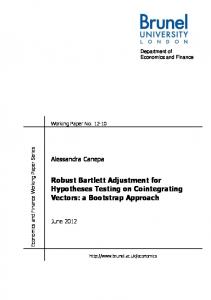
The two-hour plasma glucose data used in Fan et al. (2005) came from a study of diabetes conducted between 1984 and 1987 in Rancho Bernardo, California (Barrett-Connor, 1980a and 1980b). The data include 1025 men and 1301 women with a mean age of 71 (range 23-92). Figure 1 presents the distribution of plasma glucose concentrations for ages 20-49, 50-59, 60-69 and 70-79. Figure 2 presents the distribution of plasma glucose concentrations for males (ages 20-79) and females (ages 20-79). It can be seen from these figures that a bimodal mixture normal distribution may fit the blood glucose concentrations much better than a single mode normal distribution. The oldest age group (≥ 80 years) did

Bimodality of Plasma Glucose Distributions

485

not show statistically significant departure from a normal distribution and was hence not included in these figures.

0.15 0.00

0.00

0.05

0.10

0.10

0.15

Density of glucose concentration

0.20

Fmale: 20-79

0.05

Density of glucose concentration

Male: 20-79

0

5

10

15

20

25

30

0

5

10

2-hr glucose concentration (mmol/l)

15

20

25

30

2-hr glucose concentration (mmol/l)

Figure 2: Distributions of 2-hour plasma glucose concentrations for males and females. Solid smooth lines denote estimated densities and dashed smooth lines denote density curves of the two normal components.

A mixture normal distribution is often encountered in practice (McLachlan and Peel, 2000). A two-component normal mixture model may be written as p N (µ1 , σ12 ) + (1 − p) N (µ2 , σ22 ) ,

(1.1)

where 0 ≤ p ≤ 1 is the proportion of the first component, and µi and σi2 for i = 1, 2 denote the means and variances for the two components, respectively. When p = 0 or 1, the model in (1.1) reduces down to a one-component normal distribution. It is well known (e.g. Aitkin et al., 1981; McLachlan and Peel, 2000) that the likelihood ratio test (LRT) of H0 : one-component normal vs. Ha : twocomponent normal mixture model in (1.1) does not follow a chi-square test with degrees of freedom equal to the difference in the number of parameters between H0 and Ha . The null distribution of the LRT for mixture models is unknown. When the two normal components in the mixture distribution have equal variance, i.e., σ1 = σ2 , the p-value provided by the traditional LRT has been shown to be liberal (Thode et al., 1988) and an improved approximation by a chi-square distribution with 2.5 degrees of freedom has been suggested (Ning and Finch, 2000). When the two normal components in the mixture distribution have unequal variances, i.e., σ1 6= σ2 , simulation results have indicted that the limiting distribution is bounded by chi-square distributions with 4 and 6 degrees of freedom (McLachlan, 1987; Gutierrez et al., 1995).

486

Y. Yang, J. Fan, and S. May

Because the two components have unequal variances in the Rancho Bernardo data, the p-values in Fan et al. (2005) are based on a chi-square distribution with 6 degrees of freedom, which may be adequate or even a little conservative based on simulations conducted to investigate the distribution of the LRT for the Rancho Bernardo data (Yang, 2005). However, because the true null distribution of the likelihood ratio test for mixture models is unknown, it is possible that it may be data specific, i.e., the distribution of the LRT may depend on the parameter values under the null hypothesis as well as the sample size. Aitkin et al. (1981) attempted to compare values of the LRT, based on data simulated under the null hypothesis, to distributions of χ238 , χ239 , and χ276 , and concluded that none provided an adequate representation of their simulated LRT values. In this paper, we take a bootstrap based approach to studying the likelihood ratio test for mixture models. The rest of the paper is organized as follows. In section 2, we use a bootstrap approach to obtaining p-values for the LRTs for the two-hour plasma glucose concentrations data from the Rancho Bernardo Diabetes Study. In section 3, we evaluate the size and power of our approach through simulations. The paper is concluded in section 4 with a brief discussion. 2. A Bootstrap Approach to the Likelihood Ratio Test for Mixture Models The bootstrap significance test procedure consists of the comparison of the observed data to bootstrap samples generated according to the null hypothesis being tested. The outcome of the test is determined by the rank of the test statistic of the observed data relative to the values of the test statistic of the bootstrap samples from the null model which form the reference set (Hope, 1968; McLachlan, 1987). Let −2 log λ denote the value of the likelihood ratio test. Suppose we have generated K values of −2 log λ under the null hypothesis, and have one additional value of −2 log λ from the observed data. If the null hypothesis is true, then all (K + 1) values come from the null model. If there are i simulated values of −2 log λ greater than or equal to the observed value of −2 log λ, we estimate the p-value to be (i + 1)/(K + 1). For a specified significance level α, the value of K can be appropriately chosen. When K = 999, the p-value equals to (i + 1)/1000. For α = 0.05, the smallest value of K needed is 19 and the test is significant with a p-value of 0.05 only when i = 0, that is, when all 19 values of −2 log λ based on the bootstrap samples from the null model are smaller than the value of −2 log λ based on the original data.

Bimodality of Plasma Glucose Distributions

487

2.1 Algorithm for obtaining p-value of the LRT We will evaluate p-values of the likelihood ratio tests for the Rancho Bernardo data using both K = 999 and K = 19. The algorithm below summarizes the procedure for K = 999, for testing bimodality of plasma glucose distributions for each age and gender group. 1. Generate a bootstrap sample from the one-component normal distribution (H0 ) with the same mean and variance as estimated from the Rancho Bernardo data. The sample size of the generated data is also the same as that of each corresponding age and gender group. Calculate −2 log λ for the bootstrap sample. 2. Repeat step 1 by 999 times to obtain 999 simulated values of −2 log λ. 3. Calculate −2 log λ for the observed Rancho Bernardo data. 4. Count i (the total number of simulated values of −2 log λ greater than or equal to the observed value of −2 log λ). Calculate p = (i + 1)/1000. 2.2 The LRT applied to plasma glucose data The above algorithm was used to calculate the p-values for each age and gender group of the Rancho Bernardo data. As in Fan et al. (2005), the logarithm transformation was applied to the two-hour glucose concentration data to reduce skewness. The majority of the participants in the Rancho Bernardo Study were older than 60. We have only 84 people younger than 50, so all participants younger than 60 are combined in one age group. For the people older than 60, the grouping is based on 10- year intervals. The p-values from the test of normality indicated that the data were not normally distributed for all age groups except for participates older than 80. Therefore participants older than 80 were excluded from further study. The likelihood ratio test −2 log λ = −2{log(L0 ) − log(La )} was computed for each age and gender group, where L0 denotes the likelihood under H0 and La the likelihood under Ha . The value of log(L0 ) was obtained by substituting the maximum likelihood estimates (MLEs) of µ and σ into the log likelihood function for the one-component normal model. The two-component normal mixture model was fit using the expectation-maximization (E-M) algorithm. In order to reach the global rather than a local maximum, three starting points of the proportion p: 0.8, 0.85 and 0.90, were used to split the data into two subsets. Those starting points of p correspond to possible percentages of people with diabetes in the

488

Y. Yang, J. Fan, and S. May

population. The MLEs of the two means and two variances estimated from two subsets were used as our starting points of means and variances for the E-M algorithm. The largest log likelihood score from the three sets of initial values for the E-M algorithm was chosen as an estimate of log(La ). Table 1 shows the model fitting and hypothesis testing results for the logarithm transformed plasma glucose concentration by each age group, using K = 999. It indicates that the estimated mean log transformed glucose concentration increases from 4.70 to 4.92 as age increases under the one-component (unimodal) model. Under the two-component (bimodal) model, the estimated mean of the first mode increases from 4.66 to 4.87 while the mean of the second mode increases from 5.13 to 5.45 as age increases. The estimated percentage in the first mode is about 90% for each group. The estimated standard deviations of the first mode for the three age groups are similar with the value of 0.3 while the standard deviations in the second mode are about 0.4. The values of −2 log λ are large for all age groups. The p-values are very small with all values less than or equal to 0.003. Therefore the likelihood ratio test rejects the null hypothesis that the two-hour plasma glucose concentrations are from a one-component (unimodal) normal distribution. It indicates that a two-component (bimodal) normal mixture model fits the data better. Table 1: LRTs of log transformed blood glucose concentrations by age Unimodal Age 20-59 60-69 70-79

n

µ

σ

456 4.70 0.31 576 4.81 0.36 917 4.92 0.37

Bimodal µ1

σ1

µ2

σ2

p(%)

LRT

p-value

4.66 0.27 5.13 0.42 91.05 4.77 0.31 5.41 0.43 93.74 4.87 0.33 5.45 0.36 90.71

25.58 27.06 16.16

.001 .001 .003

The model fitting was repeated separately for men and women younger than 80. Table 2 shows the likelihood ratio test results by gender. The estimated means of blood glucose for men and women are virtually the same from the unimodal fitting and for the first mode of the two-component model. The estimated means of the second mode of the two-component model are slightly different, with 5.52 for males and 5.41 for females. The percentages in the first mode are 90.4% among males and 93.9% among females. The values of the LRTs in both groups are very large and the p-values for both groups are .001. These results indicate that a bimodal mixture normal model fits the data from each sex group better than a unimodal normal model. The analysis was repeated for K = 19. In each age and gender group, the observed value of −2 log λ is greater than all the simulated −2 log λ values, so the p-value in each group is equal to 0.05 (not shown in Tables 1 and 2). Hence, the

Bimodality of Plasma Glucose Distributions

489

same conclusion can be drawn. That is, the null hypothesis of a one-component normal model is rejected and a bimodal normal mixture model fits the plasma glucose data from Rancho Bernardo Study significantly better for each age and gender group. Table 2: LRTs of log transformed blood glucose concentrations by gender Unimodal Age

n

µ

σ

Male 836 4.84 0.39 Female 1113 4.84 0.34

Biomodal µ1

σ1

µ2

σ2

p(%)

LRT

p-value

4.76 0.33 5.52 0.30 90.43 4.80 0.30 5.41 0.39 93.90

27.54 39.78

.001 .001

3. Evaluation of Size and Power In order to evaluate the performance of the proposed procedure in Section 2 for testing between H0 : one-component normal model vs. Ha : two-component normal mixture model in (1.1), we next evaluate the size and power of the procedure. We will do the size and power calculations only for K = 19 since these calculations for K = 999 will require substantial computation time. 3.1 Algorithms for evaluating the size and power We will evaluate the size and power of the bootstrap based likelihood ratio test procedure for sample sizes n = 100, 250, 500, 750, and 1000. The algorithm for evaluating the size of the test is as follow. 1. Generate a sample of size n from the null hypothesis with mean equal to 5.0 and standard deviation equal to 0.4, similar to the mean and standard deviation values in Rancho Bernardo data. This sample is our “observed” data. 2. Calculate the likelihood ratio test −2 log λ for the “observed” data. 3. Calculate the p-value using the bootstrap test procedure with K = 19. That is, generate 19 bootstrap samples of size n from the normal distribution with mean and standard deviation equal to those estimated from the “observed” data. For each sample, calculate −2 log λ. The p-value is equal to 0.05 if the “observed” −2 log λ value from step 2 is greater than all 19 simulated values of −2 log λ. 4. Repeat steps 1-3 by 1000 times. Count the total number when the p-value is equal to 0.05. The size is the proportion of the times when the p-value is 0.05 out of 1000 repetitions.

490

Y. Yang, J. Fan, and S. May

The algorithm for evaluating the power is the same as that for evaluating the size except that, for power calculations, the “observed” data need to be generated from the alternative hypothesis instead of the null hypothesis. For the power evaluation, we replace step 1 in the previous algorithm by the following. Step 1 of the algorithm for evaluating power: 1. Generate a sample of size n from the alternative hypothesis with the proportion in the first component, two means and two standard deviations similar to those in Rancho Bernardo data. In particular, generate 90% of the sample from the normal distribution with mean 4.8 and standard deviation 0.3 denoted by N (4.8, 0.32 ), and 10% of the data from N (5.4, 0.42 ). This sample is our “observed” data. According to McLachlan (1987), the power of the LRT is related to the Mahalanobis distance ∆ = |µ1 − µ2 |/σ, where µ1 and µ2 are the two means of the two normal components in Ha and σ is the common standard deviation for the bimodal normal model. When the two means are chosen as 4.8 and 5.4 and two variances as 0.3 and 0.4, the Mahalanobis distance between the two components is close to 2. We evaluate the power also for ∆ = 1 and ∆ = 3. When ∆ = 1, we generate 90% of the “observed” data from the normal distribution N (4.8, 0.32 ), and 10% of the data from the normal distribution N (5.1, 0.42 ). For ∆ = 3, we generate 90% of the “observed” data from N (4.6, 0.32 ) and 10% of the data from N (5.5, 0.42 ). 3.2 Simulation results on size and power Table 3 shows the simulation results on size and power for sample sizes of n = 100, 250, 500, 750, and 1000. Note that each entry of the table is based on 1000 simulation runs. We see that the simulated size ranges from 0.047 to 0.059, all within 0.01 of the nominal level of 0.05, suggesting that the bootstrap based approach to testing mixture models preserves the type I error rate. The power of the bootstrap based likelihood ratio test increases when either the Mahalanobis distance or sample size increase. For Mahalanobis distance ∆ = 1, the power is as low as 0.09 for a sample size of 100. The power increases to 0.648 when the sample size increases to 1000. Therefore, it is hard to detect two components when the two means are only one standard deviation apart, unless the sample size is 1000 or more.

Bimodality of Plasma Glucose Distributions

491

Table 3: Simulation results on size and power Sample Size Size Power, ∆ = 1 Power, ∆ = 2 Power, ∆ = 3

100

250

500

750

1000

0.055 0.090 0.355 0.757

0.047 0.169 0.742 0.993

0.059 0.324 0.970 1.000

0.055 0.511 0.995 1.000

0.058 0.648 0.998 1.000

When the Mahalanobis distance increases to ∆ = 2, the power increases substantially at all sample sizes. The power is about 0.74 for a sample size of n=250. The power is greater than 0.97 when sample size is equal to or greater than 500. Therefore, the detection of two components is virtually guaranteed when the two means are about two standard deviations apart and the sample size is equal to or greater than 500. When the Mahalanobis distance increases to ∆ = 3, the power reaches 75.7% even at a small sample size of 100. The power is as high as 99.3% at a moderate sample size of 250. The power increases to 100% for sample sizes of 500 or greater. Thus we need only a sample size of 250 or greater to detect two components with a power of 99% and better when the two means are about three standard deviations apart. 4. Discussion The null distribution of the likelihood ratio test of unimodal normal model versus bimodal normal mixture model does not follow the chi-square distribution with degrees of freedom equal to the difference in the number of parameters between the two models. In this paper we take a bootstrap approach to gauging the likelihood of obtaining the observed data under the null hypothesis of a one-component normal model. The p-values from this approach indicate that a bimodal normal model fits the Rancho Bernardo plasma glucose data significantly better than a unimodal normal model. These results confirm that bimodality of blood glucose distributions exists in the Caucasian population (Fan et al., 2005). The size and power of the bootstrap based likelihood ratio test are evaluated in simulations for sample sizes of n = 100, 250, 500, 750 and 1000. The results indicate that the bootstrap based testing procedure has the correct size that is close to the nominal level of 0.05 and good power when the Mahalanobis distance is at least two and sample size is at least 250. The combinations of a Mahalanobis distance of 2 and sample size of 500, or a Mahalanobis distance of 3 and sample size of 250 provide a statistical power of at least 97% for detecting two components, when the level of significance is set at 0.05. For the Rancho Bernardo data, the Mahalanobis distance is about two. In

492

Y. Yang, J. Fan, and S. May

this case, the power is 97% or better if the sample size is at least 500. Thus for data similar to the Rancho Bernardo data, the bootstrap based likelihood ratio test has a high probability of detecting the two-component normal model. When the sample size decreases to 250, the power of the LRT decreases to 74% in our simulation study. This implies that bimodality may not be detected if one considers smaller subpopulations for the Rancho Bernardo data. An uneven mixing ratio (the proportion of the first mode p close to 1), a moderate Mahalanobis distance, and small sample size may have all contributed to the failure to detect bimodality of plasma glucose distributions in whites before the Rancho Bernardo Study. References Aitkin, M., Anderson, D., and Hinde, J. (1981). Statistical modeling of data on teaching styles. Journal of the Royal Statistical Society, Series A 144, 419-461. Barrett-Connor, E. (1980a). The prevalence of diabetes mellitus in an adult community as determined by history or fasting hyperglycemia. American Journal of Epidemiology 111, 705-712. Barrett-Connor, E. (1980b). Factors associated with the distribution of fasting plasma glucose in an adult community. American Journal of Epidemiology 112, 518-523. Fan, J. J., May, S. J., Zhou, Y., and Barrett-Connor, E. (2005). Bimodality of 2-h Plasma Glucose Distributions in Whites: The Rancho Bernardo Study. Diabetes Care 28, 1451-1456. Gutierrez, R. G., Caroll, R. J., Wang, N., Lee, G. H., and Taylor, B. H. (1995). Analysis of Tomato Root Initiation using a normal mixture distribution. Biometrics 51, 1461-1468. Harris, M. I., Flegal, K. M., Cowie, C. C., Eberhardt, M. S., Goldstein, D. E., Little, R. R., Wiedmeyer, H. -M., and Byrd-Holt, D. D. (1998). Prevalence of diabetes, impaired fasting glucose, and impaired glucose tolerance in U. S. Adults: The Third National Health and Nutrition Examination Survey, 1988-94. Diabetes Care 21, 518-524. Hope, A. C. A. (1968). A simplified Monte Carlo significance test procedure. Journal of the Royal Statistical Society, Series B 30, 582-598. McLachlan, G. J. (1987). On Bootstrapping the Likelihood Ratio Test Statistic for the Number of Components in a Normal Mixture. Applied Statistics 36, 318-324. McLachlan, G. and Peel, D. (2000). Finite Mixture Models. John Wiley & Sons, New York. Ning, Y. M. and Finch, S. J. (2000). The null distribution of the likelihood ratio test for a mixture of two normals after a restricted Box-Cox transformation. Communications in Statistics-Simulation and Computation 29, 449-461.

Bimodality of Plasma Glucose Distributions

493

Raper, L. R., Taylor, R., Zimmet, P., Milne, B., and Balkau, B. (1984). Bimodality in glucose tolerance distributions in the urban polynesian population of Western Samoa. Diabetes Research 1, 1-8. Rosenthal, M., McMahan, C. A., Stern, M. P., Eifler, C. W., Haffner, S. M., Hazuda, H. P., and Franco, L. J. (1985). Evidence of bimodality of two hour plasma glucose concentrations in Mexican Americans: results from the San Antonio Heart study. Journal of Chronic Diseases 38, 5-16. Rushforth, N. B., Bennett, P. H., Steinberg, A. G., Burch, T. A., and Miller, M. (1971). Diabetes in the Pima Indians: Evidence of bimodality in glucose tolerance distributions. Diabetes 20, 756-765. Steinberg, A. G., Rushforth, N. B., Bennett, P. H., Burch, T. A., and Miller, M. (1970). On the genetics of diabetes mellitus: Nobel Symposium 13. In The Pathogenesis of Diabetes Mellitus. Cerasi, E. and Luft, R., Eds. New York, Wiley, p. 237-264. Thode, H. C., Finch, S. J., and Mendell, N. R. (1988). Simulated percentage points for the null distribution of the likelihood ratio test for a mixture of two normals. Biometrics 44, 1195-1201. Yang, Y. (2005). The likelihood ratio test for a mixture of two normals: with application to the bimodality of plasma glucose. San Diego State University thesis. Zimmet, P. and Whitehouse, S. (1978). Bimodality of fasting and two-hour glucose tolerance distributions in a Micronesian population. Diabetes 27, 793-800. Received October 9, 2008; accepted October 30, 2008.

Ying Yang Biostatistics Division Department of Public Health Sciences University of California at Davis Davis, CA 95616, USA [email protected] Juanjuan Fan Department of Mathematics and Statistics San Diego State University San Diego, CA 92182, USA [email protected] Susanne May Department of Biostatistics University of Washington Seattle, WA 98195, USA [email protected]