A brief introduction to nonperturbative calculations in light-front QED

A brief introduction to nonperturbative calculations in light-front QEDa Sophia S. Chabysheva Department of Physics University of Minnesota-Duluth Duluth, Minnesota 55812

arXiv:1010.0214v1 [hep-ph] 1 Oct 2010

(Dated: October 4, 2010)

Abstract A nonperturbative method for the solution of quantum field theories is described in the context of quantum electrodynamics and applied to the calculation of the electron’s anomalous magnetic moment. The method is based on light-front quantization and Pauli–Villars regularization. The application to light-front QED is intended as a test of the methods in a gauge theory, as a precursor to possible methods for the nonperturbative solution of quantum chromodynamics. The electron state is truncated to include at most two photons and no positrons in the Fock basis, and the wave functions of the dressed state are used to compute the electrons’s anomalous magnetic moment. A choice of regularization that preserves the chiral symmetry of the massless limit is critical for the success of the calculation. PACS numbers: 12.38.Lg, 11.15.Tk, 11.10.Gh, 11.10.Ef

a

Contributed to the proceedings of QCD@Work 2010, the international workshop on QCD Theory and Experiment, Martina Franca, Italy, June 20-23, 2010.

1

I.

INTRODUCTION

The purpose of this work is to explore a nonperturbative method that can be used to solve for the bound states of quantum field theories, in particular QCD. The problem is notoriously difficult, and there are only a few approaches. These include lattice gauge theory [1], the transverse lattice [2], Dyson–Schwinger equations [3], Bethe–Salpeter equation, similarity transformations combined with construction of effective fields [4], light-front Hamiltonians with either standard [5] or sector-dependent parameterizations [6–8]. We use the light-front Hamiltonian approach with Pauli–Villars (PV) [9] regularizaton and standard parameterization, where the bare parameters of the Lagrangian do not depend on the Fock sector. This means that we use Fock states – the states with definite particle number and definite momentum for each particle – as the basis for the expansion of eigenstates. The coefficients in such an expansion are the wave functions for each possible set of constituent particles. These functions describe the distribution of internal momentum among the constituents. Such an expansion is infinite, and we truncate the expansion to have a calculation of finite size. The wave functions are determined by a coupled set of integral equations which are obtained from the bound-state eigenvalue problem of the theory. Each bound state is an eigenstate of the field-theoretic Hamiltonian, and projections of this eigenproblem onto individual Fock states yields these coupled equations. Each equation is a relativistic analog of the momentum-space Schr¨odinger equation, but with terms that couple the equation to other wave functions that represent different sets of constituents, perhaps one gluon more or less or a quark-antiquark pair in place of a gluon or vice-versa. The solution of such equations, in general, requires numerical techniques. The equations are converted to a matrix eigenvalue problem by some discretization of the integrals or by a function expansion for the wave functions. The matrix is usually large and not diagonalizable by standard techniques; instead, one or some of the eigenvalues and eigenvectors are extracted by the iterative Lanczos process. The eigenvector of the matrix yields the wave functions, and from these can be calculated the properties of the eigenstate, by considering expectation values of physical observables. We work with light-cone coordinates [10, 11], chosen in order to have well-defined Fockstate expansions and a simple vacuum. The time coordinate is x+ = t + z and the space coordinates are x = (x− , ~x⊥ ), with x− ≡ t − z and ~x⊥ = (x, y). The light-cone energy is p− = E − pz , and the three-momentum is p = (p+ , ~p⊥ ), with p+ ≡ E + pz and p~⊥ = (px , py ). m2 +p2

The mass-shell condition p2 = m2 becomes p− = p+ ⊥ . The simple vacuum follows from p the positivity of the plus component of the momentum: p+ ≡ m2 + p2z + p2⊥ + pz > 0. To regulate a theory, we use the Pauli–Villars technique [9]. The basic idea is to subtract from each integral a contribution of the same form but of a PV particle with a much larger mass. This can be done by adding negative metric particles to the Lagrangian. For example, for free scalars a Lagrangian of the form     1 1 2 2 1 2 2 1 2 2 L = (∂µ φ0 ) − µ0 φ0 − (∂µ φ1 ) − µ1 φ1 (1.1) 2 2 2 2 generates a contribution from an internal line of a Feynman diagram in the form  Z  1 1 d4 p, − p2 − µ20 p2 − µ21 2

(1.2)

=

+

+

+

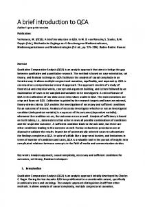
FIG. 1. The Fock-state expansion of the dressed-electron eigenstate.

which has the necessary subtraction. A particular advantage of PV regularization is preservation of at least some symmetries; in particular, it is automatically relativistically covariant. II.

APPLICATION TO QED

The method is not mature enough to apply to QCD, so as a test in a gauge theory, we consider light-front QED and specifically the eigenstate of the dressed electron and its anomalous moment [12–15]. From the PV regulated light-front QED Lagrangian, we 2 construct the Hamiltonian P − and solve the mass eigenvalue problem P − |P i = M |P i in P+ the approximation that the electron eigenstate is a truncated Fock-state expansion with at most two photons and no positrons [15]. From this approximate eigenstate, we compute the anomalous magnetic moment from the spin-flip matrix element of the electromagnetic current J + [16]. Schematically, the electron Fock-state expansion can be written Z Z Z Z (2.1) |electroni = ψe |ei + ψeγ |eγi + ψeγγ |eγγi + ψeee+ |ee+ i + · · · This is represented graphically in Fig. 1 It satisfies the eigenvalue problem HLC |electroni = (K + VQED ) |electroni = M 2 |electron,

(2.2)

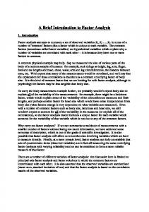
where VQED is the potential-energy operator, represented graphically in Fig. 2. The projec-

VQED

=

+

+

+

+

FIG. 2. The potential-energy operator of light-front QED in a graphical representation.

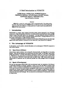
tions of this eigenvalue problem onto each individual Fock state produces coupled equations for the Fock-state wave functions, which are schematically represented in Fig. 3. The first graphical equation in Fig. 3 is a projection onto the one-electron Fock state, which can be written as Z 2 m0 ψe + dk γ Veγ→e (k γ )ψeγ (k γ ) = M 2 ψe . (2.3) 3

×

= M2

+

× = M2

+

+ × × ×

= M2

+

×

FIG. 3. A graphical representation of the coupled equations for the Fock-state wave functions of the dressed electron eigenstate.

It includes absorption of the photon from the one-electron/one-photon state. The second equation can be expressed as Z X m2 + k 2 i i ψeγ + dk γ Veγ→e (k γ )ψeγγ (k γ ) = M 2 ψeγ . (2.4) + + ki /p i This includes photon emission by the bare electron and photon absorption from the oneelectron/two-photon state. The third equation is the analogous one for the three-body sector. The first and third equations of the coupled system can be solved for the bare-electron amplitudes and one-electron/two-photon wave functions, respectively, in terms of the oneelectron/one-photon wave functions. Substitution of these solutions into the second integral equation yields a reduced integral eigenvalue problem in the one-electron/one-photon sector. A diagrammatic representation is given in Fig. 4. Solution of the resulting integral equations yields α as a function of m0 and the PV masses. Then for given values of PV masses, we can seek the value of m0 for which α takes the standard physical value e2 /4π. The equations must first be solved for M = 0, with the coupling strength parameters adjusted to yield m0 = 0 [15]. The solution of the integral equations requires numerical techniques [15]. The integrals are discretized via quadrature rules, and the equations are thereby converted to a matrix eigenvalue problem, which is solved by iteration. 1

III.

RESULTS

From the solutions to the eigenvalue problems, we compute the anomalous moment at fixed PV masses and fixed numerical resolution. We then study the behavior first as a function of the numerical resolution, which requires extrapolation, and then as a function of PV masses. The numerical resolution is marked by two parameters, K and N⊥ , which control the number of quadrature points used in the longitudinal and transverse directions. The numerical convergence and extrapolation are illustrated in [15]. 4

×

+

+

×

+

= M2 FIG. 4. Diagrammatic representation of effective integral equation in the one-electron/one-photon sector.The first term represents the kinetic energy; the second and third, the two time orderings of photon absorption and emission; and the fourth, the self-energy contribution.

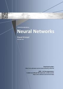
The results of the extrapolations are plotted in Fig. 5. Each value is close to the standard Schwinger result of α/2π and independent of µ1 , to within numerical error. The results with only the two-photon self-energy contribution are actually better than the full two-photon results. This discrepancy should be due to the absence of electron-positron contributions, which are of the same order in α as the two-photon contributions; without the electron-positron contributions, we lack the cancellations that typically take place between contributions of the same order.

2 If we retain only the self-energy contributions from the two-photon intermediate states, the equations for the two-body wave functions become much simpler, and the coupled integral equations can be reduced to the one-electron sector. There, they can be solved analytically, except for the calculation of certain integrals [14]. We see that the inclusion of the self-energy contribution is a significant improvement over the one-photon truncation. Thus, we expect that inclusion of the three-photon self-energy will improve the two-photon results.

Figure 5 also includes results obtained for the two-photon truncation when only the oneloop chiral constraint is satisfied. Without the full nonperturbative constraint, the results are very sensitive to the PV photon mass µ1 . This behavior repeats the pattern observed in [12] for a one-photon truncation without the corresponding one-loop constraint. The resulting µ1 dependence is illustrated in Fig. 2 of [12]. Thus, a successful calculation requires that the symmetry of the chiral limit be maintained. 5

1.2

(2π/α) ae

1.0 0.8 0.6 one-photon truncation with self-energy two-photon truncation insufficient, one-loop constraint

0.4 0.2 0

100

200

300

400

500

µ1/me FIG. 5. The anomalous moment of the electron in units of the Schwinger term √ (α/2π) plotted versus the PV photon mass, µ1 , with the second PV photon mass, µ2 , set to 2µ1 and the PV electron mass m1 equal to 2 · 104 me . The solid squares are the result of the full two-photon truncation with the correct, nonperturbative chiral constraint [15]. The open squares come from use of a perturbative, one-loop constraint. Results for the one-photon truncation [12] (solid line) and the one-photon truncation with the two-photon self-energy contribution [14] (filled circles) are included for comparison. The resolutions used for the two-photon results are K = 50 to 150, combined with extrapolation to K = ∞, and N⊥ = 20. ACKNOWLEDGMENTS

The work reported here was done in collaboration with J.R. Hiller and supported in part by the Minnesota Supercomputing Institute.

[1] For reviews of lattice theory, see M. Creutz, L. Jacobs, and C. Rebbi, Phys. Rep. 95, 201 (1983); J.B. Kogut, Rev. Mod. Phys. 55, 775 (1983); I. Montvay, ibid. 59, 263 (1987); A.S. Kronfeld and P.B. Mackenzie, Ann. Rev. Nucl. Part. Sci. 43, 793 (1993); J.W. Negele, Nucl. Phys. A553, 47c (1993); K.G. Wilson, Nucl. Phys. B (Proc. Suppl.) 140, 3 (2005); J.M. Zanotti, PoS LAT2008, 007 (2008). For recent discussions of meson properties and charm physics, see for example C. McNeile, and C. Michael [UKQCD Collaboration], Phys. Rev. D 74, 014508 (2006); I. Allison et al. [HPQCD Collaboration], Phys. Rev. D 78, 054513 (2008). [2] M. Burkardt, and S. Dalley, Prog. Part. Nucl. Phys. 48, 317 (2002) and references therein; S. Dalley, and B. van de Sande, Phys. Rev. D 67, 114507 (2003); D. Chakrabarti, A.K. De, and A. Harindranath, Phys. Rev. D 67, 076004 (2003); M. Harada, and S. Pinsky, Phys. Lett. B

6

[3]

[4]

[5]

[6] [7] [8] [9] [10] [11] [12] [13] [14] [15] [16]

567, 277 (2003); S. Dalley, and B. van de Sande, Phys. Rev. Lett. 95, 162001 (2005); J. Bratt, S. Dalley, B. van de Sande, and E. M. Watson, Phys. Rev. D 70, 114502 (2004). For work on a complete light-cone lattice, see C. Destri, and H.J. de Vega, Nucl. Phys. B290, 363 (1987); D. Mustaki, Phys. Rev. D 38, 1260 (1988). C.D. Roberts, and A.G. Williams, Prog. Part. Nucl. Phys. 33, 477 (1994); P. Maris, and C.D. Roberts, Int. J. Mod. Phys. E12, 297 (2003); P.C. Tandy, Nucl. Phys. B (Proc. Suppl.) 141, 9 (2005). S. D. Glazek, and R. J. Perry, Phys. Rev. D 78, 045011 (2008); S.D. Glazek, and J. Mlynik, Phys. Rev. D 74, 105015 (2006); S.D. Glazek, Phys. Rev. D 69, 065002 (2004); S.D. Glazek, and J. Mlynik, Phys. Rev. D 67, 045001 (2003); S.D. Glazek, and M. Wieckowski, Phys. Rev. D 66, 016001 (2002). S.J. Brodsky, J.R. Hiller, and G. McCartor, Phys. Rev. D 58, 025005 (1998); 60, 054506 (1999); 64, 114023 (2001); Ann. Phys. 296, 406 (2002); 305, 266 (2003); 321, 1240 (2006); S.J. Brodsky, V.A. Franke, J.R. Hiller, G. McCartor, S.A. Paston, and E.V. Prokhvatilov, Nucl. Phys. B 703, 333 (2004). R.J. Perry, A. Harindranath, and K.G. Wilson, Phys. Rev. Lett. 65, 2959 (1990); R.J. Perry, and A. Harindranath, Phys. Rev. D 43, 4051 (1991). V. A. Karmanov, J. F. Mathiot, and A. V. Smirnov, Phys. Rev. D 77, 085028 (2008); arXiv:1006.5640 [hep-th]. J.P. Vary et al., Phys. Rev. C 81, 035205 (2010). W. Pauli and F. Villars, Rev. Mod. Phys. 21, 434 (1949). P.A.M. Dirac, Rev. Mod. Phys. 21, 392 (1949). For reviews of light-cone quantization, see M. Burkardt, Adv. Nucl. Phys. 23, 1 (2002); S.J. Brodsky, H.-C. Pauli, and S.S. Pinsky, Phys. Rep. 301, 299 (1998). S.S. Chabysheva, and J.R. Hiller, Phys. Rev. D 79, 114017 (2009). S.S. Chabysheva, A nonperturbative calculation of the electron’s anomalous magnetic moment, Ph.D. thesis, Southern Methodist University, ProQuest Dissertations & Theses, 3369009, 2009. S.S. Chabysheva, and J.R. Hiller, Ann. Phys. 325, 2435 (2010). S.S. Chabysheva, and J.R. Hiller, Phys. Rev. D 81, 074030 (2010). S.J. Brodsky and S.D. Drell, Phys. Rev. D 22, 2236 (1980).

7