MFPS 2010
A categorical setting for lower complexity Robin Cockett1 ,3 , Brian F. Redmond2 ,4 Department of Computer Science University of Calgary Calgary, Canada
Abstract A polarized strong category consists of a cartesian category, X, and a category Y, together with a module M : X × Y − → Y equipped with a strong composition and identities. These categories can be used to provide an abstract setting for investigating computational setting with complexity below primitive recursive. This paper develops the theory of polarized strong categories, explains how they relate to the theory of fibrations, and provides a concrete example which illustrates their applicability to these lower complexity systems of computation. Keywords: Polarized categories, fibrations, recursion principles, complexity.
1
Introduction
It is well-known that having a (strong) natural number object in a monoidal category immediately delivers all primitive recursive functions [19]. Therefore, to obtain settings which realize lower complexities something quite drastic has to be done. An attractive feature, however, of a natural number object is that, as an initial data type, it arrives packaged with a universal property which enforces certain basic equalities on the maps involving that type. In the initial models of a doctrine involving such a type, these equalities become the basis for generating all the equality judgements. As computation is often viewed as 1 2 3 4
Partially supported by NSERC, Canada. Partially supported by NSERC, Canada, and PIMS. Email:
[email protected] Email:
[email protected] This paper is electronically published in Electronic Notes in Theoretical Computer Science URL: www.elsevier.nl/locate/entcs
Cockett, Redmond
arising from initial settings, this native notion of equality is of considerable interest. In dealing with settings which are below primitive recursive our interest is not merely in the presence or absence of maps but also in the notion of equality which they support. Therefore, we would like data types, even in these settings, to deliver a universal property and whence a native notion of equality. This paper describes for lower complexity settings how initial inductive data types – together with their corresponding universal property – can be supplied by moving to polarized strong categories. We illustrate this with a simple semantic setting, which we develop in some detail, which uses R-sized sets 5 and polynomially bounded maps. The significance of this example is that its arithmetic power is strictly less than primitive recursive (because of the explicit polynomial bound) although it is at least as powerful as PSPACE (as only the size of the output is controlled). The example, of course, opens the question of whether the full system we describe can capture Polynomial Time (PTIME) and Polynomial Space (PSPACE) computations. For discussion of these matters see the conclusion of this paper and the report [20] in which a much fuller type theory is discussed in support of a PTIME programming language called Pola which is currently being developed by Mike Burrell [3]. The focus of the current paper is on the categorical doctrines 6 which can be used for modeling the proof theories of these lower complexity settings. The nucleus from which this paper grew was the realization that the system of Bellantoni and Cook [2] for describing PTIME had an immediate interpretation as a proof theory for a polarized logic. Polarities were introduced by Girard [6] to classify the behavior of the logical connectives in his “constructive” classical logic LC – his idea was directly related to Andreoli’s notion of focussing [1]. Olivier Laurent [14] further developed these ideas and quickly realized that there was a compelling connection to games [15]: these and further references to related developments are described in [7]. The general categorical proof theory for polarized logics and games is described in [4] and uses the notion of a polarized category. A polarized category is simply a module 7 , however, viewed as a categorical structure in its own right. Polarization is produced by the separation beween the category which 5
These play a similar role to the “length spaces” of [9]. The program of expressing complexity classes categorically is not new. Notable was Jim Otto’s [18] pioneering work. The first author would particularly like to acknowledge his conversations with Jim – they were formative in this work. 7 A module M : X − → Y is variously called a profunctor, a distributor, a bi module: it is equivalently a functor M : Xop × Y − → Set or a “bipartite” category consisting of the categories X and Y and in addition “cross maps” running from the objects of X to objects of Y – but not in the reverse direction. 6
2
Cockett, Redmond
is the domain of the module (the “opponent” world) and the category which is the codomain (the “player world”). While Bellantoni and Cook used the terms “ordinary” and “safe” (respectively) for the two worlds of computation – rather than the game theory inspired terminology used here – it was clear that they were employing the technique of polarizing to achieve separation for computation. Bellantoni and Cook’s system of safe recursion, which only considered binary natural numbers, was a simplification of a slightly earlier system developed by Leivant [16] which had general inductive data types and infinitely many tiers (although two sufficed). Both these systems allowed duplication in their “safe” worlds and focused on controlling the recursion. The categorical doctrine we present, however, uses a further crucial idea introduced by Hofmann [10]: he realized that it was advantageous to assume that the player (or safe) world is affine – so one cannot duplicate data. This allows one to restrict the “safe” or player world to constant time computations (in context). The intuition is then that “iterating” (parameterized) constant time computations keeps one within polynomial time. Of course, a categorical doctrine which demands that the player world be affine is quite happy to accept as a model a system which has duplication as well. Thus, the above mentioned systems are not ruled out from being a model of a categorical doctrine which assumes an affine player world. However, Hofmann’s reason for insisting on an affine world was more fundamental: he had observed that one could not allow certain reasonable patterns of recursion over trees – such as counting their leaves (see section 5.3) – at the same time as allowing their duplication. This is because, with duplication, one can easily construct an exponential size tree by simply repeatedly adding a root node whose children are duplicates of the tree constructed so far. Counting the leaves of such a tree takes one outside PTIME. Leivant’s system evaded this problem by supporting a recursion principle which did not permit one to count the leaves of a tree. There is, thus, a trade-off between the power of the recursion principle and allowing duplication in the player world. In the main system presented here, the player world is higher-order and this commits us to a powerful recursion principle and, whence, to limiting duplication. Of course, we could equally well have taken the other approach: allowing duplication and limiting the recursion principle. However, the power of the recursion principle significantly impacts expressiveness and this severely limits the utility of systems with restrictive recursion principles. Thus, here we have chosen the other direction, namely to promote the use of a more powerful recursion principle, as we feel it holds more promise.
3
Cockett, Redmond
Acknowledgements We thank Geoff Cruttwell for reading an early draft of the paper and for making many useful suggestions and observations.
2
The basic categorical setting
The basic categorical framework of this paper consists of a cartesian category X, a category Y, and a module connecting X × Y − → Y creating a polarized category [4] which is, in addition strong. The category X will referred to as the opponent category (or opponent world) and the category Y is referred to as the player category (or player world) while the module maps are referred to as cross maps. Polarized strong categories are closely related to certain fibrations (over the opponent world). This provides an alternative and compelling perspective on these setting which we shall wish to exploit. This section, therefore, develops the relationship to fibrations and also introduces R-sized sets which we shall use as a running example to illustrate the theory. 2.1 Polarized strong categories A polarized strong category consists of a cartesian category 8 X (the opponent world), and a category Y (the player world), and a module M : M :X×Y− →Y equipped with a “strong” composition and “strong” identities for the module maps: f g (X1 , Y1 ) −−→ Y2 (X2 , Y2 ) −→ Y3 f; g
(X1 × X2 , Y1 ) −−−→ Y3
i
(1, Y ) −−Y→ Y
which satisfy: •
Strong identities are natural: iY y = (1, y)iY 0 , for any y : Y − → Y 0 in Y;
•
The strong composition preserves the basic module structure: (f ; f 0 )y = f ; (f 0 y), (x1 × x2 , y)(f1 ; f2 ) = ((x1 , y)f1 ); (x2 , 1)f2 , and (1 × x, 1)((f y); f 0 ) = f ; (x, y)f 0 ;
•
(π1 , 1)f = iY ; f : (1 × X, Y ) − → Y 0 and (π0 , 1)f = f ; iY 0 : (X × 1, Y ) − → Y 0;
•
(a× , 1)((f1 ; f2 ); f3 ) = f1 ; (f2 ; f3 ) : (X1 × (X2 × X3 ), Y ) − → Y 0.
In order to demonstate the connection to fibrations we shall want to consider a fixed opponent world and a varying player world and to facilitate this 8
Here this means having finite products. In fact, having a tensor also suffices for the basic strong composition structure; see [23].
4
Cockett, Redmond
we shall refer to a polarized strong category with opponent world X as an X-strong category. An X-strong functor F : Y − → Y0 between X-strong categories will then be an ordinary functor F : Y − → Y0 and a morphism, also labeled F , on cross maps such that: f
(X, Y ) −−→ Y 0 F (f )
(X, F (Y )) −−−−→ F (Y 0 ) which preserve the basic module structure (x, F (y))F (h)F (y 0 ) = F ((x, y)hy 0 ) and preserves the strong composition and identities: •
F (iY ) = iF (Y )
•
F (f1 ; f2 ) = F (f1 ); F (f2 )
Clearly the composite of two X-strong functors is again an X-strong functor. An X-strong transformation between strong functors is an ordinary transformation between the ordinary functors α : F − → F 0 such that for cross maps 0 h we have (1, α)F (h) = F (h)α. We now have: Proposition 2.1 X-strong categories, functors, and transformations form a 2-category, written Str(X). 2.2 Fibrational interpretation e − Given an X-strong category Y a fibration p : Y → X can be constructed 9 , e of this fibracalled the bundle fibration bun(Y), where the total category Y tion is defined as follows: Objects: pairs of objects (X, Y ) ∈ X × Y; Maps: A map from (X1 , Y1 ) to (X2 , Y2 ) is a pair (x, h), where x : X1 − → X2 in X and h : (X1 , Y1 ) − → Y2 is a module map; Composition: let (x, h) : (X1 , Y1 ) − → (X2 , Y2 ) and (x0 , h0 ) : (X2 , Y2 ) − → (X3 , Y3 ); then composition is defined by (xx0 , (∆, 1)(h; (x, 1)h0 )) : (X1 , Y1 ) − → (X3 , Y3 ); Identities: (1X , (!X , 1)iY ) : (X, Y ) → (X, Y ). e is a category and moreover gives rise to a It is not hard to check that Y fibration: e − Proposition 2.2 The bun(Y) given by the projection functor p : Y → X defined by p(X, Y ) = X and p(x, h) = x is a fibration over X with a cleavage. 9
This is not the usual Grothendieck fibration from the module but uses the extra composition ‘;’ of an X-strong category in an essential way.
5
Cockett, Redmond
Proof. For each map x : X − → X 0 and object (X 0 , Y 0 ) over X 0 , the cartesian → (X 0 , Y 0 ). Indeed, f is lifting is defined as f = (x, (!X , 1)iY 0 ) : (X, Y 0 ) − cartesian over x as p(f ) = x and given g = (z, h) : (Z1 , Z2 ) − → (X 0 , Y 0 ) such that z factors as x0 x, there exists a bundle map m = (x0 , h) : (Z1 , Z2 ) − → (X, Y 0 ) such that p(m) = x0 and: mf = = = = = =
(x0 , h)(x, (!X , 1)iY 0 ) (x0 x, (∆, 1)(h; (x0 , 1)(!X , 1)iY 0 )) (z, (∆, 1)(h; (!Z1 , 1)iY 0 )) (z, (∆, 1)(1×!Z1 , 1)(h; iY 0 )) (z, (∆, 1)(1×!Z1 , 1)(π0 , 1)h) (z, h) = g
Moreover, if m0 = (x00 , h0 ) also satisfies these conditions, then x00 = p(m0 ) = x0 and m0 f = (z, h0 ) = g = (z, h), so h = h0 and m is unique. 2 Proposition 2.3 This assignment extends to a 2-functor bun : Str(X) − → CFib(X) which, moreover, preserves products. Proof. The preservation of products is immediate from the construction. An X-strong functor F extends to a cartesian functor Fe on the fibration as follows: Fe(X, Y ) = (X, F (Y )) Fe(x, h) = (x, F (h)) This preserves the cleavage as Fe(x, (!X , 1)iY ) (x, (!X , 1)iF (Y ) ) and is a functor as:
=
(x, F ((!X , 1)iY ))
Fe(1X , iY ) = (1X , F ((!X , 1Y )iY )) = (1X , (!X , F (1Y ))F (iY )) = (1X , (!X , 1F (Y ) )iF (Y ) ) and: Fe(x, h); Fe(x0 , h0 ) = = = = = =
(x, F (h))(x0 , F (h0 )) (xx0 , (∆, 1)(F (h); (x, 1)F (h0 ))) (xx0 , (∆, 1)(F (h); F ((x, 1)h0 ))) (xx0 , (∆, 1)(F (h; (x, 1)h0 ))) (xx0 , F ((∆, 1)(h; (x, 1)h0 ))) Fe((x, h)(x0 , h0 )) 6
=
Cockett, Redmond
The cartesian lifting of a map x : X − → X 0 in X is (x, (!X , 1)iY ) : (X, Y ) − → (X 0 , Y ). This map is preserved as Fe((x, (!X , 1Y )iY )) = (x, F ((!X , 1Y )iY )) = (x, (!X , 1F (Y ) )iF (Y ) ). Therefore Fe is a cartesian functor. A X-strong natural transformation α : F − → G extends to a cartesian e as follows: the components of the natural natural transformation α e : Fe − →G transformation are (1X , (!X , 1)αY ) : (X, F (Y )) − → (X, G(Y )). It is easy to check that this in fact defines a cartesian natural transformation. 2
Given any cartesian category X then X, itself, can be regarded as a Xstrong category by letting the cross maps be:
h
X1 × X −−→ X2 h
(X, X1 ) −−→ X2
This makes these cross maps “maps in context”. Note that this makes f ; g = a× (f × 1)g. A X-strong functor F then becomes a strong functor in the usual sense [13,5,23]. We now show that there is a functor in the reverse direction: that is, given any fibration (here we consider fibrations with a cleavage) over a cartesian category X the fiber over 1 naturally forms an X-strong category.
Proposition 2.4 There is a 2-functor pol : CFib(X) − → Str(X).
Proof. (Sketch) Let p : Y − → X be a fibration with cleavage. Then we may build an X-strong category on the fiber over 1, p−1 (1), where one defines a cross map of the form (X, Y ) − → Y 0 as a map !∗X (Y ) − → Y 0 in Y. The strong identity maps are the identity maps in p−1 (1). The strong composition of f
g
(X1 , Y ) =!∗X1 (Y ) −−→ Y 0 and (X2 , Y 0 ) =!∗X2 (Y 0 ) −→ Y 00 is given by lifting the fe
first map to the map (X1 × X2 , Y ) −−→ (X2 , Y 0 ) (as illustrated below) and 7
Cockett, Redmond
composing with g: (X1 × X2 , Y ) YYY
YYYYYY YYYYYY!∗ YYYYYY YYYYYY π f0 YYYYYY ' ,/ (X1 , Y ) UU (1, Y ) ∗ UUUU ! UUUU UUUU UUUU f fe UU* . (X , Y 0 ) / (1, Y 0 ) ∗ 2 LLL ! LLL g LLLL %
(1, Y 00 )
X1 × XP2PYYYYYY
YYYYYY PPP YYYYY!Y PPP YYYYYY π0 PPP YYYYYY PP' YYYYYY YY/, X1 ! qq8 1 q q q !q π1 qqq q q q / X2
A morphism of fibrations F : (p : Y − → X) − → (q : Y0 − → X) consists of 0 a functor F : Y − → Y such that p = F ; q which preserves the cleavage. The restriction to the fiber over 1 then defines an X strong functor between the induced X-strong categories. Similarly a natural transformation between a morphism of fibrations induces an X-strong transformation. 2 Proposition 2.5 The above functors forms an adjunction bun a pol : Str(X) − → CFib(X). Proof. (Sketch) The unit of the adjunction carries Y to the fiber over 1 in bun(Y): (1, Y )
Y η:Y− → pol(bun(Y)); ²
f
7→
Y0
²
(11 ,iY f )
(1, Y 0 )
We need to show the following universal property: η
/ pol(bun(Y)) QQQ QQQ Q pol(H ] ) H QQQQ ( ²
Y QQQQ
pol(A)
To do this we indicate how H ] is defined on (x, f ) ∈ bun(Y) using the lifting property (dotted maps) of the fibration A and the definition (X, A) :=!∗X (Y ) ∈ 8
Cockett, Redmond
p−1 (X) as above: H ] (x,f )
/ (X, Y 0 ) /, (X 0 , Y 0 ) ] s JJ (1,x) JJ ss JJ ss∗ s s H(f ) JJ sy s ! % 0 (1, Y ) l ∗
(X, Y J)
]) H(f
!
x
/X rr LLL r r ! r LL rrr ! LLL L& rx rrr j
X LLL
x
1
1
/+ X 0
!
This is clearly unique as the liftings are unique. To show this is a Galois adjunction it suffices to check that bun(η) is an isomorphism: however, this morphism of fibration is determined by its effect on the fiber over 1 and these fibers are essentially the same category. 2 The fact that there is a Galois adjunction between Str(X) and CFib(X) means that one can identify a common full subcategory: the subcatgory of CFib(X) corresponds to “bundle fibrations” while the full subcategory of Str(X) corresponds more prosaically to the X-strong categories in which Y is already the fibre over 1 in bun(Y). 2.3 The category of R-sized-sets Let R = (R, +, ·, 0, 1, ≤) be a size rig: that is an ordered (commutative) rig R with bottom element 0 (that is 0 ≤ r for all r ∈ R), and order-preserving operations. The canonical rig we have in mind is the natural numbers N (but R≥0 or Q≥0 will also do). The category of R-sized sets with polynomially bounded maps, denoted R-Setpoly , is constructed as follows: Objects: an object is a function α : A − → R. We may think of this as a set A, each of whose elements is assigned an abstract size (i.e. an element of R). These are called R-sized sets; Maps: A map from α : A − → R to β : B − → R is a function f : A − → B such that there exists a polynomial p ∈ R[x] satisfying: for all a ∈ A, β(f (a)) ≤ p(α(a)). In this case we say that p is a bound for f ; Composition: The usual function composition. The composite is bounded by substitution of polynomials. Identities are the identity functions with identity polynomial bounds. It is clear that this forms a category. It is furthermore a cartesian category. 9
Cockett, Redmond
The product of R-sized sets α : A − → R and β : B − → R is the sized set A×B − → R; (a, b) 7→ α(a) + β(b). The projection maps, π0 and π1 , are bounded by identity polynomials. Given f :C− → A and g : C − → B, the tuple map hf, gi is bounded by p + q, where p is a bound for f and q is a bound for g. The terminal object is the R-sized set τ : {∗} − → R; ∗ 7→ 0. The category of R-sized sets and maps with a constant bound, denoted RSetconst , is the subcategory of R-Setpoly consisting of R-sized sets and functions f :A− → B such that there exists a constant c ∈ R satisfying: for all a ∈ A, β(f (a)) ≤ α(a) + c. Proposition 2.6 R-Setconst is an R-Setpoly -strong category. Proof. It remains to describe the module structure. A cross map (A, B) − → C is a function f : A × B − → C such that there exists a polynomial bound p ∈ R[x] satisfying, for all (a, b) ∈ A × B, γ(f (a, b)) ≤ p(α(a)) + β(b). The strong composition is defined as follows: given f : (A1 , B1 ) − → B2 and g : (A2 , B2 ) − → C bounded by p and q, respectively, their composite is defined by (f ; g)((a1 , a2 ), b1 ) = g(a2 , f (a1 , b1 )) and is bounded by p + q as: γ((f ; g)((a1 , a2 ), b1 )) ≤ ≤ ≤ ≤
γ(g(a2 , f (a1 , b1 ))) q(α2 (a2 )) + β2 (f (a1 , b1 )) q(α2 (a2 )) + p(α1 (a1 )) + β1 (b1 ) (p + q)(α(a1 , a2 )) + β1 (b1 )
The identity cross maps iA : 1 × A → A are given by second projection and are bounded by 0. 2
3
Affine structure, products and coproducts
The X-strong categories we are interested in here have much more structure: the player category is affine closed 10 with products and coproducts. This section describes how this structure is defined for X-strong categories and gives the corresponding fibrational interpretation. Finally, the corresponding structure in R-sized sets is described. Recall that if we wish to capture Bellantoni and Cook’s or Leivant’s system of PTIME we would have to forgo the closure at this stage. As mentioned in the introduction we include closure in order to obtain a more expressive recursion principle. 10
Affine closed in the sense that it is a symmetric monoidal closed category in which the tensor unit is terminal.
10
Cockett, Redmond
3.1 Interpretation in X-strong categories An X-strong category Y is affine closed in case Y = (Y, ⊗, (, 1) is affine closed and this structure extends to the module: f
f
g
(X, Y1 ) −−→ Y10
(X, Z ⊗ Y1 ) −−→ Y2
(X, Y2 ) −→ Y20
cur(f )
f ⊗g
(X, Y1 ⊗ Y2 ) −−−−→ Y10 ⊗ Y20
(X, Z) −−−−→ Y1 ( Y2
These must satisfy the equations: •
The tensor product is an X-strong bifunctor: (f ⊗ g); (f 0 ⊗ g 0 ) = f ; f 0 ⊗ g; g 0 , iY1 ⊗ iY2 = iY1 ⊗Y2 . The monoidal natural isomorphism a⊗ , uL⊗ , uR ⊗ , c⊗ are Xstrong natural transformations: e.g. (1, a⊗ )((f ⊗ g) ⊗ h) = (f ⊗ (g ⊗ h))a⊗ , etc;
•
The tensor product must behave well with the module structure: (x, y1 ⊗ y2 )(f ⊗ g) = (x, y1 )f ⊗ (x, y1 )g and (f ⊗ g)(y1 ⊗ y2 ) = f y1 ⊗ gy2 ;
•
For the closed structure: (cur(f ) ⊗ (!X , 1)iA )ev = f . We also assume (x, 1)cur(f ) = cur((x, 1)f ). And h; cur(f ) = cur((h ⊗ (!, 1)i); f ) and cur((1, ev)iB ) = iA(B .
An X-strong category Y is cartesian in case Y = (Y, ×, 1) is cartesian and the cartesian structure extends to cross maps as well: f
(X, Y ) −−→ Y1
g
(X, Y ) −→ Y2 !X,Y
hf, gi
(X, Y ) −−−−→ Y1 × Y2
(X, Y ) −−−→ 1
These must satisfy the following equations: •
hf, giπ0 = f , hf, giπ1 = g, and hhπ0 , hπ1 i = h.
•
The terminal object satisfies: for any cross map f : (X, Y ) → 1, f =!X,Y .
An X-strong category Y has coproducts in case the categories X and Y have coproducts which are distributive with respect to the product in X and with respect to the tensor in Y (this latter is forced if Y is closed affine). This means there is a (strength) map d : Z × (Y1 + Y2 ) − → Z × Y1 + Z × Y2 which is inverse to the natural map in the reverse direction. In addition we require that the coproducts work across the module in two ways: h
h
h
1 2 (X1 , Y ) −−→ X 0 (X2 , Y ) −−→ Y0 (X1 + X2 , Y ) −−−−−→ Y 0
h
1 2 (X, Y1 ) −−→ X 0 (X, Y2 ) −−→ Y0 (X, Y1 + Y2 ) −−−−−→ Y 0
hh1 |h2 i
hh1 |h2 i
It is worth mentioning that we have not demanded that the products in Y distribute over the coproducts. This is quite deliberate as, although it is a 11
Cockett, Redmond
very natural requirement, letting higher-order types distribute over products allows the expression of PSPACE complete problems; this is explained further in [20] and is based on an observation of Hofmann [11]. This distributive law, however, is present in the example based on R-sized sets – this should be expected as they are at least a PSPACE setting. 3.2 The fibrational interpretation Products and coproducts can, of course, be defined at the 2-categorical level by demanding left and right adjoints to the diagonal X-strong functor. The above presentation is a more explicit but equivalent formulation. The functorial presentation, however, has the advantage that it can be transported along the 2-functor which preserves products: and bun is of this form. This leads to (part of) the following equivalent fibrational statement: Proposition 3.1 Let Y be an affine closed X-strong category with products e − and coproducts. Then the corresponding fibration p : Y → X is fibered affine closed and has fibered products and coproducts. This means that each of the fibers is an affine closed category possessing products and coproducts, and this structure is preserved on the nose by the reindexing functors. Proof. (Sketch:) In the fiber over X ∈ X the products are given by: (X, Y1 ) × (X, Y2 ) = (X, Y1 × Y2 ) The terminal object in p−1 (X) is (X, 1) and the unique map to it from any object (X, Y ) is of just (1X , !Y ). Similarly, if an X-strong category Y has coproducts, then so do the fibers in the corresponding fibration: (X, Y1 ) + (X, Y2 ) = (X, Y1 + Y2 ) with injection (1X , (1, σ0 )iY1 +Y2 ) and (1X , (1, σ1 )iY1 +Y2 ). Given maps (1X , h1 ) : (X, Y1 ) − → (X, Z) and (1X , h2 ) : (X, Y2 ) − → (X, Z) the cotuple map is defined by (1X , hh1 |h2 i) : (X, Y1 + Y2 ) − → (X, Z). If Y has distributive coproducts then then the isomorphism d : Z ×(Y1 +Y2 ) − → (Z × Y1 ) + (Z × Y2 ) lifts to the fiber p−1 (X) as (1X , (!, d)i). The affine closed structure lifts similarly: (X, Y1 ) ⊗ (X, Y2 ) = (X, Y1 ⊗ Y2 ) (X, Y1 ) ( (X, Y2 ) = (X, Y1 ( Y2 ). Given a map (1X , h) : (X, Y1 ⊗ Z) − → (X, Y2 ) its curried form is the map (1X , cur(h)) : (X, Z) − → (X, Y1 ( Y2 ). 12
Cockett, Redmond
Finally, we note that the cartesian maps are of the form (X1 , Y ) − → (X2 , Y ) with the second component fixed, thus, the reindexing functors preserve all of this structure strictly. 2 e is itself cartesian (as the fibration is It follows that the total category Y fibered cartesian and the base is cartesian). However, it does not, in general, inherit the coproduct structure. 3.3 The interpretation in R-sized sets In order to describe this additional structure in R-sized sets it is necessary to assume that the size rig R has infima for all non-empty sets and these are preserved by the operations. Note that this means that the maximum of any two elements in the rig can be defined by max(a, b) := inf{c | a, b ≤ c} as a + b ∈ {c | a, b ≤ c}. Note that both N and R≥0 are still examples. With this additional assumption on R, we have: Proposition 3.2 R-Setconst is affine closed. Proof. The tensor structure on R-sized sets is defined as follows. Given α : A → R and β : B → R define (α ⊗ β) : A × B − → R; (a, b) 7→ α(a) + β(b). The tensor product of maps f : A1 → B1 and g : A2 → B2 is defined by (f ⊗ g)(a1 , a2 ) = (f (a1 ), g(a2 )) and is bounded by the sum of the constant bounds for f and g. The tensor is affine as the tensor unit is the same as the terminal object. Given α : A − → R and β : B − → R, the internal hom is defined by α ( β : C(A, B) − → R, where C(A, B) is the set of constant R-sized maps from A to B, and (α ( β)(f ) = inf {c | ∀a ∈ A.β(f (a)) ≤ α(a) + c}. Given a map f : A × X − → B of R-sized sets bounded by c ∈ R, define cur(f ) : X → C(A, B) by x 7→ λa.f (a, x). This is bounded by the same constant c ∈ R as: (α ( β)(cur(f )(x)) = inf {c0 | ∀a ∈ A.β(cur(f )(x)(a)) ≤ α(a) + c0 } = inf {c0 | ∀a ∈ A.β(f (a, x)) ≤ α(a) + c0 } ≤ ξ(x) + c since β(f (a, x)) ≤ α(a) + ξ(x) + c. The evaluation map ev : (A ( B) × A − → B is given by ev(f, a) = f (a) and is bounded as there exists a constant 13
Cockett, Redmond
c ∈ R such that: β(f (a)) ≤ α(a) + c ≤ α(a) + (α ( β)(f ) + c For each R-sized set X define CX (A, B) to be the collection of functions f : X×A − → B such that there exists p ∈ R[x] satisfying, for all a ∈ A and x ∈ X, β(f (x, a)) ≤ p(ξ(x)) + α(a). As before, arbitrary infima in R are required to assign a size to elements of CX (A, B) and to make this into an internal hom object. 2 We now turn to the product structure for this example: Proposition 3.3 R-Setconst is cartesian. Proof. Given R-sized sets α : A − → R and β : B − → R, their cartesian product is given by the function (α × β) : A × B − → R; (a, b) 7→ max(α(a), β(b)). The tuple of maps f : A − → B and g : A − → C, bounded by constants c1 and c2 respectively, is the map hf, gi : A − → B × C, and is bounded by max(c1 , c2 ). Projections are given by the usual projection functions and are bounded by 0. This structure naturally extends to the cross maps as follows. Given f : A × B → C1 and g : A × B → C2 , bounded by p, q ∈ R[x], respectively, the pairing map hf, gi is bounded by max(p, q) as, for all a: γ(hf, gi(a, b)) ≤ max(γ1 (f (a, b)), γ2 (g(a, b))) ≤ max(p(α(a)) + β(b), q(α(a)) + β(b)) ≤ max(p(α(a)), q(α(a))) + β(b) All of the equations are satisfied because they are satisfied in the underlying set-theoretic interpretation. 2 Notice the diagonal map d : A − → A ⊗ A is not in general bounded by a constant, so the tensor product and the cartesian product are not isomorphic in R-Setconst . However, the two are isomorphic in the category R-Setpoly , as the diagonal can be bounded by the polynomial 2x ∈ R[x]. Proposition 3.4 The polarized strong category R-Setconst has coproducts. Proof. Recall that this means that both the category R-Setconst and the category R-Setpoly have coproducts and that the coproduct acts on the module maps in two different ways. The coproduct of R-sized sets α : A → R and β :B − → R is defined as hα|βi : A + B → R, where hα|βi(l, a) = α(a) and hα|βi(r, b) = β(b), where we have used ‘l’ to denote the left component and 14
Cockett, Redmond
‘r’ to denote the right component of the disjoint union of A and B. The injections are the usual set-theoretic ones and are clearly bounded. Given f : A → C and g : B → C, bounded by p and q, respectively, the copairing map hf |gi : A + B → R is bounded by p + q. Both categories have distributive coproducts as the map d : A × (B1 + B2 ) → (A × B1 ) + (A × B2 ), defined by d(a, (i, b)) = (i, (a, b)), is trivially bounded and is an isomorphism. Given cross maps A × B1 − → C and A × B2 − → C, bounded by p + c1 and q + c2 , respectively, the cotuple map hf |gi : A × (B1 + B2 ) − → C is defined by hf |gi(a, (l, b)) = f (a, b) and hf |gi(a, (r, b)) = g(a, b) and is again bounded by p + q + max(c1 , c2 ). 2
4
Lifting and comprehension
An X-strong category has a “lifting” if there is an X-strong functor from the player category Y to the opponent category X which satisfies certain properties. Lifting plays an important role in the recursion principle described in the next section. It also has an appealing fibrational interpretation as it corresponds to the bundle fibration having “comprehension”. 4.1 Lifting in X-strong categories We say that the module has a lift if for each Y ∈ Y there is an object ↑ (Y ) ∈ X and a module map ² (↑ (Y ), 1) −−Y→ Y h
such that whenever (X, 1) −−→ Y is a module map there is a unique map h[ : X − →↑ (Y ) making h / (X, 1) nn7 Y (h[ ,1)
²
nn nnn n n nn ²Y nnn
(↑ (Y ), 1)
commute. The combinator [ is an operation which takes certain cross maps to X-maps. We can define an operation in the other direction ] by g ] = (g, 1)²Y . Then the following equations are easy consequences of the definition: (x] )[ = x (h[ )] = h We also have ((x, 1)hy)[ = xh[ (²y)[ . Proposition 4.1 Lifting defines an X-strong functor ↑ (−) : Y − → X defined [ by Y 7→↑ (Y ) and y : Y1 → Y2 7→ (²Y1 y) . 15
Cockett, Redmond
Proof. The identity is preserved as ↑ (1Y ) = (²Y 1Y )[ = (1]↑(Y ) )[ = 1↑(Y ) . Composition is preserved as: ↑ (y1 ) ↑ (y2 ) = = = = = = =
(²Y1 y1 )[ (²Y2 y2 )[ (((²Y1 y1 )[ (²Y2 y2 )[ )] )[ (((²Y1 y1 )[ (²Y2 y2 )[ , 1)²Y3 )[ (((²Y1 y1 )[ , 1)((²Y2 y2 )[ , 1)²Y3 )[ (((²Y1 y1 )[ , 1)²Y2 y2 )[ (²Y1 y1 y2 )[ ↑ (y1 y2 )
This shows that we have a mere functor from Y to X. To show it is X-strong we must define it on cross maps: Given a cross map h : (X, Y1 ) → Y2 we define (²Y1 ; h)[ : (↑ (Y1 ) × X) − →↑ (Y2 ). First we show that this behaves correctly with the module structure: (²; (hy))[ = ((²; h)y)[ = (²; h)[ (²y)[ and: (²; (x, y)h)[ = = = = = =
((1 × x, 1)(²y; h))[ (1 × x)(²y; h)[ (1 × x)(((²y)[ , 1)²; h)[ (1 × x)(((²y)[ × 1, 1)(²; h))[ (1 × x)((²y)[ × 1)(²; h)[ ((²y)[ × x)(²; h)[
Next we show that this preserves the identity and module composition. For the identity we have: (²Y ; iY )[ = ((π0 , 1)²Y )[ = π0 : Y × 1 − →Y which is the identity in X considered an X-strong category. Next we check that it preserves the module composition: (²Y1 ; f )[ ; (²Y2 ; g)[ = = = =
a× ((²Y1 ; f )[ × 1)(²Y2 ; g)[ a× ((((²Y1 ; f )[ × 1), 1)²Y2 ; g)[ a× ((((²Y1 ; f )[ , 1)²Y2 ); g)[ a× ((²Y1 ; f ); g)[ 16
Cockett, Redmond [ = a× ((a−1 × , 1)²Y1 ; (f ; g)) = (²Y1 ; (f ; g))[
2 This allows one to define the lift combinator: f
(X, Y ⊗ Y 0 ) −−→ Y 00 (X× ↑ (Y ), Y 0 ) −−→ Y 00 f↑
as follows: ²
(↑ (Y ), 1) −−Y→ Y
(!, 1)i
0
Y (↑ (Y ), Y 0 ) −−−−− →Y0
²Y,Y 0
f
(↑ (Y ), Y 0 ) −−−−→ Y ⊗ Y 0
(X, Y ⊗ Y 0 ) −−→ Y 00 ²Y,Y 0 ; f
(↑ (Y ) × X, Y 0 ) −−−−−→ Y 00 (X× ↑ (Y ), Y 0 ) −−→ Y 00 f↑
↑ with ²Y,Y 0 = (1, u−1 = (c× , 1)(²Y,Y 0 ; f ). Clearly, a L )(eY ⊗ (!, 1)iY 0 ) and f cartesian category X regarded as a X-strong category has a trivial lift given by the identity functor.
Lemma 4.2 Lifting is iso-monoidal 11 for the products and tensor in Y onto the product is X. Proof. Because the product and tensor are affine we expect comonoidal maps ↑ (Y1 ⊗ Y2 ) − →↑ (Y1 )× ↑ (Y2 ) and ↑ (Y1 × Y2 ) − →↑ (Y1 )× ↑ (Y2 ). The maps in the reverse direction are given by:
Y1 ⊗ Y2 − → Y1 ⊗ Y2 (1, Y1 ⊗ Y2 ) − → Y1 ⊗ Y2 (↑ (Y1 ), Y2 ) − → Y1 ⊗ Y2 (↑ (Y1 )× ↑ (Y2 ), 1) − → Y1 ⊗ Y2 ↑ (Y1 )× ↑ (Y2 ) − →↑ (Y1 ⊗ Y2 )
Y1 − → Y1 Y2 − → Y2 (1, Y1 ) − → Y1 (1, Y2 ) − → Y2 (↑ (Y1 ), 1) − → Y1 (↑ (Y2 ), 1) − → Y2 (↑ (Y1 )× ↑ (Y2 ), 1) − → Y1 (↑ (Y1 )× ↑ (Y2 ), 1) − → Y2 (↑ (Y1 )× ↑ (Y2 ), 1) − → Y1 × Y2 ↑ (Y1 )× ↑ (Y2 ) − →↑ (Y1 × Y2 )
Moreover, as 1 is terminal there is a unique map !↑(1) :↑ (1) − → 1 which is [ inverse to the map (i1 ) : 1 − →↑ (1). 2 It is also important for our purpose that the lift preserves the coproduct structure as well and we shall simply demand that this is the case. That is, we shall demand that the canonical monoidal map is in fact an isomorphism. 11
These are often called strong monoidal, however, the reader will appreciate that we have quite a few strong notions in this paper already!
17
Cockett, Redmond
4.2 Lifting in fibrations: comprehension Recall that a fibration p : Y → X, which has the terminal object functor T : X − → Y, admits comprehension if this functor has a right adjoint [8]. Proposition 4.3 If an X-strong category Y has a lift, then the corresponding e− fibration p : Y → X admits comprehension in the above sense. Proof. Let Y be an X-strong category with a lift operator. Then there is e − a functor R : Y → X defined by R(X, Y ) = X× ↑ (Y ) and R(x, h) = [ hπ0 x, (h; ²) i. We claim that this is right adjoint to the terminal object functor e defined by T (X) = (X, 1) and T (x) = (x, !). I.e. that there is a T :X− → Y, bijection: (X, 1) − → (X 0 , Y ) X− → X 0 × ↑ (Y ) The unit and counit of the adjunction are: ηX = h1X , !X i : X → X× ↑ (1) ²X,Y = (π0 , (π1 , 1)²Y ) : (X× ↑ (Y ), 1) − → (X, Y ) These are certainly natural transformations so it remains to verify the adjunction equations: T η; ²T = (h1X , !X i, !); (π0 , (π1 , 1)²1 ) = (1X , (∆, 1)(!; (h1X , !X i, 1)(π1 , 1)²1 )) = (1X , !) and: ηRR² = = = = = = =
h1X×↑(Y ) , !X×↑(Y ) ihπ0 π0 , ((π1 , 1)²Y ; ²1 )[ i h1X×↑(Y ) , !X×↑(Y ) ihπ0 π0 , ((π1 , 1)²Y ; i1 )[ i h1X×↑(Y ) , !X×↑(Y ) ihπ0 π0 , ((π0 , 1)(π1 , 1)²Y )[ i h1X×↑(Y ) , !X×↑(Y ) ihπ0 π0 , ((π0 π1 , 1)²Y )[ i h1X×↑(Y ) , !X×↑(Y ) ihπ0 π0 , π0 π1 i h1X×↑(Y ) , !X×↑(Y ) iπ0 1X×↑(Y )
This completes the proof.
2
4.3 Lifting in R-sized sets Lifting has a very simple interpretation in the category of R-sized sets. Proposition 4.4 The R-Setpoly -strong category R-Setconst has a lift. 18
Cockett, Redmond
Proof. Lifting here is the identity on R-sized sets and for any R-sized set A there is a map ²A : A × {∗} − → A defined by ²A (a, ∗) = a. Then given any cross map f : A × {∗} − → B, bounded by p ∈ R[x], there is a map f [ : A − → B, uniquely defined by f [ (a) = f (a, ∗), and is bounded by p as well. 2
5
Polarized operators and “comprehended” recursion
Data types in this setting correspond to “comprehended” initial fixed points for polarized operators. Polarized operators are more than X-strong functors as they also act on cross maps: h
(X, 1) −−→ Y 0 Fop (Fo (X), 1) −−−−−→ Fp (Y 0 ) Fop (h)
A peculiarity of the (initial) fixed point calculus in his setting is that inductive data (i.e. fixed point data) does not in general supply material from which one can build more inductive data. This is because inductive data does not, in general, organize itself into a polarized operator. The recursion principle which we present here is the “circular” principle due to Varmo Vene [22] and Luigi Santocanale [21]. It is based on using a “circular” combinator to determine maps from inductive types. From the programming perspective this is quite natural as the style is similar to a definition by recursion. We show below that this circular recursion principle, when the player world is affine closed, is equivalent to a more usual looking initial algebra principle. Of course, one can also use the circular recursion principle when the player world is not affine closed: the result is a scheme which is strictly more expressive than the initial algebra scheme as it has some “built-in” higher-order. We illustrate the recursion principle by using it to count the leaves of a (Hofmann) tree and to build an exponential (Leivant) tree. 5.1 Polarized operators A polarized operator F on an X-strong category consists of a pair of strong functors Fp : Yn − → Y, and Fo : Xn − → X, and a map of cross maps Fop : f1
(X1 , 1) −−→ Y1
fn
· · · (Xn , 1) −−→ Yn Fop (f1 , . . . , fn )
Fop
(Fo (X1 , . . . , Xn ), 1) −−−−−−−−−→ Fp (Y1 , . . . , Yn ) satisfying various natural conditions. In the unary case these are: •
Fo and Fp are X-strong functors;
•
Fop ((x, 1)h) = (Fo (x), 1)Fop (h) and Fop (hy) = Fop (h)Fp (y). 19
Cockett, Redmond •
When there is a lift, lifting must preserve the polarized in the sense that there is a strong natural isomorphism γ F such that: ↑
Y Fp
⇓ γF
²
Y
↑
/X ²
Fo
/X
In the initial settings it is usually the case that every object in the opponent world is actually a lifted player object. In such settings the polarized operators are completely determined by the player side. Thus, the specification of these operators in the player world is often the crucial aspect. Below we list the polarized operators which are always present: (i) For any object A in Y, the constant functors KpA : Y0 − → Y and KoA : X0 − → X, defined by KpA (Y ) = A and KoA (X) =↑ (A), form a polarized A operator. In this case Kop (∗) = (!↑(A) , 1)²A . (ii) The tensor product in Y and the product in X form a polarized operator. (iii) The product in Y and the product in X form a polarized operator. (iv) The coproduct in Y and coproduct in X form a polarized operator (this is why we required lifting to preserve coproducts). Polarized operators compose as operations on a polarized strong category. Thus, further examples can be generated from the above basic examples. Thus, any “polynomial polarized operator”, generated by +, ×, ⊗ and constants, is a polarized operator. 5.2 The circular recursion principle Let F be an n-ary polarized operator on a polarized strong category Y. A circular combinator, c[ ] is a pair of assignments: h : (X, Z ⊗ D) − →B cp [h] : (X, Fp (Z) ⊗ D) − →B h : (X × V, D) − →B co [h] : (X × Fo (V ), D) − →B in which X, B and D are fixed and called respectively the opponent context, the player context, and the base. This data is a combinator in the sense that it satisfies: co [(h1, vi, (!, 1)iD )h] = (h1, Fo (v)i, (!, 1)iD )co [h] cp [(1, f ⊗ (!, 1)iD )h] = (1, Fp (f ) ⊗ (!, 1)iD )cp [h] co [(π0 , r ⊗ (!, 1)iD )h] = (π0 , Fop (r) ⊗ (!, 1)iD )cp [h] 20
Cockett, Redmond
Proposition 5.1 In an affine closed polarized strong category circular combinators with contexts X and D and base B are in bijective correspondence to maps (X, Fp (D ( B)) −−→ D ( B. g
Proof. Given such a map g define the circular combinator by: f
(X, Z ⊗ D) −−→ B cur(f )
(X, Z) −−−−→ D ( B Fp (cur(f ))
g
(X, Fp (Z)) −−−−−−−→ Fp (D ( B) (X, Fp (D ( B)) −→ D ( B Fp (cur(f ))g
(X, Fp (Z)) −−−−−−−→ D ( B (X, Fp (Z) ⊗ D) −−−−−−−−−−−−−−−−−−−→ B cp [f ] = ((Fp (cur(f ))g) ⊗ iD )eval
and f0
(X × Z, D) −−→ B cur(f 0 )
(X × Z, 1) −−−−−→ D ( B θF Fop (cur(f 0 ))
g
(X × Fo (Z), 1) −−X−−−−−−−→ Fp (D ( B) (X, Fp (D ( B)) −→ D ( B θF Fop (cur(f 0 ))g
(X × Fo (Z), 1) −−X−−−−−−−−→ D ( B (X × Fo (Z), D) −−−−−−−−−−−−−−−−−−−−−−→ B F F (cur(f 0 ))g) ⊗ i )eval co [f 0 ] = ((θX op D
Conversely take: ev0
(X, (D ( B) ⊗ D) −−→ B cp [ev0 ]
(X, Fp (D ( B) ⊗ D) −−−−→ B (X, Fp (D ( B)) −−−−−−− →D(B 0 cur(cp [ev ])
2 A polarized inductive data type in an affine polarized strong category for a polarized operator F is a fixed point µy.Fp (y) of Fp , that is, there is an isomorphism: cons : Fp (µy.Fp (y)) − → µy.Fp (y) in Y together with the following (circular) universal property: given any circular combinator c[ ] for F with contexts X and D over B then there is a unique map µa.c[a] : (X× ↑ (µy.Fp (y)), D) − → B making the following trian21
Cockett, Redmond
gle commute: (X × Fo (↑ (µy.Fp (y))), D) U
(1×↑(cons),1)
UUUU UUUU UU co [µa.c[a]] UUUUUU UUU*
B
/ (X× ↑ (µy.Fp (y)), D) jj jjjj j j j j jjjj µa.c[a] jt jjj
Notice that in the affine closed case we can resolve this to get a more usual looking fixed point property using the above proposition: (1×↑(cons),1)
(X × Fo (↑ (µy.Fp (y))), 1) (1,Fop (cur(µa.c[a])]))
/ (X× ↑ (µy.Fp (y)), 1) cur(µa.c[a])
²
(X, Fp (D ( B))
² /D ( B
cur(cp [(!,1)i ev0 ])
5.3 Counting the leaves of a tree To illustrate how this works consider the following example. Let Tp0 (A, B, C) = A + B ⊗ C (and so To0 (X, Y, Z) = X + Y × Z) then define Treep (A) = µy.A + y ⊗ y. To remove unnecessary clutter we shall replace the type variable A by a constant. The fixed point isomorphism can be resolved into two constructors Leaf : Ap − → Treep
node : Treep ⊗ Treep − → Treep .
We shall also need the (unary) natural numbers Nat = µy.1 + y with the constructors zero : 1 − → Nat and Succ : Nat − → Nat in order to count. The circular combinator will have empty o-context and both the p-context and the base Nat. This means we must define a combinator: f
(1, X ⊗ Nat) −−→ Nat (1, (A + X ⊗ X) ⊗ Nat) −−−→ Nat c[f ]
we define c[f ] as: (1, i d⊗ )
hi !Succ|(1 ⊗ f )f i
(1, (A+X ⊗X)⊗Nat) −−−−−→ (1, A⊗Nat+X ⊗X ⊗Nat) −−−−−−−−−−−→ Nat and then the map (1, (!, 1)i Zero)
µx.c[x]
(↑ (Tree), 1) −−−−−−−−−→ (↑ (Tree), Nat) −−−−−→ Nat counts the leaves of the tree. One can also build the exponential size Leivant style tree, however, we must use a slightly different datatype (and this change is enough to remove 22
Cockett, Redmond
the ability to count the leaves): LTree = µy.A + y × y which has constructors LLeaf and LNode. Note that nodes are now products of trees which one should regard as being lazy. For this tree we can construct the combinator: h
(1, X) −−→ LTree (1, 1 + X) −−−→ LTree d[h]
hi LLeaf|f ∆ LNodei
by defining d[h] as (1, 1 + X) −−−−−−−−−−−−→ LTree. This builds an exponential size tree (but based on products).
5.4 Comprehended recursion in R-sized sets R-sized sets have comprehended recursion: Proposition 5.2 The R-Setpoly -strong category R-Setconst has all “polynomial” polarized inductive data types. Proof. Let F (Z) = F1 (Z) + · · · + Fk (Z) be a polarized operator generated by constants, coproducts, products and tensors in disjunctive normal form – which makes sense, in this setting, as both products and tensors distribute over coproducts. Such a functor always has a fixed point in Sets, F ∗ , which is the free algebra generated by the constructors consi . The size φ : F ∗ − →R is defined inductively by: φ(consi (d)) = 1 + φ(d) φ(d1 ; . . . ; dn ) = max(φ(d1 ), . . . , φ(dn )) n X φ(dl ) φ(d1 , . . . , dn ) = l=1
φ(a) = α(a) (where α : A − → R is parametric) Each constructor increases the size of its input by 1, so they are certainly maps in the player category. The map cons above is the cotuple of these constructors, and so it too is bounded by a size increase of 1. The inverse map is non-size increasing and so is also in R-Setconst . This shows that this object is a fixed point in R-Setconst . It is convenient, in order to bound the recursion principle to use the transformation of proposition 5.1 and derive the size bounds from the fixed point form of the map. This then has to be evaluated to obtain the map we actually want. It suffices to show we can polynomially bound the map fold recursively 23
Cockett, Redmond
defined by: (X × Fo (F ∗ ), 1) F i,!) hπ0 ,θX
(1,(!,1)i cons
/ (X × F ∗ , 1)
²
(X × Fo (X × F ∗ ), 1) (1,Fop (fold))
fold
²
(X, Fp (D ( B))
² /D ( B
g
Clearly this depends on g which, being in the p-world, it has a size constant increase dependent only on the o-context, Pg (ξ(x)). Next consider the maps down the lefthand side: the first map is the strength and, depending on the form of F , will duplicate the context a number of times, as its effect is exactly the same as for Fp this is also a constant size increase bounded by a polynomial in the o-context, Pθ (ξ(x)). As F is a polynomial functor the size of Fop (fold) is bounded by a constant added to the size of its parameters: the only subtly being that the one parameter shown may actually occur many times and thus the bound can be written in the form: X β(Fop ((x, fold(x, z))) ≤ k + β(fold(x, zi )) j=1,..,r
where the zj are the next largest recursive occurrences of the data type within z. Thus there is a constant bound (in the context size) by which each constructor can increase the size. Thus, as φ(x) always exceeds the number of constructors, we have: β(fold(x, z)) ≤ φ(z) · (k + Pθ (ξ(x)) + Pg (ξ(x))) Giving a polynomial bound as required.
6
2
Conclusion
R-sized sets are a delightfully concrete model of this setting which allow one to illustrate some of the peculiar properties expected of systems with lower complexity – that is below primitive recursive. However, R-sized sets with polynomial bounds certainly include both PTIME and PSPACE functions and the paper begs the question of whether this system can be used to capture precisely PTIME or PSPACE. These matters are addressed in [20] which is still work in progress. That document describes a full programming language and type system in support of the development of a PTIME programming language called Pola [3]. It is a more complex system than that described here. It uses a bunched logic 24
Cockett, Redmond
for the programs in the player world, has type inference, and supports both inductive and coinductive data. Coinductive data has destruction which is constant time, and thus, like the closed structure discussed in this document, is completely in the player world. The inductive data is essentially as discussed here (although a slightly more powerful recursion principle is used). One can easily program PTIME Turing machines in this languiage: thus, it is certainly PTIME complete. If the distributive law for products over coproducts is assumed for all data, then QSAT can be programmed (following the observation of Hofmann). Thus this language is also PSPACE complete. The arguments for soundness are by structural induction: they show first that the language (with the distributive law) is PSPACE sound and second that, if one drops the distributive law (for higher-order, coinductive, and universal types), that the language is PTIME sound (PTIME completeness is not affected). An interesting aspect of the settings discussed here is that they do provide a native notion of equality of maps because the (inductive) data types come packaged with the universal property discussed above. Thus, this means the initial settings come with a term logic with a native notion of equality and it would be interesting to know how this relates to the various logics [12] which have been considered already for expressing PTIME and PSPACE.
References [1] J-M. Andreoli. Focussing and proof construction. Ann. Pure and Applied Logic, 107(1) (2001) 131–163. [2] S. Bellantoni & S. Cook. A new recursion-theoretic characterization of the polytime functions. Computational Complexity, 2:97–110, 1992. [3] M.J. Burrell. Pola project page. http://projects.wizardlike.ca/projects/pola. [4] R. Cockett & R. Seely. Polarized category theory, modules and game semantics. Theory and Application of Categories, 18 (2007) 4–101. [5] R. Cockett & D. Spencer. Strong Categorical Datatypes I. International Meeting on Category Theory 1991, AMS, Canadian Mathematical Society Proceedings, 1992. [6] J-Y Girard. A new constructive logic: classical logic. Mathematical Structures in Computer Science, 1(3) (1991) 255–296. [7] M. Hamano & P. Scott. Annals of Pure and Applied Logic, 145 (2007) 276-313. [8] C. Hermida & B. Jacobs. Structural induction and coinduction in a fibrational setting. Information and Computation, 145(2) (1998) 107–152. [9] M. Hofmann & U. Dal Lago. Quantitative Models and Implicit Complexity. FSTTCS 2005: Proceedings of Foundations of Software Technology and Theoretical Computer Science, Hyderabad, India Springer Lecture Notes in Computer Science 3821 (2005) 189–200. [10] M. Hofmann. Type systems for polynomial-time computation. Habilitation thesis, University of Darmstadt, 1999. [11] M. Hofmann. Linear types and non-size-increasing polynomial time computation. Information and Computation, 183(1) (2003) 57-85.
25
Cockett, Redmond [12] Neil Immerman, Guest Column: Progress in Descriptive Complexity, SIGACT NEWS 36(4) (2005) 24-35. [13] A. Kock. Strong Functors and Monoidal Monads. Archiv der Math. 23: 113120, 1972. ´ [14] Olivier Laurent. Etude de la polarisation en logique, Universit´e Aix-Marseille II, Th`ese de Doctorat (2002). [15] Olivier Laurent. Polarized Games. Annals of Pure and Applied Logic no 1–3, Vol. 130 (2004) 79–123. [16] D. Leivant. Stratified Functional Programs and Computational Complexity. In Proc. 20th IEEE Symp. on Principles of Programming Languages, (1993) 325-333. [17] D. Leivant & J.-Y. Marion. Ramified Recurrence and Computational Complexity II: Substitution and Poly-space. In Proc. CSL’94, Springer LNCS, 933 (1994) 486-500. [18] J. Otto. Complexity Doctrines. Ph.D. thesis, McGill University, 1995. [19] R. Par´e & L. Rom´ an. Monoidal categories with natural numbers object. Studia Logica, 48(3) (1989) 361 – 376. [20] B. Redmond. Notes on the logic of http://projects.wizardlike.ca/documents/5
safety.
In
progress.
Available
at:
[21] L. Santocanale. A calculus of circular proofs and its categorical semantics. Proc. FOSSACS 2002, Springer LNCS, No. 2303, 2002. [22] V. Vene. Categorical programming with inductive and coinductive types. PhD thesis, University of Tartu, 2000. [23] Richard J. Wood, Indicial methods for relative categories. PhD Thesis, Dalhousie University, 1976.
26