of classical Vector Field Topology introduced by Helman et al. [HH91]. The second branch utilizes ..... tor field's space (Fig. 3 (e)) reveal the actual semantical.
Vision, Modeling, and Visualization (2011) Peter Eisert, Konrad Polthier, and Joachim Hornegger (Eds.)
A Clustering-based Visualization Technique to Emphasize Meaningful Regions of Vector Fields Alexander Kuhn, Dirk J. Lehmann, Rocco Gaststeiger, Matthias Neugebauer, Bernhard Preim, Holger Theisel
Abstract This paper proposes a vector field visualization approach that extracts and visualizes grouped regions of static 3D vector fields of similar curvature behavior. These regions are argued to ease the recognition of regions of potential interest and accelerate the general exploration process of vector fields. Our approach detects regions of similar geometric stream properties such as integral curvature and visualizes them by means of compact cluster boundaries. To supplement existing approaches our method combines information on relevant scales to extract meaningful semantical aspects of the overall field structure. For proof of concept we illustrate our results based on real and synthetic data sets. Categories and Subject Descriptors (according to ACM CCS): Generation—Flow Visualization
1. Introduction & Motivation The visualization of vector fields has become an important and challenging topic among many research disciplines. To explore such vector fields, convenient visualization tools are crucial. Especially for the 3D case common 2D approaches share the problem of increasing visual clutter for higher data complexity. To address this problem, expressive 3D methods are required taking the complex local and global information of the underlying data into account. Approaches dedicated to the 3D case can be grouped into two major areas: The first branch focuses on critical points, motivated by the theory of classical Vector Field Topology introduced by Helman et al. [HH91]. The second branch utilizes integral structures to communicate transport information within the vector field. On the one hand, both families of techniques are convenient to visualize mathematical properties of the vector field. On the other hand, they are intended to visualize the abstract relation between regions of similar flow behavior, but not the regions themselves. Thus, in many practical settings one of two things is required: either additional information about the importance of the displayed structural information or an experienced user to interpret the resulting visualizations. We present an alternative approach to visualize semantically coherent regions of static 3D vector fields. Each region describes a subset of the field combining global as well as local information. The results can be used directly to enrich existing visualization techniques. Thus, our approach c The Eurographics Association 2011. ⃝
I.3.3 [Computer Graphics]: Picture/Image
is intended to be the first step of a multistage visual analysis which allows the identification of regions of interest referring to Schneiderman’s Mantra: overview first, zoom and details on demand [Shn96]. However, in this work we will focus on the visualization of those regions themselves. To obtain this structural grouping, our concept is based on the analysis of the integral curves on different scales to further estimate the global flow behavior. The geometrical comparison of similar regions is done by considering the bending energy along a curve. Regions of similar flow behavior are summarized to clusters of similar meaning and visualized appropriately. Our contributions are: • definition of a characteristic scalar field that describes the flow behavior of the vector field on relevant scales, • extraction and visualization of semantical regions of this scalar field (in our case: bending energy) • a proof of concept also for real data sets. Subsequently the paper is structured as follows: Section 2 provides an overview about previous work related to ours followed by section 3 explaining the details of our concept. The application chapter of section 4 presents a proof of concept. Finally, section 5 closes with concluding remarks about the presented technique and gives an outlook to future extensions.
A. Kuhn, D. J. Lehmann, R. Gaststeiger, M. Neugebauer, B. Preim, H. Theisel / A Clustering-based Visualization Technique
2. Related Work Reducing the amount of information of vector fields remains a challenging topic. One classical approach is vector field topology [HH91] focusing on the classification of critical points. Based on this, advanced concepts as saddle connectors [TWHS03] and boundary switch connectors [WTHS04] can be used to convey structural information in an abstract manner. The resulting visualizations allow for an analysis by experienced users about the complete structure of the vector field. An overview about recent advances in this field is presented by Pobitzer et al. [PPF∗ 10]. In contrast a direct way to represent the transport behavior of a vector field is to use integral flow quantities such as stream lines or path lines. The resulting structures are useful to capture local/global information depending on an integration time τ. Although such representations allow an interpretation of the transport behavior at one certain domain point, visualizing the structure of larger regions rapidly leads to visual clutter. Thus, a number of approaches exist to reduce this amount of visual information by choosing intelligent seeding patterns as shown in [TB96, FZBH05, VKP00]. One effective method for conveying the flow structure is the Line Integral Convolution (LIC) presented by Cabral et al. [CL93]. An extension to 3D has been presented by Rezk et al. [RSHTE99, SLB04]. Those methods, encode transport information of a vector field in advected random patterns, which is a very effective method for the 2D case. Furthermore, LIC methods can be extended to 3D surfaces using embedded 2D vector fields [LGSH06]. A further approach to identify seeding areas is to use high-level user input as shown by Schroeder et al. [SCK10]. The evaluation can be additionally supported using measures that correlate to the semantical flow behavior (e.g. FTLE [Hal01] or accumulated acceleration [KHNH11]). The motivation of the mentioned methods is to identify regions of similar flow behavior. Finding and grouping relevant clusters in flow data imposes two main challenges: First, reasonable measures have to be found to define a base for clusterization. Second, the resulting structures have to be brought into correlation with the underlying flow data. One crucial parameter determining reasonable flow field clusterizations based on measures is the integration time τ. Griebel et al. [GPR∗ 04] present an multi-scale approach combining segmentations on different integration time scales. Furthermore, Preusser et al. [PRHT09] show, how to use the analysis of partial differential equations for clustering of vector fields. A local segmentation approach for linear vector fields is presented by Chen et al. [CBL03]. Another method incorporating global and feature related information is presented by Li et al. [LCS06]. One geometric approach via streamline clustering is presented by Roessl et al. [RT11]. Their clustering approach forms an additional parameter space with the aid of the Hausdorff distances. Clustering is done in parameter space and back-projected onto streamlines. This results in a col-
ored representation of groups of stream lines. Similarly, the concept of Streamline Predicates proposed by Salzbrunn et al. [SS06] allows to define sets of similar stream lines by using combined boolean predicates based on predefined scalar quantities. Both approaches deliver scalar values that are constantly defined along every stream line. Thus, clustering on stream line segments would require to limit the domain of interest. A continuous clustering based on a advected anisotropic energy functional is presented by Garcke et al. [GPR∗ 00]. They use a flow guided clustering to define seeding patterns for 2D and 3D flows. 3. Approach Our goal is to visualize clusters according to the curvature of the vector field. For this, we introduce a curvature-based characteristic scalar field of the vector field that captures both local and global properties. Hence, a single cluster represents a certain region within the vector field where the flow behavior is similar in terms of the our scalar measure (e.g. bending energy) over a specified integration range. Given a static 3D vector field v = v(x) : R3 → R3 by x u(x) v(x) = v(x) ; x = y ; u, v, w, x, y, z ∈ R z w(x) with the streamline s(t) ∈ R3 defined through ∇s(t) = v(s(t)) ; t ∈ [−∞, ∞] ∈ R. A segment of streamline pxs ,τ (t) is a certain part of a streamline defined by pxs ,τ (t) := s(t) ; t ∈ [0, τ] ; s(0) = xs whereas xs is the start point of the segment. Parameter τ ∈ R steers the range of the considered part of the streamline. Figure 1 illustrates the steps of our approach that are necessary to generate our cluster-based visualization: 1. Characteristic Scalar Field: The approach calculates a scalar field s = s(v) : R3 → R that is characteristic concerning the curvature behavior of the vector field (Section 3.1). This step needs to be done just once per vector field and is considered to be performed as a pre-process. 2. Clustering: A clustering of the scalar field s is applied while the average cluster size can be steered via a parameter α ∈ R (Section 3.2). Each resulting cluster groups a region of similar curvature behavior. 3. Rendering: For render purposes each cluster is associated with a 3D mesh. Furthermore, a semantical classification is applied such that the color of the mesh conveys information of the flow behavior (Section 3.3). 3.1. Characteristic Scalar Field One core aspect is the calculation of a scalar field that encodes aspects of the flow behavior of the vector field. The term “characteristic” indicates that a region within the scalar c The Eurographics Association 2011. ⃝
A. Kuhn, D. J. Lehmann, R. Gaststeiger, M. Neugebauer, B. Preim, H. Theisel / A Clustering-based Visualization Technique
Rendering
Clustering
Characteristic Scalar Field
Tessellation of the space clusters yield meshes (for render purpose) Out: Visualization
(preprocess) Clusters of the Histogram, separated by local minima (=histogram clusters)
In: Vector Field
Clusters of scalar field, by histogram clusters (=space clusters)
recursive raytracing
color of mesh codes codes a symantical classification
Parameter
bxs (τ) =
1 2π
∫ τ 0
κ(pxs ,τ (t)) dt
Flow Behavior 1
streamline
Flow Behavior 2
streamline
point where the flow behavior changes
(b)
(c)
(e)
(f)
amli
ne
(a)
point where the flow behavior changes
stre
field corresponds to a region of the vector field with a specified semantical behavior. For instance, a core of swirling motion or a laminar flow region might be bounded by such a region. Similar approaches often use multi-scale strategies in order to detect those regions, whereas the scale itself parameterizes the approach. Thus, the problem of finding an optimal scale size is outsourced to the user. Instead, we propose an automatic construction of a characteristic scalar field by considering the optimal scale for semantical relevant structures by intrinsic properties. The challenge remains to define a measure that describes the field on different scales by a single real number. One prominent geometrical measure encoding topological information is curvature. Applied to streamlines, the integral curvature describes its bending energy. This measure has already been successfully applied for the structural analysis of vector fields [The98,WT02,KHNH11]. Using curvature and the integral definition of bending energy, we can model a smooth transition between local and global semantical structures. Let bxs (τ) : R3 → R be the bending energy in arc-length parameterized segment of a streamline pxs ,τ (t) given by
boundary
Figure 1: Steps of our visualization technique. To ease understanding all diagrams are illustrated two-dimensional.
(d)
Figure 2: Flow behavior of streamlines. (a-b) The red point marks the position where the flow behavior changes along a certain streamline. (c) An set of streamlines can be used to distinguish regions of similar flow behavior. (d) A streamline and their relations. (e) Bending energy bx (τ) as function of τ and space point x. (e) First derivation of the bending en˙ where τe marks an extrema of this function, which ergy bx (τ) corresponds to a turning point mentioned in (a-b). Note: the 2D images (a-c) are projections from 3D space by what the perception of such turning points is not intuitive.
with the curvature defined as κ(pxs ,τ (t)) =
˙ × px ,τ (t)|| ¨ ||pxs ,τ (t) s , ˙ 3 ||pxs ,τ (t)||
the outer product (. × .), and the first and second deriva˙ x ,τ (t). ¨ The bending energy bx (τ) is defined tives pxs ,τ (t)/p s for each space point x of vector field v(x) as a function over a segment of a streamline. The length of this segment can be controlled by τ. Hence, this function describes the flow behavior of a streamline starting at x over different scales of τ in a geometrical sense. Having this in mind, the question arises which scale is the best one? Considering a space point x, we consider τ as the best scale which distinguishes the streamline in parts of different flow behavior. This is illustrated in Figure 2 (a,b,c). In order to detect such relevant values of τ we analyze the corresponding bending energy functional over τ. Figure 2 (d) illustrates the bending energy bx (τ) for a certain range of τ ∈ [τa , τb ] and according to an space point x. c The Eurographics Association 2011. ⃝
This function has constant monotonic behavior (Fig. 2 (e)). The flow changes at extrema of the first derivative of the bending energy function (Fig. 2 (f)), which are given by dbx (τE ) d 2 bx (τE ) = Extrema ⇔ = 0. dt dt dt This statement corresponds with the turning point of the bending energy function. As there might be more than one extrema we define a set τE . To describe the flow behavior in the environment of space point x, the first change of the flow behavior is of interest is given by τe := min(τE ). The characteristic scalar field s(x) is now given by the bending energy at the first change of the flow behavior: { bx (τe ) if τe ∈ R, s(x) = ∞ else, whereas the boundaries of the considered τ interval are given
A. Kuhn, D. J. Lehmann, R. Gaststeiger, M. Neugebauer, B. Preim, H. Theisel / A Clustering-based Visualization Technique
by τa = −∞ and τb = ∞. Note, that s(x) is infinite where no τe is defined for a certain x. This is equal to the case of not having a change within the flow behavior. Using real data the quality of the structure in the scalar field s(x) is strongly influenced by the level of noise. Thus, additional noise handling is required. In order to distinguish multiplicative noise from the actual data and to restrict the range of the values in s(x) our approach applies a logtransformation given by: s(x)log = ln(s(x) + 1). Note, that this operation preserves the relational order in between the corresponding values. Further, we apply a basic noise filtering by means of a median filter [KP94] Φ = Φ3×3×3 and a kernel size of 3 × 3 × 3: s(x)log = Φ(s(x)log ). The resulting scalar field s(x)log encodes the relevant structures of flow behavior. The next step is to group/cluster regions within the resulting scalar field. 3.2. Clustering Concerning the clustering, literature provides a variety of explicit clustering approaches, e.g., an adaptive region growing as described by Fan et al. [FZBH05]or k-means clustering by Kanungo et al. [KMN∗ 02]. Unfortunately, most techniques need to be seeded for instance by predefining the number of centroids. The choice of the seeding parameters significantly influences size, number, and shape of the generated clusters. Besides, the choice which clusters are really semantical relevant would remain ambiguous after the clustering. Further clustering methods as the stable Mean Shift approach presented by Comaniciu et al. [CM02] depend on estimating the density gradient in the feature space. This approach can be applied in any dimension and relies on adequate selection of sampling resolution and -kernels. However, this requires the expensive local detection of critical points within the feature-gradient vector field. To avoid those seeding constraints and integration operations within the feature domain, our approach uses an implicit clustering that is caused by semantic dependencies. This can be done with the aid of the density function P = P(s(x)log ) ∈ [0, 1] : R → R. This function describes the probability of occurrence of a certain bending energy value of the characteristic scalar field s(x)log . Referring to image processing, we assume that the variance of the bending energy within one semantical cluster is smaller than between them (Fig. 3 (a-b)). Hence, the minima smini ; i = 1, . . . , l of the density function P(s(x)log ), with ˙ ¨ smini := P(s(x) log ) = 0 ∧ P(s(x)log ) > 0, distinguish l − 1 adjacent clusters C j ; j = 1, . . . , l − 1 from each other. Figure 3 (c) illustrates this. To handle boundary effects the largest and smallest scalar values of s(x)log are minima per definition. A single cluster C j of the density function is bounded by the minima smini and smini+1 : C j := s(x)log ∈ [smini , smini+1 ].
As illustrated in Figure 3 (d-f), the number of clusters C(α) depends on the number of adjacent minima that form a cluster. This number can be controlled by a threshold α ∈ R: the approach merges adjacent clusters whose boundary minima satisfy the condition |di | < α ∈ [snr, max(s(x)log )] ; di = smini − smini+1 , with the signal-to-noise ratio snr ∈ R of the difference of adjacent minima given by snr = √
1 l−1 1 l−1
l−1
l−1
∑i=0 |di | l−1
1 ∑i=0 (|di | − l−1 ∑i=0 |di |)2
.
The number of clusters C(α) decreases non linear with α. Therefore, threshold α should be larger than the signal-tonoise-ratio in order to avoid an unmanageable large number of clusters and noise artifacts. The back projection of the resulting clusters onto the vector field’s space (Fig. 3 (e)) reveal the actual semantical grouping (Fig. 3 (f)). Note, that this back projection requires a connected component analysis on the resulting clusters. We use the term space cluster in order to distinguish between the cluster in the vector field and the clusters of the density function. Although all space clusters are potentially meaningful for a visualization purpose we suppress those clusters with a small volume. Therefore, the approach uses only those space clusters with the largest volume which form together at least 90% of the volume of the vector field. 3.3. Rendering For the final visual presentation our approach calculates a representing mesh per cluster. To obtain this mesh the voxel raster (which numerically represents a cluster) is resampled onto a higher resolution to reduce numerical artifacts. Afterwards, the re-sampled voxel raster is morphological smoothed [HSZ87] and a mesh structure is constructed by using a classical marching cube approach, which represents the hull of the cluster. Subsequently, the resulting mesh is smoothed using Laplacian filtering. In addition to this, we propose to encode characteristic properties of the vector field onto the visual representation of the mesh, to describe the trend of the field within a cluster. For our application we distinguish three cases: a “laminar” flow, a “vortex” flow, and “turbulent” flow. Note, that such a “trend” just summarizes the major flow behavior. For instance, a “laminar” cluster is dominated by laminar flow behavior. However, different flow behaviors can be part of this cluster, too. This definition can be extended towards more high level classifications that might become specifically useful for different applications scenarios. In general, we assume the complex eigenvalues λ1,2,3 of the Jacobian J(v(x)) [NJ99] to provide a reasonable description of the local flow behavior. Thus, the imaginary parts give information about the rotational behavior and the real part about the translational behavior. To decide which trend outweighs, our technique calculates for each space cluster Ci the mean/standard c The Eurographics Association 2011. ⃝
A. Kuhn, D. J. Lehmann, R. Gaststeiger, M. Neugebauer, B. Preim, H. Theisel / A Clustering-based Visualization Technique
(a)
(b)
(e)
(d)
(c)
(f)
Figure 3: Clustering pipeline: (a) Example of a complex vector field to be clustered. For illustration purpose just two dimensions are visualized. (b) Density function P(s(x)log ) of the characteristic scalar field s(x)log and (c) the minima in P (green). (d,e,f) Overview about the relations between number of clusters C(α) and the chosen threshold α (down), the resulting clustering within the density function (middle) and the final space clusters (up): the threshold α grows from (d) to (f). Note, that the final clustering completely fills the vector field and the average volume of the space cluster increases with a growing threshold α.
(a)
(b)
LIC
=100 ;
=0
(c)
=500;
=0
(d)
=1000;
=0 (e)
;
=0
(f)
;
=5
Figure 4: Comparison of different scalar fields of the bending energy with our characteristic scalar field:(a) underlying vector field as line integral convolution visualization, (b,c,d) the scalar fields of the bending energy for different τs, (e,f) our characteristic scalar field with different parameterization for α. The color coding corresponds to the resulting clusterization.
deviation – µiℜ , µiℑ , σiℜ , and σiℑ – of the imaginary parts and the real parts of the eigenvalues by: µiℜ =
σiℜ
v u u =t
1 Ψ−1
1 Ψ
ψ
∑ max(|ℜ{λ1,2,3 (v(x j ))|}),
(1)
j=0
ψ
∑ (max(|ℜ{λ1,2,3 (v(x j ))|}) − µiℜ )2 .
(2)
j=0
The mean µiℑ and standard deviation σiℑ for the imaginary part of the eigenvalues is given by exchanging ℜ with ℑ within Equation 1 and 2. In order to accelerate this calculation, a Monte-Carlo-Sampling is used with a representative subset of a number Ψ of cluster elements x j ∈ Ci which avoids considering all elements. Using this, we assume the standard deviation σi (of a c The Eurographics Association 2011. ⃝
certain cluster Ci ) directly correlates with the probability is Pc (σi ) that a certain classification c has been chosen correctly. By using this statement – and under the assumption of a the “law of rare events” – a maximum-likelihood estimation reveals that class c is chosen correctly, concerning the significance level of 0.1, if the condition σi > 2.9957· µ0 is fulfilled, with µ0 = median(σi ). Our classification of the major trend of the flow behavior is given by the relations between these three features as illustrated in figure 5. A cluster with large standard deviations is orderless and is assumed to be “turbulent”. If the standard derivation of the imaginary parts is large the flow is classified as general “vortex” behavior. In all other cases the cluster is classified as “laminar”. This classification is mapped onto the color of the mesh: turbulent → orange, laminar → green, and vortex → blue. Finally, we provide a rendering via recursive ray tracing, of the transparent meshes that rep-
A. Kuhn, D. J. Lehmann, R. Gaststeiger, M. Neugebauer, B. Preim, H. Theisel / A Clustering-based Visualization Technique
yes
no
yes
no
turbulent vortex laminar
Figure 5: Decision Tree to classify the major trend of the flow behavior for a certain cluster.
resents the cluster of similar flow behavior of the vector field within their spatial context. 4. Applications We present our results for different data sets in comparison to streamline-based visualizations. All computations have been done on a system with 3.5 GHz CPU, 8 GB RAM with WIN XP OS. 4.1. Analytic case Figure 4 shows a comparison between scalar fields with different integration times (b-c) and our characteristic scalar field (d,e) (cf. Section 3). The data are visualized by Figure 4 (a). Concerning this example, the vortex core regions are of special interest. Illustration 4 (b) shows that this regions are well emphasized (orange) for smaller integration times τ = 100. Unfortunately, with increasing τ = 500 or τ = 1000 this regions loose importance due to the increasing scale. This indicates that the choice of an appropriate integration time is ambiguous (cf. Section 3.1). In comparison, our characteristic scalar fields (shown by Figure 4 (d,e)) contains both mentioned regions (blue, violet/red). Note, that our approach produces clusters around critical points (see Figure 6). The clustering of our characteristic scalar field in Figure 4 (e) is based on the threshold α = 0 which is lower than the corresponding signal-noise-ratio. This results in a higher number of small clusters and an increasing influence of “salt and paper” noise. Therefore, the signal-to-noise-ratio should be the lower boundary for the value of α (cf. Section 3). In contrast, the clusterization of our characteristic scalar field in Figure 4 (f) is based on the threshold α = 5 which is larger than the signal-to-noise-ratio. 4.2. Medical data sets We applied our technique to two medical examples, simulating the blood flow in cerebral aneurysms. Biomedical researchers and neuroradiologists are interested in a deeper understanding of the correlation between the blood flow behavior and the aneurysm initiation, progression and the risk of rupture [CL93]. The first aneurysm data set represents an artificial aneurysm model consisting of a straight inflow and outflow tube as well as sphere-like aneurysm sac (bottom row figure 7). The second data set is a patient-specific aneurysm derived from a computed tomography scan (top row figure 7). The results of our method indicate a higher
cluster complexity close to the aneurysm sac, while our classification indicates higher amount of rotational behavior. This additional semantical information can be used to further refine regions of special interest. 4.3. Technical data sets The last two technical data sets contain one wing data set and a simulation of a hydro cyclone. The wing data set represents a simple model of the 3D flow around an airfoil and contains a laminar inflow region producing a vortex region behind the lower part of the wing as illustrated in Figure 8 in the bottom row. The final data set was produced from a high-resolution simulation of a hydro cyclone. Hydro cyclones are devices for separating substances in liquid suspension. The device is shown in Figure 8 top row and consists of an inflow area where the fluid is injected under high pressure. Due to high rotatory motion, the inflow area in the upper part is dominated by a laminar flow behavior. The separation itself takes place in the device’s center area. Our classification scheme (Section 3.3) classifies the majority of clusters as rotatory behavior (cf. the accompanying video). 5. Conclusion & Future Work We present a novel approach to visualize vector fields using a clustering based approach. Our approach emphasizes regions in the flow (and relate to the topology) of the vector field. Our approach includes the definition of a characteristic scalar field based on the bending energy of the underlying vector field. This describes the integral behavior over relevant scales, i.e., local and global scales within one compact representation. This can be used to produce expressive visualizations of semantically relevant regions. In addition to this, we introduced a parameter to control the amount of resulting clusters and applied our method to a set of examples, showing its practical application for specific visualization goals. For future research, our approach will be extended to additional measures, that are known to contain semantical information, e.g., accumulated accelerations. Further, our initial effort to classify resulting structures can be extended towards more specific questions regarding properties of the vector field. This might include classifications for the rate of separation or additional physical quantities within a cluster.
References [CBL03] C HEN J., BAI Z., L IGOCKI T.: Segmentation of piecewise linear vector fields. submitted toGeometric Modeling for Scientific Visualization, G. Brunnett, B. Hamann, andH. Miuller, eds., Springer-Verlag (2003). 2 [CL93] C ABRAL B., L EEDOM L. C.: Imaging vector fields using line integral convolution. Proceedings of the 20th annual conference on Computer graphics and interactive techniques SIGGRAPH ’93 (1993), 263–270. 2, 6 c The Eurographics Association 2011. ⃝
A. Kuhn, D. J. Lehmann, R. Gaststeiger, M. Neugebauer, B. Preim, H. Theisel / A Clustering-based Visualization Technique
Figure 6: Illustration of the 3D analytic example (from left to right): streamline plus glyph-based topology visualization, obtained cluster surfaces colored by cluster ID, and selected clusters for α = 0 and α = 2.
Cyclone
Wing
Figure 7: Results of the clustering for two technical data sets.
[CM02] C OMANICIU D., M EER P.: Mean shift: a robust approach toward feature space analysis. IEEE Transactions on Pattern Analysis and Machine Intelligence 24, 5 (May 2002), 603– 619. 4 [FZBH05] FAN J., Z ENG G., B ODY M., H ACID M.-S.: Seeded region growing: an extensive and comparative study. Pattern Recogn. Lett. 26, 8 (2005), 1139–1156. 2, 4 [GPR∗ 00] G ARCKE H., P REUSSER T., RUMPF M., T ELEA A., W EIKARD U., VAN W IJK J.: A continuous clustering method for vector fields. In Proceedings of the conference on Visualization’00 (2000), IEEE Computer Society Press, pp. 351–358. 2 [GPR∗ 04] G RIEBEL M., P REUSSER T., RUMPF M., S CHWEITZER M. A., T ELEA A.: Flow field clustering via algebraic multigrid. In Proc. of the conference on Visualization ’04 (2004), pp. 35–42. 2 [Hal01] H ALLER G.: Lagrangian structures and the rate of strain in a partition of two-dimensional turbulence. Physics of Fluids 13, 11 (2001). 2 [HH91]
H ELMAN J. L., H ESSELINK L.: Visualizing vector field
c The Eurographics Association 2011. ⃝
topology in fluid flows. IEEE Comput. Graph. Appl. 11 (May 1991), 36–46. 1, 2 [HSZ87] H ARALICK R., S TERNBERG S., Z HUANG X.: Image analysis using mathematical morphology. IEEE Transactions on PAMI 9, 4 (1987), 532–550. 4 [KHNH11] K ASTEN J., H OTZ I., N OACK B., H EGE H.-C.: On the extraction of long-living features in unsteady fluid flows. Topological Methods in Data Analysis and Visualization (2011), 115–126. 2, 3 [KMN∗ 02] K ANUNGO T., M OUNT D. M., N ETANYAHU N. S., P IATKO C. D., S ILVERMAN R., W U A. Y.: An Efficient k-Means Clustering Algorithm: Analysis and Implementation. IEEE Trans. Pattern Anal. Mach. Intell. 24, 7 (July 2002), 881– 892. 4 [KP94] KOPP M., P URGATHOFER W.: Efficient 3x3 median filter computations. Tech. Rep. TR-186-2-94-18, Institute of Computer Graphics and Algorithms, Vienna University, Dec. 1994. 4 [LCS06] L I H., C HEN W., S HEN I.-F.: Segmentation of discrete vector fields. IEEE TVCG 12, 3 (2006), 289–300. 2
A. Kuhn, D. J. Lehmann, R. Gaststeiger, M. Neugebauer, B. Preim, H. Theisel / A Clustering-based Visualization Technique
Aneurisma
Pulsatile
Figure 8: Results of the clustering for two medical data sets.
[LGSH06] L ARAMEE R., G ARTH C., S CHNEIDER J., H AUSER H.: Texture advection on stream surfaces: A novel hybrid visualization applied to CFD simulation results. In Proc. on Eurovis (2006), pp. 155–162. 2 [NJ99] N IELSON G., J UNG I.: Tools for computing tangent curves for linearly varying vector fields over tetrahedral domains. IEEE TVCG 5, 4 (1999), 360–372. 4 [PPF∗ 10] P OBITZER A., P EIKERT R., F UCHS R., S CHINDLER B., K UHN A., T HEISEL H., M ATKOVIC K., H AUSER H.: On the way towards topology-based visualization of unsteady flow ˝ the state of the art. In Eurographics 2010 – State of the Art U Reports (2010). 2 [PRHT09] P REUSSER T., RUMPF M., H AMANN B., T ELEA A.: Flow visualization via partial differential equations. In Mathematical Foundations of Scientific Visualization, Computer Graphics, and Massive Data Exploration, Mathematics and Visualization. Springer Berlin Heidelberg, 2009, pp. 157–189. 2 [RSHTE99] R EZK -S ALAMA C., H ASTREITER P., T EITZEL C., E RTL T.: Interactive exploration of volume line integral convolution based on 3D-texture mapping. Proceedings Visualization ’99 (Cat. No.99CB37067) Li, section 6 (1999), 233–528. 2 [RT11] ROSSL C., T HEISEL H.: Streamline Embedding for 3D Vector Field Exploration. IEEE TVCG (2011), 1–14. 2 [SCK10] S CHROEDER D., C OFFEY D., K EEFE D.: Drawing with the Flow: a sketch-based interface for illustrative visualization of 2D vector fields. In Proc. of the Seventh Sketch-Based Interfaces and Modeling Symposium (2010), SBIM ’10, Eurographics Association, pp. 49–56. 2
visualization of three-dimensional vector fields with flexible appearance control. IEEE TVCG 10, 4 (2004), 434–45. 2 [SS06] S ALZBRUNN T., S CHEUERMANN G.: Streamline predicates. IEEE Trans. Vis. Comput. Graph. 12, 6 (2006), 1601–1612. 2 [TB96] T URK G., BANKS D.: Image-Guided Streamline Placement. In SIGGRAPH 96 Conference Proceedings, Annual Conference Series pages (1996), 453–460. 2 [The98] T HEISEL H.: Visualizing the curvature of unsteady 2D flow fields. In Proc. of the 9th EG Workshop on Visualization in Sci. (1998), pp. 47–56. 3 [TWHS03] T HEISEL H., W EINKAUF T., H EGE H.-C., S EIDEL H.-P.: Saddle Connectors - An Approach to Visualizing the Topological Skeleton of Compelx 3D Vector Fields. In Proc. IEEE Visualization 2003 (2003), pp. 225–232. 2 [VKP00] V ERMA V., K AO D., PANG A.: A flow-guided streamline seeding strategy. In Proc. of the conference on Visualization’00 (2000), IEEE Computer Society Press, pp. 163–170. 2 [WT02] W EINKAUF T., T HEISEL H.: Curvature measures of 3d vector fields and their applications. Journal of WSCG 10, 2 (2002), 507–514. 3 [WTHS04] W EINKAUF T., T HEISEL H., H EGE H.-C., S EIDEL H.-P.: Boundary switch connectors for topological visualization of complex 3D vector fields. Citeseer, 2004, pp. 183–192. 2
[Shn96] S HNEIDERMAN B.: The eyes have it: A task by data type taxonomy for information visualizations. In Proce. of the 1996 IEEE Symposium on Visual Languages (1996), IEEE Computer Society, p. 336ff. 1 [SLB04]
S HEN H.-W., L I G.-S., B ORDOLOI U. D.: Interactive c The Eurographics Association 2011. ⃝