A Code–Motion Pruning Technique for Global Scheduling - CiteSeerX

A Code–Motion Pruning Technique for Global Scheduling Luiz C. V. dos Santos1, M.J.M. Heijligers, C.A.J. van Eijk, J.T.J. van Eijndhoven and J.A.G.Jess Information and Communication Systems Group, Eindhoven University of Technology

Abstract In the high–level synthesis of ASICs or in the code generation for ASIPs, the presence of conditionals in the behavioral description represents an obstacle to exploit parallelism. Most existing methods use greedy choices in such a way that the search space is limited by the applied heuristics. For example, they might miss opportunities to optimize across basic block boundaries when treating conditional execution. We propose a constructive method which allows generalized code motions. Scheduling and code motion are encoded in the form of a unified resource–constrained optimization problem. In our approach many alternative solutions are constructed and explored by a search algorithm, while optimal solutions are kept in the search space. Our method can cope with issues like speculative execution and code duplication. Moreover, it can tackle constraints imposed by the advance choice of a controller, such as pipelined–control delay and limited branch capabilities. The underlying timing models support chaining and multicycling. As taking code motion into account may lead to a larger search space, a code–motion pruning technique is presented. This pruning is proven to keep optimal solutions in the search space for cost functions in terms of schedule lengths. Key Words: high–level synthesis, code generation, code motion, speculative execution, global scheduling.

1 INTRODUCTION In the high–level synthesis of an application–specific integrated circuit (ASIC) or in the code generation for an application–specific instruction set processor (ASIP), four main difficulties have to be faced during scheduling when conditionals and loops are present in the behavioral description: a) the NP–completeness of the resource–constrained scheduling problem itself.

1.

On leave from INE–UFSC, Brazil. Partially supported by CNPq (Brazil) under fellowship award n. 200283/94–4.

1

b)the limited parallelism of operations within basic blocks, such that available resources are poorly utilized. c) the possibility of state explosion because the number of control paths may explode in the presence of conditionals. d)the limited resource sharing of mutually exclusive operations, due to the late availability of test results. Most methods apply different heuristics for each subproblem (basic–block scheduling, code motion, code size reduction) as if they were independent. An heuristic is used to decide the order of the operations during scheduling (like the many flavors of priority lists), another to decide whether a particular code motion is worth doing [10][28], yet another for a reduction on the number of states [31]. As a result, these approaches might miss optimal solutions. We propose a formulation [29] to encode potential solutions for the interdependent subproblems. The formulation abstracts from the linear–time model and allows us to concentrate on the order of operations and on the availability of resources. Different priority encodings are used to induce alternative solutions and many solutions are generated and explored. The basic idea is to keep high–quality solutions in the search space when code motion and speculative execution are taken into account. Since the number of explored solutions can be controlled by the parameters of a search method, our approach allows a tradeoff between accuracy and search time. In our approach, code motions are in principle unrestricted, although constrained by the available resources. As code motion typically leads to a larger search space, we have envisaged a technique to reduce search time. The main contribution of this paper is a code–motion pruning technique. The technique first captures the constraints imposed to downward code motion. Then, these constraints are used as a criterion to select the most efficient code motions. We show experimental evidence that the induced solution space has higher density of good–quality solutions when our code–motion pruning is applied. As a consequence, for a given local search method and for a same number of explored solutions, the application of our technique typically leads to a superior local optimum. Conversely, a smaller number of solutions has to be explored to reach a given schedule length, what correlates to a reduction of search time. The paper is organized as follows. In section 2, we formulate the problem and show its representation. A survey of existing methods to tackle the problem is described in section 3. Our approach is summarized 2

in section 4 and our support for global scheduling is described in section 5. In section 6, we show how the constraints imposed to code motion are captured and we explain our code–motion pruning technique. In section 7, we list the main features of our approach. Experimental results are summarized in section 8. We conclude the paper in section 9 with some remarks and suggestions for further research. A proof for our code–motion pruning is presented in Appendix I.

2 PROBLEM FORMULATION AND MODELING 2.1 Motivation When conditionals are present in the behavioral description, they introduce a basic block (BB) structure. For instance, the description in figure 1a has four BBs, which are depicted by the shadowed boxes. In the figure, i1 to i9 represent inputs, o1 and o2 represent outputs and x, y and z are local variables. Operations are labeled with small letters between brackets and BBs are labeled with capital letters.

description

CDFG

[k] x = i1 – i2 [l] y = i3 – i4 I [c1] if (i5 > i6) [m] z = x + i3 J else z=x–y K [n] [p] o1 = z + i7 L [q] o2 = i8 + i9

c1

k

l

BBCG q

I B

B B B 0 0

1 1

n

m 0 1

M

K

J 0 1

M

L

p

(b)

(a)

0 1

(c)

Figure 1 – The basic block structure

Assume that an adder, a subtracter and a comparator are available. We could think of scheduling each BB independently. Nevertheless, such straightforward approach would not be efficient, because the amount of parallelism inside a BB is limited. For example, in BB I the adder would remain idle during two cycles, even though operation q in BB L could be scheduled at the same step as either k or l. The example 3

suggests that we should exploit parallelism across BB boundaries, by allowing operations to move from one BB to another, which is called code motion. If operation q is allowed to move from BB L into BB I, a cycle will be saved in BB L. Note that operation q is always executed regardless the result of conditional c1 . On the other hand, operations m and n are conditionally executed, depending on the result of conditional c1 . We say that operations m and n are control dependent on conditional c1 . However, operation m is not data dependent on operation l and they could be scheduled at the same time step. This code motion violates the control dependence, as m is executed before the evaluation of the conditional. But as soon as the outcome of c1 is known, the result of m should be either committed or discarded. This technique is called speculative execution. If the result of the conditional turns to be true, a cycle will be saved. In the general case, it may be necessary to insert extra code in order to “clean” the outcome of the moved operation, the so– called compensation code. For this example, however, no compensation code is needed, as variable z will be overwritten by operation n. We can consider moving operation q into BB K to be executed in parallel with operation n. However, as operation q must always be executed and the operations in BB K are only executed when the result of c1 is false, a copy of q has to be placed at the end of BB J. As a result, we say that code duplication takes place. For this example, duplication saves a cycle if the result of c1 is false. Impact on different application domains. Control–dominated applications normally require that each path be optimized as much as possible. Here the role of code motion is obvious. On the other hand, in DSP applications, it is unnecessary to optimize beyond the given global time constraint [20]. Although highly optimized code might not be imperative, code motions should not be overlooked even in DSP applications, because they can reduce the schedule length of the longest path. Consequently, the tighter the constraints are, the more important the code motions become. In the early phases of a design flow, the optimization objectives are dictated by the real–time requirements of embedded systems design. The longest possible execution time of a piece of code must still meet real–time constraints [6]. This fact motivates the formulation of the problem in terms of schedule lengths (see section 2.2). Moreover, as these early phases tend to be iterated several times, runtime efficiency is imperative. Often, we need a fast but accurate estimate in terms of schedule lengths [14]. This reasons motivate the development of a technique to prevent (prune) inefficient code motions (see section 6). In our approach, the advantage of taking code motions into account is not bestowed at the expense of a “much larger search space”, due to our code–motion pruning. 4

2.2 Formulation In order to define our optimization problem we represent both the specification (data and control dependencies) and the solution of our problem in the form of graphs, as defined below. Definition 1: A control data flow graph CDFG = (U, E) is a directed graph where the nodes represent operations and the edges represent the dependencies between them. h We assume that the CDFG has special nodes to represent conditional constructs. An example is shown in figure 1b for the description in figure 1a. Circles represent operations. Triangles represent inputs and outputs. Pentagonal nodes are associated with control–flow decisions. A branch node (B) distributes a single value to different operations and a merge node (M) selects a single value among different ones. Branch and merge nodes are controlled by a conditional, whose result is “carried” by a control edge (dashed edge in figure 1b). A detailed explanation of those symbols and their semantics can be found in [9]. Definition 2: A state machine graph SMG = (S, T) is a directed graph where the nodes represent states and the edges represent state transitions. h The SMG can be seen as a ”skeleton” for the state transition diagram of the underlying finite state machine (FSM), whose formal definition can be found in [7]. To keep track of code motion, we use an auxiliary graph that is a condensation of the CDFG, derived by using depth–first search, as defined below. Definition 3: A basic block control flow graph BBCG = (V, F) is a directed graph where the nodes represent basic blocks and the edges represent the flow of control. h All operations in the CDFG enclosed between a pair of branch and merge nodes controlled by the same conditional are condensed in the form of a basic block in the BBCG. All branch (merge) nodes in the CDFG controlled by the same conditional are condensed into a single branch (merge) node in the BBCG domain. All input (output) nodes are condensed into a single input (output) node. For instance, the BBCG depicted in figure 1c explicitly shows the BB structure for the description in figure 1a. Circles represent basic blocks and each BB is associated with a set of operations in the CDFG. In the BBCG domain, a branch node (B) represents control selection and a merge node (M) represents data selection. When the CDFG contains conditionals, operations may execute under different conditions. The execution condition of an operation (or group of operations) is represented as a boolean function, here called a 5

predicate, whose variables are called guards [26]. A guard gk is a boolean variable associated with the output of a conditional ck . In the description in figure 1a, conditional c1 is associated with guard g1 . As a consequence, operations m and n will execute under predicates g1 and g1 ’, respectively. All operations enclosed by a BB have the same execution condition and each path in the BBCG (from input to output) defines a sequence of BBs. As the values of the guards are data dependent, the taken path is determined in execution time only. The set of operations enclosed by the BBs on a given path is called the execution instance (EXI). Each path in the BBCG corresponds to exactly one EXI in the CDFG. Let us now formulate the resource–constrained problem addressed in this paper: Optimization problem (OP): Given a number K of functional units and an acyclic CDFG, find a SMG, in which the dependencies of the CDFG are obeyed and the resource constraints are satisfied for each functional unit type, such that the function cost + f (L 1, L 2, AAA, L n) is minimized, where L i is the schedule length of the ith path in the BBCG and f is a monotonically increasing function. h A solution of the OP is said to be complete only if a valid schedule exists for every possible execution instance. Since conditional resource sharing is affected by the timely availability of guard values, a solution is said to be causal when no guard value is used before the time when it is available. A feasible solution has to satisfy all constraints and must be both causal and complete.

3 RELATED WORK 3.1 Previous high–level synthesis approaches In path–based scheduling (PBS) [2][5] a so–called as–fast–as–possible (AFAP) schedule is found for each path independently, provided that a fixed order of operations be chosen in advance. Due to the fixed order and to the fact that scheduling is cast as a clique covering problem on an interval graph, code motions resulting from speculative execution are not allowed. The original method has been recently extended to release the fixed order [3], but reordering of operations is performed inside BBs only. Reordering is not allowed across conditional operations, because this would destruct the notion of interval, which is the very foundation of the whole PBS technique. Consequently, although reordering improves the handling of more complex data–flow, the method cannot support speculative execution, which limits the exploitation of par6

allelism with complex control flow [19]. This limitation is released in tree–based scheduling (TBS) [15], where speculative execution is allowed and the AFAP approach is conserved by keeping all paths on a tree. However, since the notion of interval is lost, a list scheduler is used to fill states with operations. Condition vector list scheduling (CVLS) [31] allows code duplication and supports some forms of speculative execution. Although it was shown in [27] that the underlying mutual exclusion representation is limited, the approach would possibly remain valid with some extension of the original condition vector or with some other alternative, such as the representations suggested in [1] and [27]. A hierarchical reduction approach (HRA) is presented in [18]. A CDFG with conditionals is transformed into an “equivalent” CDFG without conditionals, which is scheduled by a conventional scheduling algorithm. Code duplication is allowed, but speculative execution is not supported. In [28] an approach is presented where code–motions are exploited. At first, BBs are scheduled using a list scheduler and, subsequently, code motions are allowed. One priority function is used in the BB scheduler and another for code motion. Code motion is allowed only inside windows containing a few BBs to keep runtime low, but then iterative improvement is needed to avoid restricting too much the kind of code motions allowed. Among those methods, only PBS is exact, but it solves a partial problem where speculative execution is not allowed. TBS and CVLS address BB scheduling and code motion simultaneously, but use classical list scheduler heuristics. In [28] a different heuristic is applied to each subproblem. All those methods may exclude optimal solutions from the search space. In [26], an exact symbolic technique is presented. Nevertheless, the use of an exact method in early (more iterative) phases of a design flow is unlikely, especially because no pruning is presented to cope with the larger search space due to code motion. 3.2 Previous approaches in the compiler arena In Trace–scheduling (TS) [10] a main path (trace) is chosen to be scheduled first and independently of other paths, then another trace is chosen and scheduled, and so on. First, resource unconstrained schedules are produced and then heuristically mapped into the available resources. TS does not allow certain types of code motion across the main trace. The downside of TS is that main–trace–first heuristics work well only in applications whose profiling shows a highly predictable control flow (e.g. in numerical applications).

7

Percolation Scheduling (PS) [23] defines a set of semantics–preserving transformations which convert a program into a more parallel one. Each primitive transformation induces a local code motion. PS is an iterative neighborhood scheduling algorithm in which the atomic transformations (code motions) can be combined to permit the exploration of a wider neighborhood. Heuristics are used to decide when and where code motions are worth doing (priorities are assigned to the transformations and their application is directed first to the “important” part of the code). The most important aspect of PS is that its primitive transformations are potentially able to expose all the available instruction–level parallelism. Another system of transformations is presented in [11] and it is based on the notion of regions (control–equivalent BBs). Operations are moved from one region to another by the application of a series of primitive transformations. As the original PS is essentially not a resource constrained parallelization technique, it was extended with heuristic mapping of the idealized schedule into the available resources [22][25]. The drawback of the heuristic mapping into resources performed in both TS and PS [22] [25] is that some of the greedy code motions have to be undone [8] [21], since they can not be accommodated within the available resources. More efficient global resource–constrained parallelization techniques have been reported [8][21][30], whose key issue is a two–phase scheduling scheme. First, a set of operations available for scheduling is computed globally and then heuristics are used to select the best one among them. In [8], a global resource– constrained percolation scheduling (GRC–PS) technique is described. After the best operation is selected, the actual scheduling takes place through a sequence of PS primitive transformations, which allow the operation to migrate iteratively from the original to its final position. A global resource–constrained selective scheduling (GSS) technique is presented in [21]. As opposed to GRC–PS, the global code motion of the selected operation is performed at once, instead of applying a sequence of local code motions. The results presented in [21] give some experimental evidence that, although PS and GSS achieves essentially the same results, GSS leads to smaller parallelization time. 3.3 How our contribution relates to previous work On the one hand, we keep in our approach some of the major achievements on resource–constrained scheduling in recent years, as follows.

8

a) Like most global scheduling methods [8][21][30], our approach also adopts a global computation of available operations. However, our implementation is different, since it is based on a CDFG, unlike the above mentioned approaches. b)We perform global code motions at once, in a way similar to [21], but different from [8] and [11], where a sequence of primitive transformations is applied. On the other hand, what distinguishes our approach from related work is the following: a) Our formulation is different from all the above mentioned methods with respect to the order in which the operations are processed. To allow proper exploration of alternative solutions, we do not use heuristic–based selection. Instead, selection is based on a priority encoding, which is determined by an external (and therefore tunable) search engine (see section 4). b)Unlike most resource–constrained approaches [8][21][30], we provide support for exploiting downward code motion (see section 6.1). c) Our main contribution is a new code–motion pruning technique, which takes the constraints imposed to code motion into account and prevents inefficient code motions (see section 6.2).

4 THE CONSTRUCTIVE APPROACH We envisage an approach where no restriction is imposed beforehand neither on the kind of code motion, nor on the order the operations are selected to be scheduled. In this section, we will introduce our constructive approach, which is free from such restrictions. An outline of our approach is shown in figure 2. Solutions are encoded by a permutation P of the operations in the CDFG. A solution explorer creates permutations and a solution constructor builds a solution for each permutation and evaluates its cost. The explorer is based on a local search algorithm [24], which selects the solution with lowest cost. While building a solution, the constructor needs to check many times for conditional resource sharing. This tests are modeled as boolean queries and are directed to a so–called boolean oracle (the term was coined in [4]) which allows us to abstract from the way the queries are implemented. A detailed view of the explorer is out of the scope of this paper. The way in which permutations are generated according to the criteria of a given local search algorithm can be found in [13]. From now on, we focus on the solution constructor. 9

explorer cost

P

constructor

boolean oracle Figure 2 – An outline of the approach

To keep high–quality solutions in the search space, we have designed our constructor such that the following properties hold. First, neither greedy choices are made nor restrictions are imposed on code motion (see sections 5.2 and 7.4). Second, pruning is used to discard low–quality solutions, by preventing the generation of solutions which certainly do not lead to lower cost (see section 6.2). Third, every permutation generates a complete and causal solution (see section 7.3). Although our method can not ensure that an optimal solution will always be reached as a consequence of the local–search formulation, at least one optimal solution is kept in the search space. Proofs for this claim can be found in Appendix I and in [13]. In general this method allows to trade CPU time against solution quality. In practice the implemented method succeeds in finding an optimal solution in short CPU times for all the tested benchmarks (see section 8).

5 SUPPORTING GLOBAL SCHEDULING 5.1 Supporting code motion and speculative execution We use predicates to model the conditional execution of operations. Based on the timely availability of guard values, we distinguish between two kinds of predicates. A predicate G is said to be static when it represents the execution condition of an operation when all the values of its guards are available. A dynamic predicate G represents the execution condition of an operation when one or more guard values may not be available at a given time step. Note that the static predicate abstracts from the relative position in time between the completion of a conditional and the execution of a control–dependent operation. Both predicates are used to keep track of code motions: G is used to check for conditional resource sharing and G is used to check whether the result of a speculatively executed operation should be committed or not. 10

Assume that an operation o moves from BB I to BB J. Let GI and GJ be the static predicates of BBs I and J, respectively. The product G = GI . GJ gives the static predicate of operation o after code motion. In figure 1, for instance, if operation q is duplicated into BBs J and K, the copy of q in BB J executes under G = GL . GJ = g1 (because GL = 1), while the copy of q in BB K executes under G = GL . GK = g1 ’. As code motion may lead to speculative execution, G may not represent the actual execution condition (because some guard value may not be timely available) and a new predicate G must be computed by dropping from consideration the guards whose values are not available. Observe that G is necessary to prevent that speculative execution might lead to non–causal solutions. In figure 1, for instance, the static predicate of operation m is G = GJ . GI = g1 when it moves from BB J into BB I. As operation m is speculatively executed in BB I, the actual execution condition will be given by the dynamic predicate G = 1 (inside the new BB, m is always executed). Note that the dynamic predicate G is the condition under which a result is produced, while the static predicate G is the condition under which that result is committed. Algorithm 1 shows how to obtain the dynamic predicate G from the predicate G at a given time step, where end(ck ) stands for the completion time of conditional ck . (Assume for the time being that slot = 0). Functions support and smooth represent concepts from Boolean Algebra and their definitions can be found in [7]. dynamicPredicate(G, step, slot) G = G foreach gk Ů support( G) if end(ck) + slot > step G = smooth( G,gk) Algorithm 1 – Evaluation of dynamic predicate

Conditional resource sharing. During the construction of a solution, we need to check if two operations can share a resource under different execution conditions. Let i and j denote two operations. These operations can share a resource at a given time step only when the identity Gi . Gj 50 holds. The boolean oracle is used to answer this query as well as to compute predicates. 5.2 The scheduler engine The solution constructor takes a permutation from the explorer and generates a solution. In the constructor, we borrow techniques from the constructive topological–permutation scheduler [13]. A schedule is constructed from a permutation as follows. The scheduler selects operations to be scheduled one by one. 11

At any instant, the first ready operation (unscheduled operation whose predecessors are all scheduled) in the permutation is selected. Each selected operation is scheduled at the earliest time where a free resource is available. In [13] it is proven that the optimum schedule is always among those created by this principle of topological–permutation construction. description

[a] [t] [b] [c] [d] [e] [f] [g]

CDFG

x = i1 + i2 if (i5 > i6) y = i3 + i4 else z = x + i4 v = z – i3 w = i5 + i6 y=v+w o1 = y – i3

a t 0

b

1 0

1 0

0

0

c

e d f

+– >

1

0

RUV

p + [a, c, d, e, b, f, g, t]

g

a

a c

a c d

a c ed

a c ed b

a c ed b f

a c ed b f g

a t c ed b f g

schedule time steps

(a)

a t c/ b e d f g

scheduling evolution

(c)

(d)

Figure 3 – Using the topological permutation scheduler

In figure 3, it is shown how a linear–time sequence is constructed by the topological permutation scheduler for a given P. The behavioral description and its CDFG are shown in figures 3a and 3b. The utilization of resources is modeled by placing operations in the entries of a resource utilization vector (RUV), as shown in figure 3a. There is an entry in the RUV for each different functional unit. First, we apply the scheduler without paying attention to mutual exclusion just to show the principle (see figure 3c). In a second experiment, we apply mutual exclusion. In that case, operation b can be scheduled at the second 12

step by sharing an adder with operation c (see figure 3d). We assume that the outcome of t is not available inside the first step to allow a and b to conditionally share a resource. The resulting schedule length is reduced to 5 steps for both EXIs. Note, however, that the EXI = {t, b, g} could be scheduled on its own in only two steps. Thus, the information about mutual exclusion is clearly not enough and the limitation is the linear–time model. To allow a more efficient solution, some mechanism has to split the linear–time sequence by exposing a flow of control. Our mechanism is based on additional information, extracted from the CDFG, as we explain in the next section.

6 A METHOD TO PRUNE INEFFICIENT CODE MOTIONS 6.1 Capturing and encoding the freedom for code motion In our method we want to capture the freedom for code motion without restrictions and for this purpose we introduce the notion of a link. A link connects an operation u in the CDFG with a BB v in the BBCG. It can be given the following interpretation: operation u can be executed under the predicate which defines the execution of operations in BB v. Some operation can be linked to several mutually exclusive BBs, as it may belong to many execution instances. Figure 4 illustrates the link concept. description

[a] [b] [t] [c] [d] [e]

x = i2 – i3 y = i5 + i6 A if (i4 > i7) z = i4 + x B else z=x–y C o1 = z + i1 D

CDFG

1

1 0

BBCG

0

(a)

(b) Figure 4 – The link concept

Initial links. We will encode the freedom for code motion by using a set of initial links. Given some operation, its initial link points to the latest BB in a given path where the operation can still be executed. Initial links are obtained as follows. 13

First, we look for the so–called terminal operations. A terminal is either a direct predecessor of an output node or a direct predecessor of a branch or merge node whose result must be available before control selection or data selection. In figure 4, conditional t is a terminal, because the result of a conditional must always be available before control selection takes place. Even though operations a and b are direct predecessors of branch nodes, they are not terminals, as they do not affect control selection. Operations c and d are terminals, as their results must be available prior to data selection. Operation e is obviously a terminal. Then, each terminal attached to a branch, merge or output node in the CDFG is linked to the BB which precedes the corresponding branch, merge or output node in the BBCG. In figure 4, initial links are shown for terminals c and d (due to data selection), t (due to control selection) and e (due to the output). Afterwards, we link non terminal operations. Each predecessor of a terminal is linked to the same BB to which the latter is linked. Operation a will have initial links (not shown in figure) to both BB B and BB C. Operation b will have a single initial link pointing to BB C. Those initial links can be interpreted as follows. Conditional t must be executed at latest in BB A, because its result must be available before control selection (branch). Operation c must be executed at latest in BB B and operation d at latest in BB C, because their results must be available prior to their selection (merge). Note that an initial link encodes the freedom for code motion downwards. This means that each operation is free to be executed inside any preceding BB on the same path as soon as data precedence and resource constraints allow (the only control dependency to be satisfied is the need to execute the operation at the latest inside the BB pointed by the initial link).The underlying idea is to traverse the BBCG in topological order trying to schedule operations in each visited BB, even if some operation does not originally belong to it. Observe that, if operation u is given an initial link to BB v and v is reached in the traversal, then u must be scheduled inside BB v. We say that the assignment of operation u to BB v is compulsory, or equivalently, that operation u is compulsory in BB v. The notion of compulsory assignment of operations allows us to identify which control dependencies can be violated. Also, this notion is one of the keys of our pruning technique, as it will be shown in next subsection.

14

Final assignments. Each link a will be called here a final operation assignment (from now on called simply assignment) when the scheduling of the respective operation inside the pointed BB obeys precedence constraints and does not imply the need for more than the available functional units. Assignments which might increase registers and/or interconnect usage are included in the search space. Each assignment of an operation u into a BB v is given the following attributes: a) begin (starting time of operation u inside BB v); b) end (completion time of operation u inside BB v); c) G (static predicate); d) G (dynamic predicate). Note that assignments represent a relative–time encoding. The absolute time is control–dependent and it is given by the instant when BB v starts executing plus the value in attribute begin. Handling redundancies. Operations may be redundant for some paths in a behavioral description as shown in [15]. In our method, such redundancies are eliminated during the generation of initial links. Operation b in figure 4, for instance, will only be linked to BB C, even though it was originally described in BB A, as if it belonged to both paths. TBS [15] uses tree optimization to remove redundancies by propagating each operation to the latest BB where it is to be used. CVLS [31] eliminates them by using extended condition vectors. Even though they remove redundancies, those methods do not care about encoding the freedom for code motion properly, because code motion will be determined by a heuristic–based priority function anyway. For example, in order to cast the control–flow graph into a tree structure, TBS duplicates up all operations in BBs succeeding merge nodes. As a consequence of this a priori duplication, TBS looses the information over the freedom for code motion due to data selection. This information could be used, during the construction of a solution, to avoid inefficient code duplication.

[a] [b] [f] [t] [c] [d] [e]

description x = i1 + i2 y = i3 – i4 o2 = i8 + i9 if (i5 > i6) z=x+y else z = x –y o1 = z + i7

CDFG A

a b t

BBCG f

A B C

c d

B

ai

e C D

(a)

(b)

Figure 5 – Linking unconditional operations

15

D

Freedom for code motion. Our initial links do not only eliminate redundancies, but also encode freedom for code motion. In figure 5, f may be linked to BB A, to both BB C and BB B or to BB D. a i is the initial link, because the only control dependency to be satisfied is that f must execute before the output is available. As operation f can be executed in BB D or in any preceding BB as soon as resource and data dependency constraints are satisfied, unrestricted code motions can be exploited. 6.2 Code–motion pruning Traversing in topological order. The solution constructor follows the flow of tokens in the CDFG while the BBCG is traversed in topological order. An operation can be assigned to any traversed BB, as soon as data precedence and resource constraints allow. The first ready operation in the permutation P is attempted to be scheduled inside the visited BB. Notice that, during the traversal, some operation may be ready in a given EXI but not in another. In figure 3d, for instance, operation g is ready at the third time step for EXI 2 = {t, b,g}, but only at the fifth step for EXI 1 = {t, a, c, e, d, f, g}. For this reason, we say that an operation is ready under the predicate G of a given BB if the operation is ready and it belongs to a path which contains that BB. For a given initial link u ³ v, the assignment of an operation to a BB being visited is not compulsory as long as BB v is not reached. If BB v is reached in the traversal, u is scheduled inside BB v and the initial link will become a final assignment. However, if operation u succeeds to be scheduled inside some ancestor w of BB v, inducing a code motion, the initial link will be revoked and replaced by a final assignment u ³ w. Operations are attempted to be scheduled inside each traversed BB according to the criteria below. Criterion 1 (Code–motion pruning). Let o be an operation with an initial link pointing to BB j. If o is ready under the predicate G of a visited BB i , with i0j, and the schedule of o inside BB i would require the allocation of exactly d + ȱ delay(o) ȳ extra time steps to accommodate its execution, then operation o will not be scheduled inside BB i, preventing the code motion from BB j into BB i. h Criterion 2 (Constructive scheduling). For a visited BB i with predicate G, the first operation in P ready under predicate G and not rejected by criterion 1 is scheduled at the earliest time inside BB i where a free resource is available. h

16

We claim that the application of criteria 1 and 2 does not discard any better solutions of the optimization problem defined in section 2 (see proofs in [13] and in Appendix I). Splitting the linear–time sequence. Note that an operation is allowed to allocate d extra time steps to accommodate its execution inside a visited BB when its assignment to BB i is compulsory (i = j). This will make space for the scheduling of non–compulsory operations in idle resources. When no ready operation in P satisfies criterion 1, the constructor stops scheduling BB i and another BB is visited. Observe that the resulting global schedule is not a linear–time sequence. Instead, the sequence is split each time the traversal crosses a branch and the flow of control is kept exposed. Criterion 1 is responsible for splitting the linear– time sequence, as it decides when stop scheduling a BB prior to control or data selection. Note that this decision is based on constraints (resource constraints and control and data dependencies). A counter–example is the heuristic criterion used by TBS, where the linear–time sequence is split each time a conditional turns to be the operation with higher priority in the ready queue [15]. Example. In figure 6 the same example used in figure 3 is scheduled to illustrate the method. First, we show in figure 6b how each EXI would be scheduled independently, just by applying the topological permutation scheduler. Note that EXI 1 = {t, a, c, e, d, f, g} is scheduled in five steps and that EXI 2 = {t, b, g} is scheduled in 2 steps. Yet, it is not possible to overlap those sequences, because a and b cannot share the adder (Ga . Gb 00, as the outcome of conditional t is not available inside the first step). Such tentative solution would be non–causal and, as a consequence, infeasible. Even though each path can be AFAP scheduled for the given P, there is a conflict between them so that if one sequence is chosen, the other will be imposed an extra step. Now we will show how our constructor generates a feasible solution. In figure 6c the initial links are depicted, while in figures 6d to 6k the evolution of the construction process is shown for each operation in P. Circles in bold mark the current BB being traversed. Notice in figure 6d that, even though other ready operations (a, e and b) precede t in P, t is the scheduled one because it is the only operation not rejected by criterion 1 (it is compulsory in the current BB). Then a is scheduled (figure 6e) in the same step, as an idle adder exists. At that point, no other ready operations can be scheduled in that BB, as they would require the allocation of extra steps (criterion 1). Then, another BB is taken (figure 6f) and so on. Figure 6k shows the final result. It is the same as obtained by scheduling EXI 1 independently (figure 17

6b), but EXI 2 needs an extra step. Note that if a and b were exchanged in P, the solution in figure 5b for EXI 2 would be obtained, while EXI 1 would need an extra step. When a conflict happens between paths, the method solves it in a certain way induced by P, but there exists another permutation PȀ which induces another solution where the conflict is solved in the opposite way (no limitation in the search space). Observe that the assignment of operations a or b to the first step represents speculative execution. If we do not allow speculative execution both EXIs will need an extra step, resulting in schedule lengths of 3 and 6.

p + [a, c, d, e, b, f, g, t]

CDFG

+–>

a

b

BBCG

t

c

e

t

RUV a

a c

a c d

d

a c ed

a c ed f

a c ed f g

a t c ed EXI1 f g

b

b

b t EXI2 g

f g

(a)

g

1

b

d 1

f

a t

a t

b

b

(f)

a t

c

b d

c

b

(e)

a t

e

(c)

a t

(d)

0

g

(b)

t

a c

0

(g)

a t

c ed

b

a t

c ed f

c ed f

b

g

(h)

(i)

(j)

Figure 6 – Splitting the linear–time sequence 18

(k)

Notion of order dominant over notion of time step. As opposed to other approaches [31][18], our method does not use time as a primary issue to decide on the position of an operation. Instead, a notion of order and availability of resources is used. As assignments incorporate a relative–time encoding, time is only used to manage resource utilization inside BBs. construct_solution(C, P) while C 0 O v := maxTop(C); j := 0; while j t |P| u:= P[j++]; a:= assignment(u,v); if (unscheduled( a) ƞ scheduledpreds( a)); then s(a):=asap( a); s(a):=satisfyResConstraints( a, s(a)); if isSuitable( a, s(a)) then annotate( a, s(a)); solveCodeMotion( a); j:=0; update(C); Algorithm 2 – The solution constructor

The solution constructor is summarized in algorithm 2. P is a permutation, C is the set of BBs, u is an operation, v is a BB, a is an assignment and s(a) is the starting time of operation u inside BB v. Function maxTop(C) returns BBs in a arbitrary topological order. A candidate assignmenta is created for each pair

(u,v) and the condition unscheduled(a) ƞ scheduledpreds(a) is evaluated. If this condition holds, the earliest step s(a) in BB v with a free resource will be found. Function isSuitable(a,s(a) decides whether the candidate assignment a should be committed or revoked, by checking criterion 1. When all compulsory operations are scheduled and there is no room for scheduling others, a new BB is taken. Function solveCodeMotion(a) inserts compensation code when duplication succeeds. Runtime complexity. Let n be the number of operations in P, b the number of BBs, p the number of paths and c the number of conditionals. When ready operations are kept in a heap data structure, the search for the first ready operation in P takes O(log n). As this search may be repeated for each operation and for each BB, the worst case complexity of algorithm 2 is O(b n log n). The runtime efficiency of our approach does not depend on p (which can grow exponentially in c), as opposed to path–based methods.

19

We will illustrate here why the application of code–motion pruning does not discard any better solution. Our goal is to provide an outline for the proof in Appendix I. From an original solution S m induced by a permutation P, we will try to construct a better solution S n for the same P. In figures 7 and 8 operations a1 to a4 are additions, s1 to s3 are subtractions and m1 is a multiplication (assume one resource of each type). A grey entry in the utilization vector (RUV) means either that a resource was occupied by some other operation or was not occupied due to a data dependency. (These grey fields are used here to abstract from other operations so that we can concentrate on a certain scope). In figures 7a and 8a we show different solutions which were generated by our constructor. This means that Sm was constructed following criterion 1. For example, operation m1 was not scheduled inside BB P, because criterion 1 must have prevented it from being scheduled in P. Note that the empty fields in Sm mean that other operations could not be scheduled in the idle resources due to data dependencies. Out of each solution Sm, we will construct a new solution Sn, as shown in figures 7b and 8b, by allowing m1 to boost into BB P where it allocates exactly d = 3 steps. This will make room for operations from other BBs to move up. We will consider two different scenarios for code motion and we will show that if m1 was allowed to boost into BB P, no better result would be reached in terms of schedule lengths. P + [AAA, a4, a1, a2, a3, AAA] d + * – RUV

P

a1 a2 m 1 a3 Q Sm

d1

P

d2

d1 d1

s1 s2

a3

S a4

a1 s1 a2 m1 s2 a4

Q Sn

R

S d2

(a)

R (b)

Figure 7 – First scenario

In figure 7, we assume that operation a4 can move up from BB R into the allocated steps. Notice that, even though a4 precedes a1 and a2 in the permutation, a4 could not be scheduled at the same time step 20

either with s1 or with s2 (figure 7b), because this was not possible in the original solution Sm, which means that the scheduler engine must have detected data dependencies between them. Moreover, a3 could not be moved into the d steps allocated in BB P. As a result, the number of steps freed ( d 1 ) d 2) is compensated by the number of allocated steps (d) and no path is shortened. Note that in figure 7, even though we have optimistically assumed that the boosted operations have completely freed the steps from which they have moved, no better solution could be reached. In figure 8 we illustrate a case where path P ³ Q ³ R is shortened. This was possible because operation a4 has moved to the first step of BB P and has filled an entry not occupied by the other operations (figure 8b). Notice that s1 was scheduled in the same time step as a4. However, this was not possible in Sm, as indicated by the empty ”+” field at the first step of BB Q in figure 8a, which means that the scheduler has detected a data dependency between them. As a data dependency was violated by the code motion, solution Sn is infeasible. P + [AAA, a4, a1, a2, a3, AAA] d P

a1 m 1 a2 Q Sm

+ * – RUV

s1

s2 s3

d

S a4

s1 a4 a1 m1 s2 a2 s3

d1

Q Sn

R

d2 d1 P

S infeasible! d2

(a)

R (b)

Figure 8 – Second scenario

These examples suggest that for a given permutation, it is not possible to obtain a feasible solution with shorter paths than those in the solution generated by our solution constructor. The feasible solutions which could be obtained are at best as good as the constructed one. The underlying idea illustrated here is that, instead of allowing any arbitrary code motions generated by the topological–permutation scheduler engine, only solutions where criterion 1 is obeyed are constructed. This leads to the notion of code–motion pruning. Since the application of criterion 1 does not prune any better solutions (Appendix I) and topologi21

cal–permutation construction guarantees that at least one permutation returns the optimal schedule length [13], we conclude that this code–motion pruning keeps at least one optimal solution in the search space.

7 FEATURES This section summarizes the main features of our approach and it is organized as follows. The first two subsections show how we support constraints imposed by the advance choice of a controller. The third subsection explains how our method generates only complete and causal solutions. The last subsection describes the types of code motions supported in our approach. 7.1 Supporting pipelined–control delay It has been shown [17] that most approaches found in the literature assume a fixed controller architecture and that they would produce infeasible solutions under different controller architectures. One of such constraints is the limited branch capability of some controllers (see next subsection). Another is imposed by the pipelining of the controller. When pipeline registers are used to reduce the critical path through the controller and the data path [16], there is a delay between the time step where the conditional is executed and the time step where its guard value is allowed to influence the data path. It is as if the guard value were not available within a time slot after the completion of the respective conditional. Figure 9a illustrates the effect of pipelined–control delay. Assume a single adder, a pipelined–control delay of 2 cycles and that the value of guard g1 is avail-

+ a c2 > + b + c d + + e

G a + G b + G d + g 1g 2 G c + G e + g 1g Ȁ2 Ga + Gb + Gc + g1 G d + g 1g 2 G e + g 1g Ȁ2

slot

delay

able (c1 has executed early enough and it is not shown in the figure).

(a)

(b)

Figure 9 – Effect of pipelined–control delay

Algorithm 1 considers the effect of the delay slot. We illustrate its application in figure 9b, where static and dynamic predicates are shown. Only operations d and e can conditionally share the adder, as G d @ G e 5 0. Notice also that operations in grey are speculatively executed with respect to conditional c2 . 22

This example emphasizes the importance of speculative execution to fill the time slots introduced by the pipeline latency. 7.2 Supporting limited branch capability When simple controllers are used (e.g. for the sake of retargetable microcode), state transitions in the underlying FSM are limited by the branch capability of the chosen controller. Figure 10 illustrates the problem. In figure 10a we show the static predicates for the operations in the example. Two different schedules are presented in figures 10b and 10c (1 comparator, 1 ‘‘white’’ resource and 1 ‘‘grey’’ resource are available). G a + 1 G n + g Ȁ1 G i + g Ȁ1 G k + g Ȁ2 G b + 1 G m + g Ȁ2 G j + g 1 G l + g 2

(a) c1

a i n

j

g Ȁ1g Ȁ2 g Ȁ1g 2

c2

b k

g 1g Ȁ2

g 1g 2

a c1 j

i

l

n1

m

b

g Ȁ1 k

m

c2

g Ȁ2

g1

g 2 g Ȁ2 g 2

l

n2

(b)

(c)

Figure 10 – Effect of limited branch capability

The schedule in figure 10b implicitly assumes a 4–way branch capability, as shown by the state machine graph. If we delay the execution of conditional c2 by one cycle, we will obtain the schedule in figure 10c, which requires only 2–way branch capability and where n1 and n2 represent the duplication of operation n. Observe that operation n can share the ”white” resource with operation l only when the path g1 ’. g2 ’ is taken. Instead, when path g1 ’. g2 is taken, n must be delayed one cycle, which makes the overall schedule length in figure 10c longer than in figure 10b. As suggested by the example, our method can handle limited branch capabilities in building solutions. If the controller limits the branch capability to a value k, where k=2 n, the constructor will allow at most n conditionals at the same time step. This is similar to the technique presented in [16].

23

7.3 Generating complete and causal solutions In this subsection we first show how other methods deal with causality and completeness and we illustrate next how our method generates causal and complete solutions only. In path–based approaches [5], completeness is guaranteed by finding a schedule for every path and overlapping them into a single–representative solution. For a given operation o which is control–dependent on conditional ck , causality is guaranteed by preventing operation o from being executed prior to ck . However, this leads to a limitation of the model, as speculative execution is not allowed. The symbolic method in [26] has to accommodate the overhead of a trace validation algorithm, required to ensure both completeness and causality. Scheduled traces are selected such that they can co–exist, without any conflict, in a same executable solution. In our method completeness is guaranteed by the traversal of BBs, because all predicates G associated with the BBs are investigated, which makes sure that all possible execution conditions are covered, without the need to enumerate paths. Causality is guaranteed by the usage of dynamic predicates in checking conditional resource sharing. This test is performed during (and not after) the construction of a solution, each time the first ready operation in P attempts to use an already occupied resource. To illustrate this fact, we will revisit an example from [26]. A potential solution generated by the symbolic technique in [26] is shown in figure 11b for the CDFG in 11a. A resource of each type (black, grey and white) is assumed. Labels m1 (n1 ) and m2 (n2 ) represent the duplication of operation m (n). The solution is complete, because each EXI is scheduled such that resource and precedence constraints are satisfied. However, the solution is not causal, because it can not be decided whether k or m1 , a or n2 will be executed (the value of g1 is not available at the first step). In figures 11c and 11d, our method is used to construct two solutions from two different permutations. Operations k and m in figure 11c as well as operations a and n in figure 11d are prevented to be scheduled at the same step by checking conditional resource sharing. Observe that Gk . Gm1 5 0, but Gk .Gm1 00; and also that Ga . Gn2 5 0, but Ga .Gn2 0 0.

24

c1

m

a

n

c1

b a

k

b

l

m1

k

n1

l

c1

m2

G k + g Ȁ1 G n2 + g Ȁ1

Ga + g1 G m1 + g 1

(a)

(b)

P + [a, m, b, k, l, n, c 1]

P + [k, n, a, m, b, l, c 1]

a m c1

n k c1

n b

a m b

n k l

(c)

n2

l m

(d)

Figure 11 – Causality by construction

In our approach, we do not have to perform a trace validation procedure a posteriori, like in [26], because a test with similar effect is done incrementally, during the construction of each solution, as described below. After scheduling one operation, our method evaluates the dynamic predicates and updates conditional resource sharing information, before a new operation is processed. If this new operation is detected to have a conflict, in some trace, with a previously scheduled operation, the scheduling of the new operation is postponed until a later time step, namely the earliest time step wherein the conflict does not occur anymore. Our dynamic evaluation of predicates, combined with the constructive nature of schedules in a per–operation basis, has the advantage of preventing the construction of non–causal solutions (like in figure 11b). This avoids the enumeration and backtracking of infeasible solutions. 7.4 Exploiting generalized code motions In this subsection we summarize the relationship between initial links, final assignments and code motions. A detailed analysis of code motions can be found in [28].

25

a

A

a

a fȀȀ

a fȀ

B

a

ai

C

a

a

ai

af

a

A

B

C

a

af

a iȀ

A

B

a

C

a iȀȀ

af

A

B

a

a

ai

C

D

D

D

D

duplication–up

boosting–up

unification

useful

(a)

(b)

(c)

(d)

Figure 12 – Basic code motions

Basic code motions. Figure 12 illustrates code motions in the scope of a single conditional. a f represents a final assignment and a i an initial link. A circle in bold represents the current BB being traversed. In figure 12a, operation a which was initially linked to BB D, is assigned to BB B via a Ȁf . This motion requires code compensation, which is performed by inserting assignment a fȀȀ. As a result, code duplication takes place. In figure 12b, the operation is moved across the branch node. This is called boosting–up and may lead to speculative execution. In figure 12c, operation a which was initially linked to different mutually exclusive BBs succeeds to be scheduled in BB A, leading to a unification of initial links a iȀ and a iȀȀ into the final assignment a f . Finally in figure 12d, operation a is moved between BBs with the same execution condition. This is called a useful code motion. Even though only upward motions are explicitly shown, downward motions are implicitly supported in our method, as the initial links encode the maximal freedom for code motions downwards. Generalized code motions. Figure 13 shows generalized code motions supported in our approach. Arrows indicate possible upward motions from an origin BB to a destination BB. Gray circles illustrate more local code motions, which are handled by most methods. Either they correspond to the basic code motions of figure 12 or to a few combinations of them. In [28] these combinations are attempted via iterative improvement inside windows containing a few BBs. Black circles illustrate more global code motions also supported in our method. Note that such ”compound” motions are determined at once by the permutation and are not the result of successive application of basic code motions, as opposed to PS [23]. We do not search for the best code motions inside a solution, we do search for the best solution whose underlying code motions induce the best overall cost. As any assignment determined by a permutation may induce a 26

code motion, unrestricted types of code motions are possible. As a result, the search space is not limited by any restriction on the nature, amount or scope of code motions.

Figure 13 – Generalized code motions

Nevertheless, the fact that generalized code motions are allowed is not sufficient to guarantee the generation of high–quality solutions. Constraints should be exploited in order to avoid the generation of inferior solutions. This is performed by the pruning technique described in section 6.2, whose impact is shown by the experiments reported in the next subsection.

8 EXPERIMENTAL RESULTS The method has been implemented in the NEAT System [12]. We have been using the BDD package developed by Geert Janssen as a boolean oracle. In the current implementation a genetic algorithm is used in the explorer. Table 1 – Results for Wakabayashi’s example

#alu #add #sub chain ours TBS[15] HRA[18] PBS[5]

waka (b) 0 1 1 2 3,4,7 3,4,7 3,4,7 3,6,7

(a) 0 1 1 1 4,4,7 4,4,7 4,4,7 –

(c) 2 0 0 2 3,4,6 3,4,6 3,5,6 3,5,6

In table 1, our method is compared with others for the example in [31]. Resource constraints and the adopted chaining are shown at the top of the table. Our results are given in the shadowed row in terms of 27

the schedule length of each path. Our solution for case a is as good as TBS and HRA [18]. In case b our method, TBS and HRA reach the same results which are better than PBS. For case c, both our method and TBS are better than HRA and PBS. For the experiments summarized in the following two tables, search was performed for several randomly chosen seeds (used to generate random populations in the explorer) and ”CPU” means the average search time in seconds, using an HP9000/735 workstation. Table 2 – Benchmarks without controller constraints kim # add #sub #cmp CPU (s) ours ST[26] TBS[15] CVLS[32] HRA[18]

2 1 1 0.6 6(5.75) 6(5.75) – 6(5.75) 7(6.25)

maha (a) 1 1 – 3.6 5(3.31) 5(3.31) 5(3.31) 5(3.31) 8(4.62)

(b) 2 3 – 1.8 4(2.25) 4(2.25) – 4(2.38) –

parker (a) 1 1 – 1.7 5(3.31) – – 5(3.31) –

(b) 2 3 – 0.9 4(2.00) 4(2.13) – 4(2.38) –

In table 2 we compare our results with heuristic methods (TBS, CVLS, HRA) and one exact method (ST). At the top of the table we show the resource constraints for each benchmark. Our results are shown in the shadowed row and results from other methods are assembled at the bottom. For each result, the schedule length of the longest path is shown and the average schedule length (assuming equal branch probabilities) is indicated between parenthesis. Note that our method can reach the best published results. A better average schedule length (2.00) was found for benchmark parker(b). It should be noticed that the exact method presented in [26] can only guarantee optimality with respect to the schedule length of the longest path, but not for a function of schedule lengths of other paths. This is a first indication that our method can keep high–quality solutions in the search space for a broader class of cost functions. In table 3 we show our results for benchmarks under the pipelined–control delay constraint. Our approach can reach the same schedule lengths obtained by the exact method described in [26]. As we are using currently a local–search algorithm in our explorer, we can not guarantee optimality. In spite of that, optimal solutions were reached for all cases within competitive CPU times. Although we certainly need 28

to perform more experiments, these first results are encouraging. They seem to confirm that our method is able to find the code motions which induce the better solutions. Table 3 – Benchmarks with pipelined–control delay rotor [26] (a) (b) (c) (d) (e) (f) (g) (h) #alu 1 2 3 4 1 2 3 4 # mul 0 0 0 0 2 2 2 2 latency 12 7 7 6 10 8 8 8 CPU (s) 0.4 3.3 0.4 0.9 0.6 0.7 0.1 0.1 alu: 1–cycle ALU; mult: 2–cycle pipel. multiplier 1 single–port look–up table; pipelined–control delay = 2 cycles; speculative execution allowed

We have also performed an experiment to evaluate the impact of code–motion pruning on the search space. In order to compare a sample of the search space with and without pruning, fifty permutations were generated randomly and the respective solutions were constructed. In a first comparison, we counted the number of solutions, by distinguishing them only based on their overall cost value. Figure 14 shows results with (black) and without pruning (gray). The height of a bar represents the number of solutions counted for different cost values. In waka(1) and maha(1) we have used cost = max Li , while cost = S Li was used in waka(2) and maha(2). For example, in waka(2), 13 different solutions are identified without pruning, but only 4 with pruning. This reduction is explained by the fact that, when pruning is applied, more permutations are mapped into a same cost. In another words, the density of solutions with same cost increases with code–motion pruning. 20

15

10

5

0 waka(1)

waka(2)

maha(1)

maha(2)

Figure 14 – Reduction of the number of solutions

A second comparison was performed by looking at the maximal and minimal cost values. It was observed that the maximal cost values are closer to the minimum when pruning is applied. The difference between the maximal and the minimal cost values is here called cost range. The compaction on the cost 29

ranges is shown in figure 15, normalized with respect to the ”no pruning” case. The cost range ratio ”pruning/no pruning” is 0.4 for waka(1) and maha(1), 0.29 for waka(2), and 0.65 for maha(2). 1.0 0.8 0.6 0.4 0.2 0 waka(1)

waka(2)

maha(1)

maha(2)

Figure 15 – Compaction on cost range

As the density of solutions with same cost increases (figure 14) and, simultaneously, the maximal cost is closer to the minimum (figure 15), we conclude that the density of high–quality solutions increase with code–motion pruning. This fact suggests a higher probability of reaching (near) optimal solutions during exploration, whichever the choice of a local–search algorithm might be. Finally, we have performed experiments for a larger benchmark than those presented in previous tables. Benchmark s2r, whose CDFG has about 100 nodes, is borrowed from [26]. It will be used under different sets of resource constraints, as depicted by cases (a) to (h) in the first rows of table 4. To compare search spaces with and without pruning, 500 permutations were generated randomly and the respective solutions were constructed. The procedure was repeated for several randomly chosen seeds such that more accurate average values could be evaluated. The experiments were performed first without code–motion pruning and then enabling it. The same sequence of permutations were used to induce solutions in both cases. 1.0 0.8 0.6 0.4 0.2 0

(a)

(b)

(c)

(d)

(e)

(f)

(g)

(h)

Figure 16 – Compaction on cost range for benchmark s2r 30

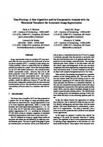
First, we have measured the cost ranges for each set of resource constraints, which are summarized in figure 16, normalized with respect to the ”no pruning” case. Note that cost ranges are reduced to at least 70% when pruning is enabled. At second, we counted the number of solutions which have hit the optimum latency and we evaluated the average percentage with respect to the total number of solutions. This percentage represents the average density of optimal solutions in the search space and it is presented in the shadowed rows of table 4, where ”nopru” and ”pru” stand for ”no pruning” and ”pruning”, respectively. Again, the results show that code– motion pruning increases the density of high–quality solutions in the search space. They also show that the tighter the resource constraints are, the more impact has code–motion pruning. This results can be interpreted as follows. When resources are scarce, such as in cases (a), (b), (e) and (f), only a small fraction of the potential parallelism can be accommodated within the available resources and, as a consequence, more code motions are pruned, since they would be inefficient. On the other hand, if resources are abundant, like in cases (c), (d), (g) and (h), most of the potential parallelism is accommodated by the available resources and there is no need to prune most code motions, as they contribute in the construction of high–quality solutions. Table 4 – The impact of code–motion pruning on the density of optima s2r [26] (a) (b) (c) (d) (e) (f) #alu 1 2 3 4 1 2 resources # mul 0 0 0 0 2 2 latency –– 14 8 8 8 12 8 nopru 1% 1% 41% 45% 1% 2% density pru 41% 16% 62% 62% 25% 16% nopru 26 17 0.9 0.9 24 17 CPU (s) pru 0.7 3.0 0.7 1.1 1.1 3.6 alu: 1–cycle ALU; mult: 2–cycle pipel. multiplier 1 single–port look–up table

(g) 3 2 8 31% 45% 17 1.1

(h) 4 2 8 34% 45% 1.4 1.1

Since in the synthesis of ASICs or in the code generation for ASIPs we want to use as few resources as possible, we are likely to observe, in practice, a huge unbalance between the potential parallelism and the exploitable parallelism, which is constrained by the available resources. This fact justifies the use of our code–motion pruning technique.

31

In order to compare the impact of the different densities of optima on search time, we also measured the average time to reach a given optimum. Here we have emulated a kind of random search for the optimal latencies shown in table 4. The average search times are reported under entry ”CPU”. Results show that code–motion pruning leads to a substantial improvement on search time under tight resource constraints.

9 CONCLUSIONS AND FUTURE WORK This paper shows how scheduling and code motion can be treated as a unified problem, while optimal solutions are kept in the search space. The problem was approached from the point of view of an optimization process where the construction of a solution is independent from the exploration of alternatives. It was shown how a permutation can be used to induce unrestricted code motions. Once the presence of optimal solutions in the search space was guaranteed by a better control over the construction procedure, we have shown that a pruning technique can ease the optimization process by exploiting constraints. Since control dependencies represent obstacles to exploit parallelism, we might be induced to violate them as often as possible. However, we conclude that control dependencies should also be exploited, in combination with resource constraints and data dependencies, in order to detect and prevent inefficient code motions. Our way to cast the problem and the experimental results allow us to conclude that such a code–motion pruning increases the density of high–quality solutions in the search space. Even though this paper focuses on a problem related to the early phases of a design flow, our constructive method can accommodate some extensions. As many alternative solutions are generated, it is possible to extend the constructor to keep track of other issues like register and interconnect usage, and the number of states. Those issues could then be captured in the cost function. This is convenient especially in the late phases of a design flow, where optimization has to take several design issues into account. As future work, we intend to cast loop pipelining into our constructive approach. Loops could be easily supported in our method with simple extensions, as they can be modeled with conditionals. Loops could then be ”broken” during scheduling and the back edges could be restored later into the state machine graph, like in [5] and [15]. However, such extensions would not allow exploitation of parallelism across different iteration of a loop. For this reason, we prefer to investigate loops as a further topic.

32

APPENDIX I. Proof for the pruning technique Theorem: Let Sm be a solution of the optimization problem described in section 2.2. Assume that Sm was constructed with algorithm 2 for a given P and let o be an operation assigned to BB j in Sm. Let d be ȱ delay(o) ȳ. If a solution Sn is obtained by moving o from BB j into BB i and it allocates exactly d extra cycle steps to accommodate the execution of o inside BB i, then cost(Sn) w cost(Sm). Proof: Let l(K), L(K) Ů 8 be the schedule lengths of a BB K before and after the motion, respectively. Let P, Q, R, S be BBs forming path pi : P ³Q ³R and path pj : P ³S ³R. Let ln and Ln be, respectively, the schedule lengths of path pn before and after motion. a) o was assigned to Q and allocates d steps inside P å L(P)=l(P)+ d a.1) No operation assigned to R can be moved into the allocated steps å L(R)=l(R),

L(S) w l(S)– d , L(Q) w l(Q)– d å Li w li and Lj w lj

a.2) There is an operation u assigned to R which can be moved into the allocated steps. As u depends or has resource conflicts with operations assigned to Q and S (topological permutation construction) å L(Q) w

l(Q)– d + ȱdelay(u)ȳ, L(S) w l(S)– d + ȱdelay(u)ȳ, L(R) w l(R)– ȱdelay(u)ȳ

å Li w li and Lj w lj b) o was assigned to R and allocates d steps inside both Q and S å L(Q)

= l(Q)+ d , L(S) = l(S)+ d , L(R) w l(R)– d å Li w li and Lj w lj

c) o was assigned to R and allocates d steps inside P å L(P) = l(P)+ d As o does not depend but has resource conflicts with operations assigned to Q and S (topological permutation construction) å L(Q)

= l(Q), L(S) = l(S), L(R) w l(R)– d å Li w li and Lj w lj

For a given P, solution Sn has path lengths greater than or equal to those in Sm. As any generalized code motions can be seen as ”compound” code motions built out of these basic code motions, and cost is monotonically increasing, we can conclude without loss of generality that cost(Sn) w cost(Sm). h

33

REFERENCES [1] S. Amellal and B. Kaminska, ”Functional Synthesis of Digital Systems with TASS,” IEEE Trans. on Computer Aided Design, 13(5): 537–552, May 1994. [2] R. Bergamaschi et al., ”Area and Performance Optimizations in Path Based Scheduling,” in Proc. European Conference on Design Automation, pp. 304–310, 1991. [3] R. Bergamaschi et al., ”Control–Flow Versus Data–Flow–Based Scheduling: Combining Both Approaches in an Adaptive Scheduling System,” in IEEE Trans. on VLSI Systems, 5(1), March 1997, pp. 82–100. [4] M. Berkelaar and L. van Ginneken, ‘‘Efficient Orthonormality Testing for Synthesis with Pass–Transistor Selectors,’’ in Proc. ACM/IEEE Int. Conference on Computer Aided Design, pp. 256–263, 1995. [5] R. Camposano, ”Path–based scheduling for synthesis,” IEEE Trans. on Computer Aided Design, 10(1): 85–93, Jan. 1991. [6] R. Camposano and J. Wilberg, ”Embedded System Design, ” Design Automation for Embedded Systems Journal, n. 1, pp. 5–50, 1996. [7] G. DeMicheli, Synthesis and Optimization of Digital Circuits, Mc Graw–Hill, 1994. [8] K. Ebcioglu and A. Nicolau, ”A global resource–constrained parallelization technique,” in Proc. of the ACM SIGARCH Int. Conference on Supercomputing, pp. 154–163, 1989. [9] J. Eijndhoven and L. Stok, ”A Data Flow Exchange Standard,” in Proc. European Conference on Design Automation, pp. 193–199, 1992. [10] J. A. Fisher, ”Trace Scheduling: A technique for global microcode compaction,” IEEE Trans. on Computers, vol. 30, July 1981. [11] R. Gupta and M.L. Soffa, ”Region Scheduling: An Approach for Detecting and Redistributing Parallelism,” in IEEE Trans. on Software Engineering, 16(4), Apr 1990, pp. 421–431. [12] M.Heijligers et al., ”NEAT: an Object Oriented High Level Synthesis Interface”, in Proc. IEEE Internation Symposium on Circuits and Systems, pp.1.233–1.236,1994. [13] M.Heijligers, The Application of Genetic Algorithms to High–Level Synthesis, PhD Thesis, Eindhoven University of Technology, The Netherlands, 1996. [14] J. Henkel and R. Ernst. ”A Path–based Technique for Estimating Hardware Runtime in HW/SW–cosynthesis”, in Proc. ACM/IEEE Int. Symposium on System Synthesis, pp.116–121, 1995. [15] S.Huang et al., ”A tree–based scheduling algorithm for control dominated circuits,” in Proc. ACM/IEEE Design Automation Conference, pp–578–58, 1993. [16] A.Kifli et al.,”A Unified Scheduling Model for High–Level Synthesis and Code Generation,” in Proc. European Design and Test Conference, pp.234–238, 1995. [17] A. Kifli, Global Scheduling in High–Level Synthesis and Code Generation for Embedded Processors. PhD Thesis, Department of Electrical Engineering, K. U. Leuven, Belgium, 1996. [18] T. Kim et al., ”A Scheduling Algorithm for Conditional Resource Sharing – A Hierarchical Reduction Approach”, IEEE Trans. on Computer Aided Design, 13(4):425–438, Apr 1994. [19] M. S. Lam and R. P. Wilson, ”Limits of Control Flow on Parallelism,” ACM/IEEE Int. Symposium on Computer Architecture., 1992, pp. 46–57. [20] R.Leupers and P.Marwedel, ”Time constrained Code Compaction for DSPs”, in Proc. ACM/IEEE Int. Symposium on System Synthesis, pp.54–59, 1995. [21] S.–M. Moon and K. Ebcioglu, ”An Efficient Resource–Constrained Global Scheduling Technique for Superscalar and VLIW processors,” in Proc. Int. Symposium and Workshop on Microarchitecture (MICRO–25), Dec. 1992, pp. 55–71. [22] T. Nakatani and K. Ebcioglu, ”Making Compaction–Based Parallelization Affordable,” in IEEE Trans. on Parallel and Distributed Systems, 4(9), Sept. 1993, 1014–1029. [23] A. Nicolau, ”Uniform Parallelism Exploitation in Ordinary Programs”, in Proc. Int. Conference on Parallel Processing, pp. 614–618, 1985.

34

[24] C. Papadimitriou and K. Steiglitz, Combinatorial optimization: algorithms and complexity, Prentice Hall, 1982. [25] R. Potasman et al., ‘‘Percolation Based Synthesis,’’ in Proc. ACM/IEEE Design Automation Conference, pp. 444–449, 1990. [26] I.Radivojevic and F.Brewer, ”A New Symbolic Technique for Control Dependent Scheduling,” IEEE Trans. Computer Aided Design ,15(1):45–57, 1996. [27] M. Rim and R. Jain, ”Representing conditional branches for high–level synthesis applications,” in Proc. ACM/IEEE Design Automation Conference, pp.106–111, 1992. [28] M. Rim, et al., ”Global Scheduling with Code–Motions for High–Level Synthesis Applications,” IEEE Trans. on VLSI Systems, vol. 3, no. 3, Sept. 1995, pp. 379–392. [29] L.C.V. dos Santos et al.,‘‘A Constructive Method for Exploiting Code Motion,’’ in Proc. ACM/IEEE Int. Symposium on System Synthesis, pp. 51–56, 1996. [30] M. Smith, M. Horowitz, and M. Lam., ”Efficient Superscalar Performance Through Boosting,” in Proc. International Conference on Architectural Support for Programming Languages and Operating Systems (ASPLOS–5), pp. 248–259, 1992. [31] K. Wakabayashi and T. Yoshimura, ”A resource sharing and control synthesis method for conditional branches,” in Proc. ACM/IEEE Int. Conference on Computer Aided Design, pp.62–65, 1989. [32] K. Wakabayashi and H. Tanaka, ”Global scheduling independent of control dependencies based on condition vectors,” in Proc. ACM/IEEE Design Automation Conference, pp.112–115, 1992.

35