Feb 5, 2013 - f : N â N. The judgment is valid if cpP is defined on all inputs, and ... If there exists a closed complexity proof ⢠P : f, then the judgement ⢠P : f is.
A Combination Framework for Complexity∗ 1
Martin Avanzini1, and Georg Moser1 Institute of Computer Science, University of Innsbruck, Austria {martin.avanzini,georg.moser}@uibk.ac.at
arXiv:1302.0973v1 [cs.CC] 5 Feb 2013
February 6, 2013
In this paper we present a combination framework for polynomial complexity analysis of term rewrite systems. The framework covers both derivational and runtime complexity analysis. We present generalisations of powerful complexity techniques, notably a generalisation of complexity pairs and (weak) dependency pairs. Finally, we also present a novel technique, called dependency graph decomposition, that in the dependency pair setting greatly increases modularity. We employ the framework in the automated complexity tool TCT. TCT implements a majority of the techniques found in the literature, witnessing that our framework is general enough to capture a very brought setting.
1 Introduction In order to measure the complexity of a term rewrite system (TRS for short) it is natural to look at the maximal length of derivation sequences—the derivation length—as suggested by Hofbauer and Lautemann in [13]. The resulting notion of complexity is called derivational complexity. Hirokawa and the second author introduced in [10] a variation, called runtime complexity, that only takes basic or constructor-based terms as start terms into account. The restriction to basic terms allows one to accurately express the complexity of a program through the runtime complexity of a TRS. Noteworthy both notions constitute an invariant cost model for rewrite systems [5, 4]. The body of research in the field of complexity analysis of rewrite systems provides a wide range of different techniques to analyse the derivational and runtime complexity of rewrite systems, fully automatically. Techniques range from direct methods, like polynomial path orders [6, 3] and other suitable restrictions of termination orders [8, 18], to transformation techniques, maybe most prominently adaptions of the dependency pair method [10, 11, 12, 19], semantic labeling over finite carriers [2], methods to combine base techniques [22] and the weight gap principle [10, 22]. Se also [17] for the state-of-the-art in complexity analysis of term rewrite systems. In particular the dependency pair method for complexity analysis allows for a wealth of techniques originally intended for termination analysis, foremost (safe) ∗
This work was partially supported by FWF (Austrian Science Fund) project I-603-N18.
1
reduction pairs [10, 12], various rule transformations [19], and usable rules [10, 12] are used in complexity analysers. Some very effective methods have been introduced specifically for complexity analysis in the context of dependency pairs. For instance, path analysis [10, 12] decomposes the analysed rewrite relation into simpler ones, by treating paths through the dependency graph independently. Knowledge propagation [19] is another complexity technique relying on dependency graph analysis, which allows one to propagate bounds for specific rules along the dependency graph. Besides these, various minor simplifications are implemented in tools, mostly relying on dependency graph analysis. With this paper, we provide foremost following contributions. 1. We propose a uniform combination framework for complexity analysis, that is capable of expressing the majority of the rewriting based complexity techniques in a unified way. Such a framework is essential for the development of a modern complexity analyser for term rewrite systems. The implementation of our complexity analyser TCT, the Tyrolean Complexity Tool, closely follows the here proposed formalisation. Noteworthy, TCT is the only tool that is ably to participate in all four complexity sub-divisions of the annual termination competition.1 2. A majority of the cited techniques were introduced in a restricted respectively incompatible contexts. For instance, in [22] derivational complexity of relative TRSs are considered. Conversely, [10, 12] nor [19] treat relative systems, and restrict their attention to basic, aka constructor-based, start terms. Where non-obvious, we generalise these techniques to our setting. Noteworthy, our notion of P-monotone complexity pair generalises complexity pairs from [22] for derivational complexity, µ-monotone complexity pairs for runtime complexity analysis recently introduced in [12], and safe reduction pairs introduced in [10] that work on dependency pairs.2 We also generalise the two different forms of dependency pairs for complexity analysis introduced in [10] and respectively for innermost rewriting in [19]. This for instance allows our tool TCT to employ these very powerful techniques on a TRS R relative to some theory expressed as a TRS S. 3. Besides some simplification techniques, we introduce a novel proof technique for runtime-complexity analysis, called dependency graph decomposition. Inspired by cycle analysis [21], this technique in principle allows the analysis of two disjoint portions of the dependency graph (almost) independently. Resulting sub-problems are syntactically of simpler form, and so the analysis of this sub-problems is often significantly easier. Importantly, the sub-problems are usually also computational simpler in the sense that their complexity is strictly smaller than the one of the input problem. More precisely, if the complexity of the two generated sub-problems is bounded by a function in O(f ) respectively O(g), then the complexity of the input is bounded by O(f ·g), and often this bound is tight. This paper is structured as follows. In the next section we cover some basics. Our combination framework is then introduced in Section 3. In Section 4 we introduce µ-monotone orders. In Section 5 we introduce dependency pairs for complexity analysis, and reprove 1 2
C.f. http://termcomp.uibk.ac.at/. In [19] safe reductions pairs are called com-monotone reduction pairs.
2
soundness of weak dependency pairs and dependency tuples. In Section 6 we introduce aforementioned simplification and dependency graph decomposition, and finally in Section 7 we conclude.
2 Preliminaries Let R be a binary relation. The transitive closure of R is denoted by R+ and its transitive and reflexive closure by R∗ . For n ∈ N we denote by Rn the n-fold composition of R. The binary relation R is well-founded if there exists no infinite chain a0 , a1 , . . . with ai R ai+1 for all i ∈ N. Moreover, we say that R is well-founded on a set A if there exists no such infinite chain with a0 ∈ A. The relation R is finitely branching if for all elements a, the set {b | a R b} is finite. A preorder is a reflexive and transitive binary relation. A (directed) hypergraph with labels in L is a triple G = (N, E, lab) where N is a set of nodes, E ⊆ N × P(N ) a set of edges, and lab : N ∪ E → L a labeling function. For an edge e = hu, {v1 , . . . , vn }i ∈ E the node u is called the source, and the nodes v1 , . . . , vn are called the targets of e. We keep the convenient that every node is the source of at most one edge. If lab(u) = l for node u ∈ N then u is called an l-node, this is extended to labels K ⊆ L in the obvious way. Correspondingly an edge e ∈ E is called a l-edge (respectively K-edge) if lab(e) = l (lab(e) ⊆ K). We denote by − ⇀G the successor relation in G, that is, u − ⇀G v if there exists an edge e = hu, {v1 , . . . , vn }i ∈ E with v ∈ {v1 , . . . , vn }. For a label l ∈ L we set l K u− ⇀ ⇀ ⇀∗G v holds then v G v (respectively u − T v) if the edge e is an l-edge (K-edge). If u − is called reachable from u (in G). If every node v ∈ N is reachable from a designated node u, the root of G, then G is called a hypertree, or simply tree. We assume familiarity with rewriting [7] and just fix notations. We denote by V a countably infinite set of variables and by F a signature. The signature F and variables V are fixed throughout the paper, the set of terms over F and V is written as T (F, V). Throughout the following, we suppose a partitioning of F into constructors C and defined symbols D. The set of basic terms f (s1 , . . . , sn ), where f ∈ D and arguments si (i = 1, . . . , n) contain only variables or constructors, is denoted by Tb . Terms are denoted by s, t, . . . , possibly followed by subscripts. We use s|p to refer to the subterm of s at position p. We denote by |t| the size of t, i.e., the number of symbols occurring in t. A rewrite relation → is a binary relation on terms closed under contexts and stable under substitutions. We use R, S, Q, W to refer to term rewrite systems (TRSs for short), i.e., sets of rewrite rules that obey the usual restrictions. We denote by NF(R) the normal forms of R, and abusing notation we extend this notion to binary relations → on terms in the obvious way: NF(→) is the least set of terms t such that t → s does not hold for any term t. For a set of terms T ⊆ T (F, V), we denote by →(T ) the least set containing T and that is closed under →: s ∈ →(T ) and s → t implies t ∈ →(T ). Q For two TRSs Q and R, we define s − →R t if there exists a context C, substitution σ, and rule f (l1 , . . . , ln ) → r such that s = C[f (l1 σ, . . . , ln σ)], t = C[rσ] and all arguments li σ (i = 1, . . . , n) are Q normal forms. If Q = ∅, we sometimes drop Q and write − →R instead ∅ of − → . Note that → − is smallest rewrite relation containing R and thus corresponds to R R the usual definition of rewrite relation of R. The innermost rewrite relation of a TRS R is R Q Q R ∗ R R ∗ given by − →R R. We extend − →R to a relative setting and define − →R/S := − →S · − →R · − →S . The derivation height of a term t with respect to a binary relation → on terms is given
3
by dh(t, →) max{n | ∃t1 , . . . , tn . t → t1 → · · · → tn }. Note that the derivation height dh is a partial function, but it is defined on all inputs when → is well-founded and finitely branching. We will not presuppose that → satisfies these properties, but our techniques Q will always imply that dh(t, →) is well-defined. We emphasise that dh(t, − → R/S ), if defined, Q binds the number of R steps in all − →R∪S derivations starting from t. Let T be a set of terms, and define cp(n, T, →) := max{dh(t, →) | ∃t ∈ T, |t| 6 n}. The derivational complexity of a TRS R is given by dcR (n) := cp(n, T (F, V), − →R ) for all n ∈ N, the runtime complexity takes only basic terms as starting terms T into account: rcR (n) := cp(n, Tb♯ , − →R ) for all R n ∈ N. By exchanging − →R with − →R we obtain the notions of innermost derivational or runtime complexity respectively.
3 The Combination Framework At the heart of our framework lies the notion of complexity processor, or simply processor. A complexity processor dictates how to transform the analysed input problem into subproblems (if any), and how to relate the complexity of the obtained sub-problems to the complexity of the input problem. In our framework, such a processor is modeled as a set of inference rule ⊢ P1 : f1 · · · ⊢ Pn : fn ⊢ P: f , over judgements of the form ⊢ P : f . Here P denotes a complexity problem (problem for short) and f : N → N a bounding function. The validity of a judgement ⊢ P : f is given when the function f binds the complexity of the problem P asymptotically. The next definition introduces complexity problems formally. Conceptually a complexity Q problem P constitutes of a rewrite relation − →R/S represented by the finite TRSs R, S and Q, and a set of starting terms T . Definition 1 (Complexity Problem, Complexity Function). 1. A complexity problem P ( problem for short) is a quadruple hS, W, Q, T i, in notation hS/W, Q, T i, where S, W, Q are TRSs and T ⊆ T (F, V) a set of terms. 2. The complexity (function) cpP : N → N of P is defined as the partial function Q cpP (n) := max{dh(t, − → S/W ) | t ∈ T and |t| 6 n} .
Below P, possibly followed by subscripts, always denotes a complexity problem. Consider a problem P = hS/W, Q, T i. We call S and W the strict and respectively weak rules, or component of P. The set T is called the set of starting terms of P. We sometimes write Q l → r ∈ P for l → r ∈ S ∪ W. We denote by − →P the rewrite relation − → S∪W . A derivation t− →P t1 → − P · · · is also called a P-derivation (starting from t). Observe that the derivational complexity of a TRS R corresponds to the complexity function of hR/∅, ∅, T (F, V)i. By exchanging the set of starting terms to basic terms we can express the runtime complexity of a TRS R. If the starting terms are all basic terms, we call such a problem also a runtime complexity problem. Likewise, we can treat innermost rewriting by using Q = R. For the case NF(Q) ⊆ NF(S ∪ W), that is when − →P is included in the innermost rewrite relation of R ∪ S, we also call P an innermost complexity problem.
4
Example 2. Consider the rewrite system R× given by the four rules a: 0 + y → y
b : s(x) + y → x + y
c: 0 × y → 0
d : s(x) × y → y + (x × y) ,
and let Tb denote basic terms with defined symbols +, × and constructors s, 0. Then P× := hR× /∅, R× , Tb i is an innermost runtime complexity problem, in particular the complexity of P equals the innermost runtime complexity of R× . Q Note that even if − → S/W is terminating, the complexity function is not necessarily defined on all inputs. For a counter example, consider the problem P1 := hS1 /W1 , ∅, {f(⊥)}i where S1 := {g(s(x)) → g(x)} and W1 := {f(x) → f(s(x)), f(x) → g(x)}. Then the set of − →S1 /W1 reductions of f(⊥) is given by the family
f(⊥) − →S1 /W1 g(sn (⊥)) − →nS1 /W1 g(⊥) , for n ∈ N. So − →S1 /W1 is well-founded, but dh(f(⊥), − →S1 /W1 ) = cpP1 (m) (m > 2) is unQ defined. If − → is well-founded and finitely branching then cpP is defined on all inputs, S/W by K¨ onigs Lemma. This condition is sufficient but not necessary. The complexity function of the problem P2 := hS2 /W1 , ∅, {f(⊥)}i, where S2 := {g(x) → x}, is constant but f(⊥) − →S2 /W1 sn (⊥) for all n ∈ N, i.e, − →S2 /W1 is not finitely branching. In this work we do not presuppose that the complexity function is defined on all inputs, instead, this will be determined by our methods. To compare partial functions in proofs, we use Kleene equality: two partial functions f, g : N → N are equal, in notation f ≃ g, if for all n ∈ N either f (n) and g(n) are defined and f (n) = g(n), or both f (n) and g(n) are undefined. We abuse notation and write f & g if for all n ∈ N with f (n) defined, f (n) & g(n) with g(n) defined holds. Then f ≃ g if and only if f & g and g & f . Definition 3 (Judgement, Processor, Proof). 1. A (complexity) judgment is a statement ⊢ P : f where P is a complexity problem and f : N → N. The judgment is valid if cpP is defined on all inputs, and cpP ∈ O(f ). 2. A complexity processor Proc ( processor for short) is an inference rule ⊢ P1 : f1
· · · ⊢ Pn : fn Proc ⊢ P: f ,
over complexity judgements. The problems P1 , . . . , Pn are called the sub-problems generated by Proc on P. The processor Proc is sound if cpP1 ∈ O(f1 ) ∧ · · · ∧ cpPn ∈ O(fn )
=⇒
cpP ∈ O(f ) ,
it is complete if the inverse direction holds. 3. Let empty denotes the axiom ⊢ h∅/W, Q, T i : f for all TRSs W and Q, set of terms T and f : N → N. A complexity proof ( proof for short) of a judgement ⊢ P : f is a deduction from the axiom empty and assumptions ⊢ P1 : f1 , . . . , ⊢ Pn : fn using sound processors, in notation P1 : f1 , . . . , Pn : fn ⊢ P : f .
5
We say that a complexity proof is closed if its set of assumptions is empty, otherwise it is open. We follow the usual convention and annotate side conditions as premises to inference rules. Soundness of a processor guarantees that validity of judgements is preserved. Completeness ensures that a deduction can give asymptotically tight bounds. The next lemma verifies that our formal system is correct. Lemma 4. If there exists a closed complexity proof ⊢ P : f , then the judgement ⊢ P : f is valid. Proof. The lemma follows by a standard induction on the length of proofs, exploiting that the underlying set of processors is sound.
4 Orders for Complexity Maybe the most obvious tools for complexity analysis in rewriting are reduction orders, in particular interpretations. Consequently these have been used quite early for complexity analysis. For instance, in [8] polynomial interpretations are used in a direct setting in order to estimate the runtime complexity analysis of a TRS. In [22] so called complexity pairs are employed to estimate the derivational complexity in a relative setting. Weakening monotonicity requirements of complexity pairs gives rise to a notion of reduction pair, so called safe reduction pairs [10], that can be used to estimate the runtime complexity of dependency pair problems, cf. also [12, 19]. In the following, we introduce P-monotone complexity pairs, that give a unified account of the orders given in [8, 22, 12, 19]. We fix a complexity problem P = hS/W, Q, T i. Consider a proper order ≻ on terms, and let G denote a mapping associating a term with a natural number. Then ≻ is G-collapsible Q (on P) if G(s) > G(t) whenever s − →S/W t and s ≻ t holds for all terms s ∈ − →P (T ) reachable from T . If in addition G(t) is asymptotically bounded by a function f : N → N in the size of t for all start terms t ∈ T , i.e., G(t) ∈ O(f (|t|)) for t ∈ T , we say that ≻ induces the complexity f on P. We note that only in pathological cases an order is not collapsible on P. In particular polynomial and matrix interpretations [7, 14] are collapsible, and also recursive path order [7] are. All these termination techniques have also been suitable tamed so that the induced complexity can be given by a polynomial [8, 16, 3], for runtime and partly also for derivational complexity. Consider an order ≻ that induces the complexity f on P. If this order includes the relation Q − →S/W , the judgement ⊢ P : f is valid. To check the inclusion, we consider complexity pair (%, ≻), where % denotes a preorder % compatible with ≻, in the sense that % · ≻ · % ⊆ ≻ holds. It is obvious that when both orders are monotone and stable under substitutions, Q the assertions W ⊆ % and S ⊆ ≻ imply − → S/W ⊆ ≻ as desired. Monotonicity ensures that the orders are closed under contexts. Of course, closure under context is only required on argument positions that can be rewritten in reductions of staring terms T . Such argument positions are called usable below. In [12] it is shown how to precisely capture reductions from basic terms by context sensitive rewriting [15], and conclusively µ-monotone orders [23], can be exploited for runtime complexity analysis. The parameter µ denote a replacement map, i.e., a map that assigns to every n-ary function symbol f ∈ F a subset of its argument positions: µ(f ) ⊆ {1, . . . , n}. In the realm of context sensitive rewriting, the replacement map governs under which argument
6
positions a rewrite step is allowed. Here we use µ to designate which argument positions are usable. Denote by Posµ (t) the µ-replacing positions in t, defined as Posµ (t) := {ǫ} if t is a variable, and Posµ (t) := {ǫ} ∪ {i·p | i ∈ µ(f ) and p ∈ Posµ (ti )} for t = f (t1 , . . . , tn ). For a binary relation → on terms we denote by Tµ (→) the least set of terms s such that whenever s|p 6∈ NF(→), then p is a µ-replacing position. The following constitutes an adaption of usable replacement maps [12] to our setting. Definition 5. Let P be a complexity problem with starting terms T and let R denote a set of rewrite rules. A replacement map µ is called a usable replacement map for R in P, if Q →P (T ) ⊆ Tµ (− − → R ). Hence a usable replacement map µ of R in P determines under which argument positions an R step is possible. This is illustrated by the following example. Example 6 (Example 2 continued). Consider the derivation →P× s(s(0)) + (0 × s(s(0))) − →P× s(s(0)) + 0 − →P× s(s(0) + 0) − →P× · · · , s(0) × s(s(0)) − where redexes are underlined. Observe that e.g. multiplication occurs only under the second argument position of addition in this sequence. The replacement map µ× , defined by µ× (+) = {2} and µ× (×) = µ× (s) = ∅, thus constitutes a usable replacement map for the multiplication rules {c, d} in P× . Since the argument position of s is not usable in µ× , the last step witnesses that µ× does not designate a usable replacement map for the addition rules {a, b}. We say that an order ≻ is µ-monotone if it is monotone on µ positions, in the sense that for all function symbols f , if i ∈ µ(f ) and si ≻ ti then f (s1 , . . . , si , . . . , sn ) ≻ f (s1 , . . . , ti , . . . , sn ) holds. Consider a usable replacement map µ for a TRS R in P, and let ≻ be a µ-monotone order stable under substitution. Compatibility of ≻ with R ensures that every R step in a P derivation of t ∈ T is oriented by ≻: Lemma 7. Let µ be a usable replacement map for R in P, and let ≻ denote a µ-monotone order that is stable under substitutions. If R ⊆ ≻ holds, i.e., rewrite rules in R are oriented Q from left to right, then s − → →P (T ). R t implies s ≻ t for all terms s ∈ − Proof. Since µ is a usable replacement map for R in P, it suffices to show the claim for Q Q s ∈ Tµ (− → →R,p t, hence p ∈ Posµ (t). We show that for every prefix q of p, R ). Suppose s − s|q ≻ t|q holds. Consider a prefix q of p. The proof is by induction on |p| − |q|. The base case q = p is covered by compatibility and stability under substitutions. For the inductive step, consider prefix q·i of p, where by induction hypothesis s|q·i ≻ t|q·i . Since p ∈ Posµ (s) and q·i is a prefix of p it is not difficult to see that i ∈ µ(f ). Thus s|q = f (s1 , . . . , s|q·i , . . . , sn ) ≻ f (s1 , . . . , t|q·i , . . . , sn ) = s|q , follows by µ-monotonicity of ≻. From the claim, the lemma is obtained using q = ǫ. The next definition of P-monotone complexity pair (%, ≻) ensures that % and ≻ are sufficiently monotone, in the sense that the inclusions W ⊆ % on weak and S ⊆ ≻ on strict Q Q rules of P extend to − →W respectively − →S , according Lemma 7.
7
Definition 8 (Complexity Pair, P-monotone). 1. A complexity pair is a pair (%, ≻), such that % is a stable preorder and ≻ a stable order with % · ≻ · % ⊆ ≻. 2. Suppose % is µW -monotone for a usable replacement map of W in P, and likewise ≻ is µS -monotone for a usable replacement map of S in P. Then (%, ≻) is called P-monotone. When the set of starting terms is unrestricted, as for derivational complexity analysis, then trivially only the full replacement map is usable for rules of P. In this case, our notion of complexity pair collapses to the one given by Zankl and Korp [22]. We emphasise that in contrast to [12], our notion of complexity pair is parameterised in separate replacements for % and ≻. By this separation we can recast (safe) reduction pairs originally proposed in [10], employed in the dependency pair setting below, as instances of complexity pairs (cf. Lemma 21). It is undecidable to determine if µ is a usable replacement map for rules R in P. Exploiting that for runtime-complexity the set of starting terms consists of basic terms only, Hirokawa and Moser [12] define an algorithm that computes good approximations of usable replacement maps µ, both for the case of full and innermost rewriting. The next lemma verifies that complexity pairs bind the length of derivations. Lemma 9. Consider a P-monotone complexity pair (%, ≻) that is G-collapsible on P, and Q compatible in the sense that W ⊆ % and S ⊆ ≻. Then dh(t, − → S/W ) is defined for all t ∈ T , Q in particular dh(t, − →S/W ) 6 G(t). Q Q Q Proof. Consider an arbitrary derivation t = t0 − →S/W t1 − → → S/W t2 − S/W · · · for some Q →S/W ti+1 for some i ∈ N. Using compatibility term t ∈ T . Consider a sub-sequence ti − and P-monotonicity we see ti %∗ · ≻ · %∗ ti+1 by Lemma 7, using that % is a preorder we even have ti % · ≻ · % ti+1 and hence ti ≻ ti+1 by definition of complexity pair. Since ≻ is Q G-collapsible on − → S/W we conclude G(t) = G(t0 ) > G(t1 ) > G(t2 ) > · · · . Conclusively the sequence t0 , t1 , t2 , . . . is finite, and its length is bounded by G(t). The lemma follows.
As an immediate consequence we obtain our first processor. Theorem 10 (Complexity Pair Processor). Let (%, ≻) be a P-monotone complexity pair such that ≻ induces the complexity f on P. The following processor is sound: S⊆≻ W ⊆% CP ⊢ hS/W, Q, T i : f . A variation of the complexity pair processor, that iterative orients disjoint subsets of S, occurred first in [22]. The following processor constitutes a straight forward generalisation of [22, Theorem 4.4] to our setting. Theorem 11 (Decompose Processor [22]). The following processor is sound: ⊢ hS1 /S2 ∪ W, Q, T i : f ⊢ hS2 /S1 ∪ W, Q, T i : g decompose ⊢ hS1 ∪ S2 /W, Q, T i : f + g .
8
Proof Outline. Obviously the number of S1 ∪ S2 steps in a derivation is given by the sum of S1 and respectively S2 steps in this derivation. The effect of applying the complexity pair processor on one of the resulting sub-problems, for instance hS1 /S2 ∪ W, Q, T i, is to move the strictly oriented rules S1 to the weak component. This is demonstrated in the following proof, that was automatically found by our complexity prover TCT. The following proof was found by our tool TCT demonstrates this. Example 12 (Examples 2 and 6 continued). Consider the linear polynomial interpretation A over N such that 0A = 0, sA (x) = x, x +A y = y and x ×A y = 1. Let Pc := h{c}/{a, b, d}, R× , Tb i denote the problem that accounts for the rules c : 0 × y → y in P× . The induced order >A together with its reflexive closure >A forms a Pc -monotone complexity pair (>A , >A ) that induces linear complexity on Pc . Here monotonicity can be shown using the replacement maps given in Example 6. The following depicts a complexity proof h{a, b, d}/{c}, R× , Tb i : g ⊢ P× : λn.n + g. {c} ⊆ >A {a, b, d} ⊆ >A CP ⊢ h{c}/{a, b, d}, R× , Tb i : λn.n ⊢ h{a, b, d}/{c}, R× , Tb i : g decompose ⊢ P× : λn.n + g . The above complexity proof can now be completed iterative, on the simpler problem h{a, b, d}/{c}, R× , Tb i. Since the complexity of P× is bounded below by a quadratic polynomial, one however has to use a technique beyond linear polynomial interpretations. We remark that the decompose processor finds applications beyond its combination with complexity pairs, our tool TCT uses this processor for instance for the separation of independent components in the dependency graph.
5 Dependency Pairs for Complexity Analysis The introduction of the dependency pair (DP for short) [1], and its prominent reincarnation in the dependency pair framework [21], drastically increased power and modularity in termination provers. It is well established that the DP method is unsuitable for complexity analysis. The induced complexity is simply too high [20], in the sense that the complexity of R is not suitably reflected in its canonical DP problem. Hirokawa and Moser [10] recover this deficiency with the introduction of weak dependency pairs. Crucially, weak dependency pairs group different function calls in right-hand sides, using compound symbols. In this section, we first introduce a notion of dependency pair complexity problem (DP problem for short), a specific instance of complexity problem. In Theorem 20 and Theorem 24 we then introduce the weak dependency pair and dependency tuples processors, that construct from a runtime-complexity problem its canonical DP problem. We emphasise that both processors are conceptually not new, weak dependency pairs were introduced in [10], and the seminal paper of Noschinski et al. [19] introduced dependency tuples. In this work we provide alternative proofs of central theorems from [10] and [19]. Unlike in the cited literature, we show a direct simulation that also accounts for weak rules, conclusively our processors provide a generalisation of [10, 19]. Consider a signature F that is partitioned into defined symbols D and constructors C. Let t ∈ T (F, V) be a term. For t = f (t1 , . . . , tn ) and f ∈ D, we set t♯ = f ♯ (t1 , . . . , tn )
9
where f ♯ is a new n-ary function symbol called dependency pair symbol. For t not of this shape, we set t♯ = t. The least extension of the signature F containing all such dependency pair symbols is denoted by F ♯ . For a set T ⊆ T (F, V), we denote by T ♯ the set of marked terms T ♯ = {t♯ | t ∈ T }. Let Ccom = {c0 , c1 , . . . } be a countable infinite set of fresh compound symbols, where we suppose ar(cn ) = n. Compound symbols are used to group calls in dependency pairs for complexity (dependency pairs or DPs for short). We define com(t) = t, and otherwise com(t1 , . . . , tn ) = cn (t1 , . . . , tn ) where cn ∈ Ccom . Definition 13 (Dependency Pair, Dependency Pair Complexity Problem). 1. A dependency pair ( DP for short) is a rewrite rule l♯ → com(r1♯ , . . . , rn♯ ) where l, r1 , . . . , rn ∈ T (F, V) and l is not a variable. 2. Let S and W be two TRSs, and let S ♯ and W ♯ be two sets of dependency pairs. A complexity problem hS ♯ ∪ S/W ♯ ∪ W, Q, T ♯ i with T ♯ ⊆ Tb♯ is called a dependency pair complexity problem (or simply DP problem). We keep the convention that R, S, W, . . . are TRSs over T (F, V), whereas R♯ , S ♯ , W ♯ , . . . always denote sets of dependency pairs. Example 14 (Example 2 continued). Denote by S×♯ the dependency pairs 1 : s(x) +♯ y → x +♯ y
2 : 0 +♯ y → c0
3 : s(x) ×♯ y → c2 (y +♯ (x × y), x ×♯ y)
4 : 0 ×♯ y → c0 ,
and let Tb♯ be the (marked) basic terms with defined symbols +♯ , ×♯ and constructors s, 0. Then P×♯ := hS×♯ /R× , R× , Tb♯ i, where R× are the rules for addition and multiplication depicted in Example 2, is a DP problem. We anticipate that the DP problem P×♯ reflects the complexity of our multiplication problem P× , compare Theorem 24 below. For the remaining of this section, we fix a DP problem P ♯ = hS ♯ ∪ S/W ♯ ∪ W, Q, T ♯ i. Call an n-holed context C a compound context if it contains only compound symbols. Consider the P×♯ derivation →P ♯ c2 (s(0) +♯ ( s(0) × s(0) ), s(0) ×♯ s(0)) s(s(0)) ×♯ s(0) − ×
→∗P ♯ − ×
c2 (s(0) +♯ s(0), s(0) ×♯ s(0))
− 2P ♯ c2 (0 +♯ s(0), c2 (s(0) +♯ 0, 0 ×♯ s(0))) . → ×
Observe that any term in the above sequence can be written as C[t1 , . . . , tn ] where C is a maximal compound context, and t1 , . . . , tn are marked terms without compound symbols. For instance, the last term in this sequence is given as C1 [0 +♯ s(0), s(0) +♯ 0, 0 ×♯ s(0)] for C1 := c2 (✷, c2 (✷, ✷)). This holds even in general, but with the exception that t1 , . . . , tn are not necessarily marked. Note that such an unmarked term ti (i ∈ {1, . . . , n}) can only result from the application of a collapsing rules l♯ → x for x a variable, which is permitted by our ♯ , defined as formulation of dependency pair. We capture this observation with the set T→ ♯ the least extension of T (F, V) and T (F, V) that is closed under compound contexts. Then the following observation holds.
10
s(s(0)) ×♯ s(0) s(x) ×♯ y → c2 (y +♯ (x × y), x ×♯ y)
s(0) +♯ (s(0) × s(0))
s(0) ×♯ s(0)
s(x) × y → y + (x × y) s(x) ×♯ y → c2 (y +♯ (x × y), x ×♯ y)
s(0) +♯ s(0)
s(0) +♯ 0
0 ×♯ s(0)
s(x) +♯ y → x +♯ y
0 +♯ s(0)
Figure 1: P×♯ Derivation Tree of s(s(0)) ×♯ s(0). ♯ ) ⊆ T ♯ . In particular, Lemma 15. For every TRS R and DPs R♯ , we have − →R♯ ∪R (T→ → ♯ ♯ →P ♯ (T ) ⊆ T→ follows. − ♯ where C is a maximal compound context. Suppose Proof. Let s = C[s1 , . . . , sn ] ∈ T→ s− →R♯ ∪R t. Since C contains only compound symbols, it follows that t = C[s1 , . . . , ti , . . . , sn ] ♯ . Conclusively t ∈ T ♯ and where si → − R♯ ∪R ti for some i ∈ {1, . . . , n}, where again ti ∈ T→ → the first half of the lemma follows by inductive reasoning. From this the second half of the ♯ and taking R♯ := S ♯ ∪ W ♯ and R := S ∪ W. lemma follows, using that T ♯ ⊆ T→ ♯ for a maximal compound context C. Any reConsider a term t = C[t1 , . . . , tn ] ∈ T→ duction of t consists of independent sub-derivations of ti (i = 1, . . . , n), which are possibly interleaved. To avoid reasoning up to permutations of rewrite steps, we introduce a notion of derivation tree that disregards the order of parallel steps under compound contexts.
Definition 16. Let t ∈ T ♯ (F, V) ∪ T (F, V). The set of P ♯ derivation trees of t, in notation DTreeP ♯ (t), is defined as the least set of labeled trees such that: 1. T ∈ DTreeP ♯ (t) where T consists of a unique node labeled by t. Q 2. Suppose t − →{l→r} com(t1 , . . . , tn ) for l → r ∈ P ♯ and let Ti ∈ DTreeP ♯ (ti ) for i = 1, . . . , n. Then T ∈ DTreeP ♯ (t), where T is a tree with children Ti (i = 1, . . . , n), the root of T is labeled by t, and the edge from the root of T to its children is labeled by l → r.
Consider a P ♯ derivation tree T . Note that an edge e = hu, {v1 , . . . , vn }i in T precisely corresponds to a P ♯ step, in the sense that if u is labeled by a term t and vi (i = 1, . . . , n) Q ♯ by ti , then u − → l→r com(t1 , . . . , tn ) holds, with l → r ∈ P the label of e. In this case, we also say that the rule l → r was applied at node u in T . It is not difficult to see that from T one can always extract a P ♯ derivation D, by successively applying the rewrite rules in T , starting from the root. In this case we also say that D corresponds to T , and vice versa. For instance, the derivation tree given in Figure 1 and the derivation given below Example 14 are corresponding. Inversely, we can also associate to every P ♯ derivation D starting from t ∈ T (F, V) ∪ T ♯ (F, V) a P ♯ derivation tree T corresponding to D, so that there is a one-to-one correspondence between applied rules in T and rules applied in D. This leads to following characterisation of the complexity function of P ♯ . Here |T |R♯ ∪R refers to the number of applications of a rule l → r ∈ R♯ ∪ R in T , more precisely, |T |R♯ ∪R is the number of edges in T labeled by a rule l → r ∈ R♯ ∪ R.
11
Lemma 17. For every t ∈ T (F, V) ∪ T ♯ (F, V), we have Q dh(t, − →S ♯ ∪S/W ♯ ∪W ) ≃ max{|T |S ♯ ∪S | T is a P ♯ -derivation tree of t} .
In particular cpP ♯ (n) ≃ max{|T |S ♯ ∪S | T is a P ♯ -derivation tree of t ∈ T with |t| 6 n} holds. Proof. For a term t, abbreviate max{|T |S ♯ ∪S | T is a P ♯ -derivation tree of t} as S. Suppose S is well-defined, and let T be a P ♯ derivation tree with |T |S ♯ ∪S = S. Without loss of generality, T is finite. Otherwise we obtain a finite tree T ′ , by removing from T maximal sub-trees that contain only W ♯ ∪ W nodes. Then |T |S ♯ ∪S = |T ′ |S ♯ ∪S . Since by construction leafs are targets of S ♯ ∪ S edges, and the number of such edges is by assumption finite, we see that the finitely branching tree T ′ is of finite size. Since T is a finite P ♯ derivation tree, Q a straight forward induction on S gives a − →S ♯ ∪S/W ♯ ∪W derivation starting in t of length Q Q |T |S ♯ ∪S . Hence dh(t, − →S ♯ ∪S/W ♯ ∪W ) > S whenever dh(t, − →S ♯ ∪S/W ♯ ∪W ) is defined. Q For the inverse direction, suppose ℓ = dh(t, − →S ♯ ∪S/W ♯ ∪W ) ∈ N, and consider a maximal Q Q Q derivation D : t = t0 − → t − → →S ♯ ∪S/W ♯ ∪W tℓ . By induction on S ♯ ∪S/W ♯ ∪W . . . − S ♯ ∪S/W ♯ ∪W 1 the length of the underlying − →P derivation it is not difficult to construct a P ♯ derivation Q tree that witnesses S > dh(t, − →S ♯ ∪S/W ♯ ∪W ) (for S defined).
5.1 Weak Dependency Pairs and Dependency Tuples Definition 18 (Weak Dependency Pairs [12]). Let R denote a TRS such that the defined symbols of R are included in D. Consider a rule l → C[r1 , . . . , rn ] in R, where C is a maximal context containing only constructors. The dependency pair l♯ → com(r1♯ , . . . , rn♯ ) is called a weak dependency pair of R, in notation WDP(l → r). We denote by WDP(R) := {WDP(l → r) | l → r ∈ R} the set of all weak dependency pairs of R. In [10] it has been shown that for any term t ∈ T (F, V), dh(t, − →R ) = dh(t♯ , − →WDP(R)∪R ). We extend this result to our setting, where the following lemma serves as a preparatory step. Lemma 19. Let R and Q be two TRSs, such that the defined symbols of R are included in D. Then every derivation Q Q Q t = t0 − →R t 1 − →R t 2 − →R · · · , for basic term t is simulated step-wise by a derivation Q Q Q t♯ = s 0 − →WDP(R)∪R s1 − →WDP(R)∪R s2 − → WDP(R)∪R · · · ,
and vice versa. Proof. For R and Q two TRSs, such that the defined symbols of R are included in D, we have to show that every derivation Q Q Q t = t0 − →R t 1 − →R t 2 − →R · · · ,
is simulated step-wise by a derivation Q Q Q →WDP(R)∪R s1 − →WDP(R)∪R s2 − → t♯ = s 0 − WDP(R)∪R · · · ,
12
and vice versa. For a term s, let P (s) ⊆ PosD∪V (s) be the set of minimal positions such that the root of s is in D ∪ V. Hence in particular all positions in P (s) are parallel. Call a term u = C[s1 , . . . , sn ] good for s if C is a context containing only constructors and compound symbols, and there exists an injective mapping m : P (s) → Pos{✷} (C) such that for all p ∈ P (s), u|m(p) = s|p or u|m(p) = (s|p )♯ holds. Note that the mapping m ensures that to every R redex s|p we can associate a possibly marked WDP(R) ∪ R redex u|m(p) . ♯ Q Consider s − →l→r,p t for l → r ∈ R, and suppose WDP(l → r) = l♯ → com(r1♯ , . . . , rm ). We show that for every term u good for s ∈ T (F, V), there exists a term v with Q u− →{WDP(l→r),l→r} v ,
that is good for t. This establishes the simulation from left to right. Suppose u = C[s1 , . . . , sn ] is good for s as witnessed by the mapping m : P (s) → Pos{✷} (C) and C of the required form. Let p′ be a prefix of the rewrite position p with p′ ∈ P (s). This position exists, as the root of s|p is defined. Let si = u|m(p′ ) be the possible marked occurrence of s|p′ in u. We distinguish three cases. Q Consider first the case p′ < p. Then s|p′ − →l→r,>ε t|p′ by assumption. The latter implies Q u = C[s1 , . . . , si , . . . , sn ] − →l→r C[s1 , . . . , ti , . . . , sn ] =: v ,
for si and ti the possibly marked versions of s|p′ and t|p′ respectively. Since by assumption p′ ∈ P (s) the root of s|p′ and thus t|p′ is defined, it is not difficult to see that P (s) = P (t) and m : P (s) → Pos{✷} (C) witnessing that v is good for t. Next consider that p′ = p and si = s|p is not marked, by assumption thus si = lσ for σ a substitution such arguments of lσ are Q normal forms. Conclusively Q u = C[s1 , . . . , lσ, . . . , sn ] − → l→r C[s1 , . . . , rσ, . . . , sn ] =: v .
We claim v is good for t. Let P (rσ) = {q1 , . . . , qk } and denote by Cr the context of rσ with holes at positions P (rσ). Set C ′ := C[✷, . . . , Cr [✷, . . . , ✷], . . . , ✷] such that v = C ′ [s1 , . . . , rσ|q1 , . . . , rσ|qk , . . . , sn ], where in particular C ′ contains only constructors or compound symbols. Exploiting the mapping m : P (s) → Pos{✷} (C) witnessing that u is good for s, it is not difficult to extend this to an injective function m′ : P (t) → Pos{✷} (C ′ ) witnessing that v is good for t: If q ∈ P (t) is parallel to the rewrite position p, we have q ∈ P (s) and set m′ (q) := m(q). Note that v|m′ (q) = u|m(q) is some possibly marked occurrence sj (j = 1, . . . , n) of s|q = t|q . For q ∈ P (t) a position with q = p·q ′ it follows that q ′ ∈ P (rσ), and we set m′ (q) = m(p)·q ′ where by construction v|m′ (q) = rσ|q′ = t|q . This completes the definition of m′ , as q ∈ P (t) and q < p contradicts minimality of p ∈ P (t). The final case p′ = p but u|m(p) marked, i.e., si = (s|p )♯ , is similar to above with the difference that we use the reduction ♯ ♯ Q u = C[s1 , . . . , si , . . . , sn ] − → WDP(l→r) C[s1 , . . . , com(r1 σ, . . . , rm σ), . . . , sn ] =: v , ♯ and for Cr we use the maximal context of com(r1♯ σ, . . . , rm σ) containing only compound symbols or constructors. Here we exploit that r1 σ, . . . , rm σ contains all occurrences of subterms of s|p that are variables or have a defined root symbol. This completes the proof of the direction from left to right.
13
For the direction from right to left, consider a term u = C[s1 , . . . , sn ] where C is a compound context, and si (i = 1, . . . , n) possibly marked terms without compound contexts. Call a term s ∈ T (F, V) good for u if s is obtained from u by unmarking symbols, and replacQ ing C with a context consisting only of constructors. By case analysis on u − →WDP(R♯ )∪R v, it can be verified that for any such u if s is good for u, then there exists a term t with Q ♯ s− → R t that is good for v. Since the starting term t is trivially of the considered shape, the simulation follows. Theorem 20 (Weak Dependency Pair Processor). Let P = hS/W, Q, T i such that all defined symbols in S ∪ W occur in D. The following processor is sound and complete. ⊢ hWDP(S) ∪ S/WDP(W) ∪ W, Q, T ♯ i : f Weak Dependency Pairs ⊢ hS/W, Q, T i : f Proof. Set P := hS/W, Q, T i and P ♯ := hWDP(S) ∪ S/WDP(W) ∪ W, Q, T ♯ i. Suppose first cpP ∈ O(f (n)). Lemma 19 shows that every − →P reduction of t ∈ T is simulated Q ♯ by a corresponding − →P ♯ reduction starting from t ∈ T ♯ . Observe that every − → S step is Q simulated by a − →WDP(S)∪S step. We thus obtain cpP ♯ ∈ O(f (n)). This proves soundness, completeness is obtained dual. We point out that unlike for termination analysis, to solve the generated sub-problems one has to analyse applications of S rules besides dependency pairs. In contrast, DP problems of the form hS ♯ /W ♯ ∪ W, Q, T ♯ i are often much easier to analyse. In this situation rules that need to be accounted for, viz the strict rules, can only be applied in compound contexts. Some processors tailored for DP problems can even only estimate the number of applications of dependency pair step, cf. for instance Theorem 31. Notably, the strict order ≻ employed in a complexity pair (%, ≻) needs to be monotone only on compound contexts. This is an immediate result of following observation. Lemma 21. Let µ denote a usable replacement map for dependency pairs R♯ in P ♯ . Then µcom is a usable replacement map for R♯ in P ♯ , where µcom denotes the restriction of µ to compound symbols in the following sense: µcom (cn ) := µ(cn ) for all cn ∈ Ccom , and otherwise µcom (f ) := ∅ for f ∈ F ♯ . Proof. For a proof by contradiction, suppose µcom is not a usable replacement map for R♯ Q in P. Thus there exists s ∈ − →P (T ) and position p ∈ Pos(s) such that s − → R♯ ,p t for some ♯ term t, but p 6∈ Posµcom (s). Since s ∈ T→ by Lemma 15, symbols above position p in s are compound symbols, and so p 6∈ Posµ (s) by definition of µcom . This contradicts however that µ is a usable replacment map for R♯ in P. We remark that using Lemma 21 together with Theorem 10, our notion of P-monotone complexity pair generalises safe reduction pairs from [10], that constitute of a rewrite preorder % and a total order ≻ stable under substitutions with %·≻·% ⊆ ≻. It also generalises, theoretically, the notion of µ-monotone complexity pair from [12], that is parameterised by a single replacement map µ for all rules in P.3 3
From a practical perspective, up to our knowledge only TCT employs P-monotone complexity pairs. TCT however implements currently only the approximations presented in [12].
14
In [10], the weight gap principle is introduced, with the objective to move the strict rules S into the weak component, in order to obtain a DP problem of the form hS ♯ /W ♯ ∪ W, Q, T ♯ i, after the weak dependency pair transformation. Dependency tuples introduced in [19] avoid the problem altogether. A complexity problem is directly translated into this form, at the expense of completeness and a more complicated set of dependency pairs. Definition 22 (Dependency Tuples [19]). Let R denote a TRS such that the defined symbols of R are included in D. For a rewrite rule l → r ∈ R, let r1 , . . . , rn denote all subterms of the right-hand side whose root symbol is in D. The dependency pair l♯ → com(r1♯ , . . . , rn♯ ) is called a dependency tuple of R, in notation DT(l → r). We denote by DT(R) := {DT(l → r) | l → r ∈ R}, the set of all dependency tuples of R. We generalise the central theorem from [19], which shows that dependency tuples are sound for innermost runtime complexity analysis. Lemma 23. Let R and Q be two TRSs, such that the defined symbols of R are included in D, and such that NF(Q) ⊆ NF(R). Then every derivation Q Q Q t = t0 − →R t 1 − →R t 2 − →R · · · ,
for basic term t is simulated step-wise by a derivation Q Q Q t♯ = s 0 − → →DT(R)/R s2 − →DT(R)/R · · · . DT(R)/R s1 −
Proof. The proof follows the pattern of the proof of Lemma 19. Define P (s) as the restriction Q → of PosD (s) that satisfies s|p − R u for each p ∈ P (s) and some term u. Observe that P (s) contains in particular all redex positions in s. Call a term u = C[s1 , . . . , sn ] good for s if C is a context containing only constructors and compound symbols, and there is some injective function m : P (s) → Pos{✷} (C) such that for every position p ∈ Pos(s), u|m(p) = (s|p )♯ . Q Consider a rewrite step s = C[lσ] − →l→r,p C[rσ] = t for position p, context C, substitution σ and rewrite rule l → r ∈ R. Observe that P (t) ⊆ (P (s) \ {p}) ∪ {p·q | q ∈ PosD (r)}. For this, suppose q ∈ P (t). If q || p for the rewrite position p, then s|p = t|p and so q ∈ P (s). For q < p, observe that roots of s|p and t|p coincide, in particular the assumption q ∈ P (t) Q thus gives q ∈ PosD (s) and the assumption s − →R,p t ensures that again q ∈ P (s). Finally Q ′ consider q > p, that is q = p·q for some position q ′ ∈ PosD (rσ) with rσ|q′ − → R u for some term u. Note that by the assumption NF(Q) ⊆ NF(R), for every variable x in r, xσ ∈ NF(Q) ⊆ NF(R) holds. Conclusively q ′ ∈ PosD (r) and the assertion follows again. Q We now show that if u = C[s1 , . . . , sn ] is good for s, then u − →DT(R)/R v holds for some term v good for t. Set l♯ → com(r1♯ , . . . , rn♯ ) := DT(l → r). Using that p ∈ P (s), ♯ ♯ ′ Q u = C[s1 , . . . , l♯ σ, . . . , sn ] − → DT(l→r) C[s1 , . . . , com(r1 σ, . . . , rm σ), . . . , sn ] =: v , ♯ holds. Hence for C ′ = C[✷, . . . , com(✷, . . . , ✷), . . . , ✷], v ′ = C ′ [s1 , . . . , r1♯ σ, . . . , rm σ, . . . , sn ]. Q ∗ → v for some v good for t. Recall that by the observation on P (t), We verify that v ′ − R every position q ∈ P (t) \ P (s) can be decomposed q = p·qi for some position qi ∈ PosD (r), with r|qi = ri for i = 1, . . . , m. Let qi′ denote the position of the occurrence ri♯ in the right♯ hand side com(r1♯ , . . . , rm ), and set m(q) := m(p)·qi′ . Note that the resulting function is an
15
injective function from P (t) to Pos{✷} (C ′ ). By construction we have v ′ |m(q) = ri♯ σ = (t|q )♯ for all positions q = p·qi ∈ P (t) \ P (s). For q not of this shape we have q ∈ P (s) \ {p} by the observation on P (t), in particular either (s|q )♯ = (t|q )♯ or otherwise s|q 6= t|q and the Q ∗ assumption q 6= p gives q < p. Conclusively t|♯q − →l→r,>ǫ t|♯q . Hence rewriting in v ′ all terms v ′ |m(q) = (s|q )♯ with q ∈ P (s) \ {p} to t|♯q gives the desired term v good for t. Theorem 24 (Dependency Tuple Processor). Let P = hS/W, Q, T i be an innermost complexity problem such that all defined symbols in S ∪ W occur in D. The following processor is sound. ⊢ hDT(S)/DT(W) ∪ S ∪ W, Q, T ♯ i : f Dependency Tuples ⊢ hS/W, Q, T i : f Proof. Reasoning identical to Theorem 20, using Lemma 23. Note that the problem P×♯ depicted in Example 14 is generated by the dependency tuple processor.
6 Dependency Pair Processors The dependency pair method opened the door for a wealth of powerful termination techniques. In the literature, the majority of these techniques have been suitably adapted to complexity analysis. For instance, in [10] it is shows that usable rules are sound for runtime complexity analysis. Cycle analysis [9] on the other hand is not sound in general, but path analysis [10] constitutes an adaption of this technique for complexity analysis. Both techniques can be easily adapted to our setting. For innermost rewriting in conjunction with dependency tuples, in [19] the processors based on pair transformations [21] are proven sound. Noteworthy, some techniques have recently been establishes directly for DP complexity problems. For instance, the aforementioned weight gap principle [10, 12] and the remove leafs and knowledge propagation processor from [19].4 Except for the latter two processors, adapting the above mentioned techniques to our setting is an easy exercise. Due to the presence of weak rules in our notion of complexity problem, the remove leafs processor is even unsound. Still, the combination of the two processors presented in Theorem 31 and Theorem 29 allow a simulation, where sound. The first processor we want to discuss stems from a careful analysis of the dependency graph. Throughout the following, we fix again a DP problem P ♯ = hS ♯ ∪ S/W ♯ ∪ W, Q, T ♯ i. Definition 25 (Dependency Graph). The nodes of the dependency graph ( DG for short) G of P ♯ are the dependency pairs from S ♯ ∪ W ♯ , and there is an arrow labeled by i ∈ N from ♯ s♯ → com(t♯1 , . . . , t♯n ) to u♯ → com(v1♯ , . . . , vm ) if for some substitutions σ, τ : V → T (F, V), ♯ Q ∗ ♯ ti σ − →S∪W u τ . Usually the weak dependency graph of P ♯ is not computable. We say that G is a weak dependency graph approximation for P ♯ if G contains the DG of P ♯ . Figure 2 depicts the dependency graph of P×♯ , where 1 — 4 refer to the DPs given in Example 14. The dependency graph G tells us in which order dependency pairs can occur in a derivation 4
The weight gap principle was later adapted by [22] to their setting.
16
3 2 4
2 1 1
1
1 2
Figure 2: DG of P×♯ . tree of P ♯ . To make this intuition precise, we adapt the notion of DP chain known from termination analysis to derivation trees. Recall that for derivation tree T , − ⇀T denotes the l→r successor relation, and − −−⇀T its restriction to edges with applied rule l → r. Definition 26 (Dependency Pair Chain). Consider a P ♯ derivation tree T and nodes u1 , u2 , . . . . such that l1 → r1 S∪W ∗ l2 → r2 S∪W ∗ u1 − −−−⇀T · − −−−⇀T u2 − −−−⇀T · − −−−⇀T · · · ,
holds for dependency pairs C : l1 → r1 , l2 → r2 , . . . . The sequence C is called a dependency pair chain (in T ), or chain for brevity. The next lemma is immediate from the definition. Lemma 27. Every chain in a P ♯ derivation tree is a path in the dependency graph of P ♯ . Proof. Let P ♯ = hS ♯ ∪ S/W ♯ ∪ W, Q, T ♯ i and consider two successive elements l1 → r1 := ♯ s♯ → com(t♯1 , . . . , t♯n ) and l2 → r2 := u♯ → cm (v1♯ , . . . , vm ) in a dependency pair chain of a ♯ P derivation tree T . Thus there exists nodes u1 , u2 , v1 , v2 with l1 → r1 S∪W ∗ l2 → r2 u1 − −−−⇀T u2 − −−−⇀T v1 − −−−⇀T v2 ,
and thus there exists substitutions σ, τ such that u2 is labeled by t♯i σ for some i ∈ {1, . . . , n} S∪W ∗ Q ∗ and v1 by u♯ τ . As u2 − −−−⇀T v1 we have t♯i σ − →S∪W u♯ τ by definition, and thus there is an edge from l1 → r1 to l2 → r2 in the WDG of P ♯ , and hence in G. The lemma follows from this. Denote by PreG (l → r) the set of all (direct) S predecessors of node l → r in G, for a set of dependency pairs R♯ we set PreG (R♯ ) := l→r∈R♯ {PreG (l → r)}. Noschinski et al. [19] observed that the application of a dependency pair l → r in a P ♯ derivation can be estimated in terms of the application of its predecessors in the dependency graph of P ♯ . For this note that any application of l → r in a P ♯ derivation tree T of t♯ ∈ T ♯ is either at the root, or by Lemma 27 preceded by the application of a predecessor l′ → com(r1 , . . . , rn ) of l → r in the dependency graph of P ♯ . Precisely, we have following correspondence, where K is used to approximate n. Lemma 28. Let G be an approximated dependency graph for P ♯ . For every P ♯ -derivation tree T , |T |R♯ ∪R 6 max{1, |T |(R♯ \{l→r})∪PreG (l→r)∪R · K} where K denote the maximal arity of a compound symbol in P ♯ .
17
Proof. Consider the non-trivial case l → r 6∈ PreG (l → r) and let T denote a P ♯ derivation tree with an edge labeled by l → r ∈ R♯ . It suffices to verify |T |{l→r} 6 max{1, |T |PreG (l→r) · K}. By Lemma 27 chains of T translate to paths in G, and consequently if l → r occurs in T , then the assumption l → r 6∈ PreG (l → r) gives that either l → r occurs only in the beginning of chains, or is headed by a dependency pair from PreG (l → r). In the former case |T |{l→r} = 1. In the latter case, let {u1 , . . . , un } collect all sources of l → r edges in T . To each node ui ∈ {u1 , . . . , un } we can identify a unique node pre(ui ) such that PreG (l → r) S∪W ∗ S ∪W pre(ui ) − −−−−−−⇀T · − −−−⇀T ui . Let {v1 , . . . , vm } = {pre(u1 ), . . . , pre(un )}. Since − −−−⇀T is non-branching, and pre(ui ) has at most K successors, it follows that |T |{l→r} = n 6 K · m 6 K · |T |PreG (l→r) . This observation gives rise to following processor. Theorem 29 (Predecessors Estimation). Let G be an approximated dependency pair graph of P ♯ . The following processor is sound: ⊢ hPreG (S1♯ ) ∪ S2♯ ∪ S/S1♯ ∪ W ♯ ∪ W, Q, T ♯ i : f ⊢ hS1♯ ∪ S2♯ ∪ S/W ♯ ∪ W, Q, T ♯ i : f
Predecessor Estimation
.
Proof. The Lemma follows from Lemma 28 and Lemma 17. We point out that the predecessor estimation processor is an adaption of knowledge propagation introduced in [19]. The notion of problem from [19] uses for this processor specifically a dedicated component K of rules with known complexity, and l → r can be move to this component if K contains all predecessors of l → r. Although we could in principle introduce such a component in our notion, we prefer our formulation of the predecessor estimation that does not rely on K. Example 30 (Example 14 continued). Reconsider the dependency graph G of P×♯ given in Figure 2. The predecessor estimation processor allows us to estimate the number of applications of rules {2, 4} in terms of their predecessors PreG ({2, 4}) = {1, 3} as follows: ⊢ h{1, 3}/{2, 4} ∪ R× , R× , Tb♯ i : f ⊢ h{1, 2, 3, 4}/R× , R× , Tb♯ i : f
Predecessor Estimation
.
The remove leafs processor [19] states that all leafs from the dependency graph can be safely removed. This processor is unsound in the presence of weak dependency pairs W ♯ . It is not difficult to see that the complexity of h{g♯ → c0 }/{f ♯ → c2 (f ♯ , g♯ )}, ∅, {f ♯ }i is undefined, whereas the complexity of the problem h∅/{f ♯ → c2 (f ♯ , g♯ )}, ∅, {f ♯ }i, obtained by removing g♯ → c0 that occurs as leaf in the dependency graph, is constant. The problem h{f ♯ → c1 (g), g → g}/∅, ∅, {f ♯ }i witnesses that also in the presence of a non-empty set S of strict rules, this processor is unsafe. Provided that S = ∅, we can however remove leafs from the dependency graph that do not belong to S ♯ . This observation can be generalised, as captured in the following processor. Below we denote by T ↾R , for a P derivation tree T and rewrite system R, the trim of T to R nodes, obtained by removing sub-trees in T not rooted at R nodes. More precise, T ↾R denotes the sub-graph of T accessible from the root of T , after removing all edges not labeled by rules from R. Note that T ↾R is again a P derivation tree.
18
Theorem 31 (Remove Weak Suffix Processor). Let G be an approximated dependency graph of P ♯ = hS ♯ /W1♯ ∪ W2♯ ∪ W, Q, T ♯ i, where W1♯ is closed under G successors. ⊢ hS ♯ /W2♯ ∪ W, Q, T ♯ i : f ⊢ hS ♯ /W1♯ ∪ W2♯ ∪ W, Q, T ♯ i : f
Remove Weak Suffix
.
Proof. Let P ♯ = hS ♯ /W ∪ W, Q, T i, and P↑ = hS ♯ /W↑♯ ∪ W, Q, T i and consider t ∈ T . For soundness, suppose ⊢ P↑ : f is valid. Consider a P ♯ derivation tree T of t ∈ T . Then T↑ := →P↑ ) by Lemma 17 is well T ↾S ♯ ∪W ♯ ∪W is a P↑ derivation tree. Note that |(|S ♯ T↑ ) = dh(t, − ↑
defined. We claim |T↑ |P↑ = |T |P ♯ . Otherwise |T |P ♯ is either not defined or |T |P ♯ > |T↑ |P↑ . Any case implies that there is some path ′
′
l→r l →r −−−⇀T , u1 − −−⇀T · ⇀ − ∗T u2 −
with l′ → r ′ ∈ S ♯ but u1 is a leaf in T↑ . Together with Lemma 27 this however contradicts the assumption on l → r. Since T was arbitrary, Lemma 17 proves that ⊢ P ♯ : f is valid, we conclude soundness. For the inverse direction, observe that by definition any P↑ derivation tree is also a P ♯ derivation tree. Completeness thus follows by Lemma 17. Example 32 (Example 30 continued). The above processor finally allows us to delete the leafs 2 and 4 from the sub-problem generated in Example 30: ⊢ h{1, 3}/R× , R× , Tb♯ i : f ⊢ h{1, 3}/{2, 4} ∪ R× , R× , Tb♯ i : f
Remove Weak Suffix
.
In the remining of this section, we focus on a novel technique that we call dependency graph decomposition. This technique is greatly motivated by the fact that none of the transformation processors from the cited literature is capable of translating a problem to computationally simpler sub-problems: any complexity proof is of the form P1 : f1 , . . . , Pn : fn ⊢ P : f for fi ∈ O(f ) (i = 1, . . . , n). From a modularity perspective, the processors introduced so far are to some extend disappointing. With exception of the last processor that removes weak dependency pairs, none of the processors is capable of making the input problem smaller. Worse, none of the processors allows the decomposition of a problem P ♯ into sub-problems with asymptotically strictly lower complexity. This even holds for the decomposition processor given in Theorem 11. This implies that the maximal bound one can prove is essentially determined by the strength of the employed base techniques, viz complexity pairs. In our experience however, a complexity prover is seldom able to synthesise a suitable complexity pair that induces a complexity bound beyond a cubic polynomial. Notably small polynomial path orders [3] present, due to its syntactic nature, an exception to this. To keep the presentation simple, suppose momentarily that P ♯ is of the form hS ♯ /W, Q, T ♯ i. Consider a partitioning S↓♯ ∪ S↑♯ = S ♯ , and associate with this partitioning the two complexity problems P↓♯ := hS↓♯ /W, Q, T ♯ i and P↑♯ := hS↑♯ /W, Q, T ♯ i. Suppose S↓♯ ⊆ S ♯ is forward closed, that is, it is closed under successors with respect to the dependency graph of P ♯ . As depicted in Figure 3, the partitioning on dependency pairs also induces a partitioning on P ♯ -derivation trees T into two (possibly empty) layers: the lower layer constitutes of the
19
T↑ T1
Ti
Tn
Figure 3: Upper and lower layer in P ♯ -derivation tree T . maximal subtrees T1 , . . . , Tn of T that are P↓♯ -derivation trees; the upper layer is given by the tree T↑ , obtained by removing from T the subtrees Ti (i = 1, . . . , n). Note that since S↓ is forward closed and the subtrees Ti are maximal, Lemma 27 yields that all DPs applied in the upper layer T↑ occur in S↑♯ . In order to bind |T |S ♯ as a function in the size of the initial term t, and conclusively the complexity of P ♯ in accordance to Lemma 17, the decompose processor analyses the upper layer T↑ and the subtrees Ti (i = 1, . . . , n) from the lower layer separately. Since |T↑ |S ♯ ↑
accounts for application of strict rules in the upper layer and the number n of subtrees from the lower layer, it is tempting to think that two complexity proofs ⊢ P↑♯ : f and ⊢ P↓♯ : g verify |T |S ♯ ∈ O(f (|t|) · g(|t|)). Observe however that the trees Ti (i = 1, . . . , n) are not necessarily derivation trees of terms from T ♯ . The argument thus breaks since g cannot bind the applications of strict rules in Ti in general. For this, consider the following example. Example 33. Consider the TRS Re that expresses exponentiation. e : d(0) → 0
f : d(s(x)) → s(s(d(x)))
g : e(0) → s(0)
h : e(s(x)) → d(e(x)) .
Using the dependency tuple processor and the above simplification processors, it is not difficult to show that ⊢ hRe /∅, Re , Tb i : f follows from ⊢ hSe♯ /Re , Re , Tb♯ i : f , where Se♯ and the DG are given by 5 : d♯ (s(x)) → d♯ (x)
6 : e♯ (s(x)) → c2 (e♯ (x), d♯ (e(x))) .
The dependency graph consists of two cycles {6} and {5} that both admit linear complexity, that is, the complexity function of h{5}/Re , Re , Tb♯ i and also h{6}/Re , Re , Tb♯ i is bounded by a linear polynomial. On the other hand, the complexity function of hRe /∅, Re , Tb i is asymptotically bounded by an exponential from below. The gap above is caused as the above decomposition into the two cycles does not account for the specific calls from the upper components (cycle {6} in the above example), to the lower components (cycle {5}). To rectify the situation, one could adopt the set of starting terms in P↓♯ . In order to assure that starting terms of the obtained problem are basic, we instead add sufficiently many dependency pairs to the weak component of P↓♯ , that generate this set of starting terms accordingly. Let sep(S↑♯ ) constitute of all DPs l → ri for l → com(r1 , . . . , ri , . . . , rm ) ∈ S↑♯ . Together with weak rules W, the rules sep(S↑♯ ) are sufficient to simulate the paths from the root of T↑ to the subtrees Ti (i = 1, . . . , n). A complexity proof ⊢ hS↓♯ /sep(S↑♯ ) ∪ W, Q, T ♯ i : g thus verifies that application of strict rules in Ti are bounded by O(g(|t|)) as desired. We demonstrate this decomposition on our running example.
20
Example 34 (Example 32 continued). The set singleton {1} consisting of the dependency pair obtained from recursive addition rule constitute trivially a forward closed set of dependency pairs. Note that sep({3) is given 3a : s(x) ×♯ y → y +♯ (x × y)
3b : s(x) ×♯ y → x ×♯ y
The following gives a sound inference ⊢ h{3}/R× , R× , Tb♯ i : f
⊢ h{1}/{3a, 3b} ∪ R× , R× , Tb♯ i : g
⊢ h{1, 3}/R× , R× , Tb♯ i : f · g
.
The generated sub-problem on the left is used to estimate applications of strict rule 3 that occur only in the upper layer of derivation trees of P×♯ . The sub-problem on the right is used to estimate rule 2 of derivation trees from t ∈ Tb♯ . It is not difficult to find linear polynomial interpretations that verify that both sub-problems have linear complexity. Overall the decomposition can thus prove the (asymptotically tight) bound O(n2 ) for the problem P×♯ , which in turn binds the complexity of P× by Theorem 29, Theorem 31 and Theorem 24. When the weak component of the considered DP problem contains dependency pairs, the situation gets slightly more involved. The following introduces dependency graph decomposition for this general case. Below the side condition PreG (S↓♯ ∪ W↓♯ ) ⊆ S↑♯ ensures that the bounding function f accounts for the number of subtrees T1 , . . . , Tn in the lower layer, compare Figure 3. Theorem 35 (Dependency Graph Decomposition). Let P ♯ = hS ♯ ∪ S/W ♯ ∪ W, Q, T ♯ i be a dependency problem, and let G denote the DG of P ♯ . Let S↓♯ ∪ S↑♯ = S ♯ and W↓♯ ∪ W↑♯ = W ♯ be partitions such that S↓♯ ∪ W↓♯ is closed under G-successors and PreG (S↓♯ ∪ W↓♯ ) ⊆ S↑♯ . The following processor is sound. ⊢ hS↓♯ ∪ S/W↓♯ ∪ sep(S↑♯ ∪ W↑♯ ) ∪ W, Q, T ♯ i : g
⊢ hS↑♯ ∪ S/W↑♯ ∪ W, Q, T ♯ i : f
⊢ hS ♯ ∪ S/W ♯ ∪ W, Q, T ♯ i : f · g
DG decomp.
Proof. Let P↑ = hS↑♯ ∪S/W↑♯ ∪W, Q, T i and P↓ = hS↓♯ ∪S/W↓♯ ∪sep(S↑♯ ∪W↑♯ )∪W, Q, T i where components are as given by the lemma. Suppose cpP↑ (n) ∈ O(f (n)) and cpP↓ (n) ∈ O(g(n)). According to Lemma 17 it is sufficient to show |T |S ♯ ∪S ∈ O(f (n) · g(n)) for any P-derivation tree T of t ∈ T , where t is of size up to n. Let T↑ = T ↾S ♯ ∪W ♯ ∪S∪W and denote by u1 , . . . , um ↑
↑
the trimmed inner nodes in T which are leafs in T↑ . Let Ti be the subtrees of T rooted at ui (i = 1, . . . , m). By construction the root ui of Ti is an S↓♯ ∪ W↓♯ node of Ti . As by assumption S↓♯ ∪W↓♯ is closed under G-successors, Lemma 27 yields that Ti is an P↓ derivation tree. Consider the path π from the root of T to ui in T . By construction π contains only S↑♯ ∪ W↑♯ ∪ S ∪ W nodes. Using the dependency pairs in sep(S↑♯ ∪ W↑♯ ) and the rules from S ∪ W we can thus extend Ti to an P↓ -derivation tree Ti′ of t. As t ∈ T it follows that |Ti |S ♯ ∪S = |Ti′ |S ♯ ∪S ∈ O(g(n)) ↓
21
(i = 1, . . . , m)
(†)
.
where the inclusion follows by Lemma 17 on the assumption cpP↓ (n) ∈ O(g(n)). Now consider T↑ which, by definition, is a P↑ -derivation tree of t. Consequently |T↑ |S ♯ ∪S = |T↑ |S ♯ ∪S ∈ O(f (n))
(‡)
↑
follows using Lemma 17 on the assumption cpP↑ (n) ∈ O(f (n)). Recall that T↑ was obtained by trimming inner nodes u1 , . . . , um in T . Suppose more than one subtree was trimmed, i.e., m > 1. Hence T is branching and contains at least a dependency pair. Observe that trimmed inner nodes ui (i = 1, . . . , m) are S↓♯ ∪ W↓♯ nodes in T . Hence m 6 |T |S ♯ ∪W ♯ and ↓
by Lemma 28 we see |T |S ♯ ∪W ♯ 6 max{1, |T |Pre ↓
↓
♯ ♯ G (S↓ ∪W↓ )
↓
· K} for K the maximal arity of
compound symbols in P. Using the assumption that PreG (S↓♯ ∪ W↓♯ ) ⊆ S↑♯ we conclude |T |Pre
♯ ♯ G (S↓ ∪W↓ )
6 |T |S ♯ 6 |T↑ |S ♯ 6 |T↑ |S ♯ ∪S . ↑
↑
↑
Putting the equations together, we thus have m 6 max{1, |T↑ |S ♯ ∪S · K}. ↑
Since T was decomposed into prefix T↑ and subtrees T1 , . . . , Tm we derive |T |S ♯ ∪S = |T↑ |S ♯ ∪S +
m X |Ti |S ♯ ∪S i=1
6 |T↑ |S ♯ ∪S + max{1, |T↑ |S ♯ ∪S · K} · max{|Ti |S ♯ ∪S | i = 1, . . . , m} ↑
6 O(f (n)) + O(f (n)) · O(g(n))
by (†), (‡)
= O(f (n) · g(n)) . As T was an arbitrary P-derivation tree, the lemma follows by Lemma 17. We remark that the inference given above in Example 34 is an instance of dependency graph decomposition.
7 Conclusion We have presented a combination framework for polynomial complexity analysis of term rewrite systems. The framework is general enough to reason about both runtime and derivational complexity, and to formulate a majority of the techniques available for proving polynomial complexity of rewrite systems. On the other hand, it is concrete enough to serve as a basis for a modular complexity analyser, as demonstrated by our automated complexity analyser TCT which closely implements the discussed framework. Besides the combination framework we have introduced the notion of P-monotone complexity pair that unifies the different orders used for complexity analysis in the cited literature. Last but not least, we have presented the dependency graph decomposition processor. This processor is easy to implement, and greatly improves modularity.
References [1] T. Arts and J. Giesl. Termination of Term Rewriting using Dependency Pairs. TCS, 236(1–2):133–178, 2000.
22
[2] M. Avanzini. POP* and Semantic Labeling using SAT. In Proc. of ESSLLI 2008/2009 Student Session, volume 6211 of LNCS, pages 155–166. Springer, 2010. [3] M. Avanzini, N. Eguchi, and G. Moser. New Order-theoretic Characterisation of the Polytime Computable Functions. 2012. Submitted to TCS. [4] M. Avanzini and G. Moser. Closing the Gap Between Runtime Complexity and Polytime Computability. In Proc. of 21th RTA, volume 6 of LIPIcs, pages 33–48, 2010. [5] M. Avanzini and G. Moser. Complexity Analysis by Graph Rewriting. In Proc. of 10th FLOPS, volume 6009 of LNCS, pages 257–271. Springer, 2010. [6] M. Avanzini and G. Moser. Polynomial Path Orders: A Maximal Model. 2012. Submitted to LMCS. [7] F. Baader and T. Nipkow. Term Rewriting and All That. Cambridge University Press, 1998. [8] G. Bonfante, A. Cichon, J.-Y. Marion, and H. Touzet. Algorithms with polynomial interpretation termination proof. JFP, 11(1):33–53, 2001. [9] N. Hirokawa and A. Middeldorp. Automating the Dependency Pair Method. IC, 199(1– 2):172–199, 2005. [10] N. Hirokawa and G. Moser. Automated Complexity Analysis Based on the Dependency Pair Method. In Proc. of 4th IJCAR, volume 5195 of LNCS, pages 364–380, 2008. [11] N. Hirokawa and G. Moser. Complexity, Graphs, and the Dependency Pair Method. In Proc. of 15th LPAR, pages 652–666, 2008. [12] N. Hirokawa and G. Moser. Automated Complexity Analysis Based on the Dependency Pair Method. IC, 2012. submitted. [13] D. Hofbauer and C. Lautemann. Termination Proofs and the Length of Derivations. In Proc. of 3rd RTA, volume 355 of LNCS, pages 167–177. Springer, 1989. [14] D. Hofbauer and J. Waldmann. Termination of String Rewriting with Matrix Interpretations. In Proc. of 17th RTA, volume 4098 of LNCS, pages 328–342. Springer, 2011. [15] S. Lucas. Fundamentals of Context-Sensitive Rewriting. In Proc. of 22th SOFSEM, LNCS, pages 405 – 412. Springer, 1995. Creative-Commons-NC-ND licensed. [16] A. Middeldorp, G. Moser, F. Neurauter, J. Waldmann, and H. Zankl. Joint Spectral Radius Theory for Automated Complexity Analysis of Rewrite Systems. In Proc. of 4th CAI, volume 6742 of LNCS, pages 1–20. Springer, 2011. [17] G. Moser. Proof theory at work: Complexity analysis of term rewrite systems. CoRR, abs/0907.5527, 2009. Habilitation Thesis.
23
[18] G. Moser, A. Schnabl, and J. Waldmann. Complexity analysis of term rewriting based on matrix and context dependent interpretations. In Proc. of the 28th FSTTCS, pages 304–315. LIPIcs, 2008. Creative-Commons-NC-ND licensed. [19] L. Noschinski, F. Emmes, and J. Giesl. A Dependency Pair Framework for Innermost Complexity Analysis of Term Rewrite Systems. In Proc. of 23rd CADE, LNCS, pages 422–438. Springer, 2011. [20] A. Schnabl. Derivational Complexity Analysis Revisited. PhD thesis, University of Innsbruck, 2012. [21] R. Thiemann. The DP Framework for Proving Termination of Term Rewriting. PhD thesis, University of Aachen, Department of Computer Science, 2007. available as Technical Report AIB-2007-17. [22] H. Zankl and M. Korp. Modular Complexity Analysis via Relative Complexity. In Proc. of 21th RTA, volume 6 of LIPIcs, pages 385–400, 2010. [23] H. Zantema. Termination of Context-Sensitive Rewriting. In Proc. of 8th RTA, volume 1232 of LNCS, pages 172–186. Springer, 1997.
24