A Comparative Assessment of Malware Classification using Binary Texture Analysis and Dynamic Analysis Lakshmanan Nataraj
Vinod Yegneswaran
University of California, Santa Barbara, USA
SRI International Menlo Park, USA
lakshmanan_nataraj @umail.ucsb.edu Phillip Porras
[email protected]
SRI International Menlo Park, USA
Louisiana State University Baton Rouge, USA
[email protected]
[email protected]
Jian Zhang
ABSTRACT
Keywords
AI techniques play an important role in automated malware classification. Several machine-learning methods have been applied to classify or cluster malware into families, based on different features derived from dynamic review of the malware. While these approaches demonstrate promise, they are themselves subject to a growing array of countermeasures that increase the cost of capturing these binary features. Further, feature extraction requires a time investment per binary that does not scale well to the daily volume of binary instances being reported by those who diligently collect malware. Recently, a new type of feature extraction, used by a classification approach called binary-texture analysis, was introduced in [16]. We compare this approach to existing malware classification approaches previously published. We find that, while binarytexture analysis is capable of providing comparable classification accuracy to that of contemporary dynamic techniques, it can deliver these results 4000 times faster than dynamic techniques. Also surprisingly, the texture-based approach seems resilient to contemporary packing strategies, and can robustly classify a large corpus of malware with both packed and unpacked samples. We present our experimental results from three independent malware corpora, comprised of over 100 thousand malware samples. These results suggest that binary-texture analysis could be a useful and efficient complement to dynamic analysis.
Malware Images, Texture Analysis, Dynamic Analysis
Categories and Subject Descriptors D.4.6 [Security and Protection]: Invasive Software (viruses, worms, trojan horses); I.4 [Image Processing and Computer Vision]: Applications
General Terms Computer Security, Malware, Image Processing
Permission to make digital or hard copies of all or part of this work for personal or classroom use is granted without fee provided that copies are not made or distributed for profit or commercial advantage and that copies bear this notice and the full citation on the first page. To copy otherwise, to republish, to post on servers or to redistribute to lists, requires prior specific permission and/or a fee. AISec ’11 Chicago, IL Copyright 2011 ACM 978-1-4503-1003-1/1/10 ...$10.00.
1.
INTRODUCTION
Malware binary classification is the problem of discovering whether a newly acquired binary sample is a representative of a family of binaries that is known (and has ideally been previously analyzed and understood) or whether it represents a new discovery (requiring deeper inspection). Perhaps the most daunting challenge in binary classification is simply the sheer volume of binaries that must reviewed on a daily basis. In 2010, Symantec reported its 2010 corpus at over 286 million [23]. In order to deal with such a huge volume, it is necessary to develop systems that are capable of automated malware analysis. AI techniques, in particular machine-learning-based techniques play an important role in such analysis. Often a set of features are extracted from malware and then unsupervised learning may be applied to discover different malware groups/families [21] or supervised learning may be applied to label future unknown malware [21, 31]. In both cases, designing a set of features that capture the intrinsic properties of the malware is the most critical step for AI techniques to be effective, because analysis based on features that can be randomized via simple obfuscation methods will not generate meaningful results. There are two main types of features that are commonly used in automated malware analysis: static features based on the malware binary and dynamic features based on the runtime behavior of the malware. One challenge faced by static-feature analysis techniques is wide-spread introduction of binary obfuscation techniques that are near-universally adopted by today’s malware publishers. Binary obfuscation, particularly in the form of binary packing, transforms the binary from its native representation of the original source code, into a self-compressed and uniquely structured binary file, such that naive bindiff-style analyses across packed instances simply do not work. Packing further wraps the original code into a protective shell of logic that is designed to resist reverse engineering, making our best efforts at unpacking and static analysis an expensive, and sometimes unreliable, investment. Dynamic features based on behavioral analysis techniques offer an alternate approach to malware classification. For example, sandnets may be used to build a classification of binaries based on runtime system call traces [30], or one may conduct classification through host and network forensic analyses of the malware as it operates [32]. Such techniques have been studied as a possible
solution, but they may be challenged by a variety of countermeasures designed to produce unreliable results [22]. Dynamic analysis has also been noted to be less than robust when exposed to large dataset [14]. Consider an average dynamic analysis of a malware binary, in which the binary is executed, allowed to unpack, provided time to execute its program logic, and (in the worst case) is subject to full path exploration to enumerate its calling sequence, and finally terminated and its virtual machine recycled. The dynamic analysis of a single binary sample may take on the order of 3 to 5 minutes [30] to extract the attributes used for classification. Even if such a procedure can be streamlined to 30 seconds per binary, the Symantec 2010 corpus would take over 254 years of machine time to process. Recently, a new type of feature has been introduced in [16] for malware classification. The approach borrows techniques from the image processing community to cast the structure of packed binary samples into two-dimensional grey scale images, and then uses features of this image for classification. In this paper, we compare two different feature-design strategies for malware analysis, i.e., a strategy based on image-processing with dynamically derived features. What we confirm is that the binary packing systems we have analyzed perform a monotonic transformation of the binaries that fails to to conceal common structures (byte patterns) that were present in the original binaries. We provide experiments which illustrate that the binary-texture-based strategy can produce clustering results roughly equivalent to the results produced by competing dynamic analysis techniques, but at 1/4000 the amount of time per binary (from roughly 3 minutes to approximately 50ms). The image-based approach is not subject to anti-tracing, antireverse engineering logic, or many common code obfuscation strategies now incorporated into packed binaries. However, it is subject to the coupling of the binary to the packing software. That is, a stream of packed samples from a single common malware will produce a unique cluster per packer (e.g., mydoom-UPX, mydoomASPack, mydoom-PEncrypt, etc.). We believe this is quite a fair tradeoff. In section 2 we discuss the binary-texture approach to casting a binary sample into a 2D image format. In section 3 we discuss dynamic analysis for generating malware classification features. In section 4, we conduct experiments in which we compare different strategies for malware classification. Section 5 discusses our observations for why and how packers do not destroy the observed structures, the limitations, and possible countermeasures to the imageprocessing based technique. Section 6 presents related work, and Section 7 summarizes our results.
2.
BINARY TEXTURE ANALYSIS
An image texture is a block of pixels which contains variations of intensities arising from repeated patterns. Texture based features are commonly used in many applications such as medical image analysis, image classification and large-scale image search, to name a few. Recently, image texture-based classification was used to classify malware [16]. A malware binary is first converted to an image representation on which texture based features are obtained. In this paper, we use this technique for malware classification and compare it with current dynamic analysis based malware classification techniques. First, we briefly review the image based malware classification.
2.1
Image Representation of Malware
To extract image-based features, a malware binary has to be transformed to an image. A given malware binary is read as a 1D array (vector) of 8 bit unsigned integers and then organized into a 2D array (matrix). The width of the matrix is fixed depending on the file size and the height varies according to the file size[16].
Malware Binary 011100110101 100101011010 10100001..
Binary to 8 bit vector
8 Bit vector to Grayscale Image
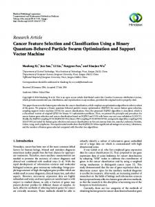
Figure 1: Block diagram to convert malware binary to an image N = 1 Sub-band . . .
. . . Sub-band
Image . . .
. . .
16-D Feature . . . 16-D Feature . . .
320-D Feature
N = 20 Sub-band
16-D Feature
Figure 2: Block diagram to compute texture feature on an image The matrix is then saved as an image and the process is shown in Figure 1.
2.2
Texture Feature Extraction
Once the malware binary is converted to an image, a texture based feature is computed on the image to characterize the malware. The texture feature that we use is the GIST feature [18], which is commonly used in image recognition systems such as scene classification and object recognition [25] and large scale image search[8]. We will briefly review the computation of the GIST feature vector. A more detailed explanation can be found in [25, 18]. Figure 2 shows the block diagram to obtain the GIST feature. Every image location is represented by the output of filters tuned to different orientations and scales. A steerable pyramid with 4 scales and 8 orientations is used. The local representation of an image is then given by: V L (x) = Vk (x)k=1..N where N = 20 is the number of sub-bands. In order to capture the global image properties while retaining some local information, the mean value of the magnitude of the local features is computed and averaged over large spatial regions: m(x) = x0 |V (x0 )|W (x0 − x) where W (x) is the averaging window. The resulting representation is downsampled to have a spatial resolution of M×M pixels (here we use M=4). Thus the feature vector obtained is of size M×M×N = 320. The steps to compute the texture feature are as follows:
P
1. Read every byte of a binary and store it in a numeric 1D array (range 0-255). 2. Convert the 1D array to a 2D array to obtain a grayscale image. The width of the image is fixed based on the file size of the binary[16]. 3. Reshape the image to a constant sized square image of size 64 × 64. 4. Compute a 16-dimensional texture feature across for N = 20 sub-bands. 5. Concatenate all the features to obtain a 320-dimensional feature vector.
2.3
Texture based Image Classification
Texture based image features are well known in classification of image categories. For example, in [25] GIST features are used
(a)
(b)
(c)
(d)
(e)
(f)
Figure 3: Sample images of 6 variants of: (a)Allaple, (b)Ejik, (c)Mydoom, (d)Tibs, (e)Udr, (f)Virut to classify outdoor scene categories. Their classification was performed using a k-nearest neighbors (k-NN) classifier, where a database of labeled scenes with the corresponding category called the training set is used to classify unlabeled scenes. Given a new scene, the k nearest neighbors are computed and these correspond to k scenes from the training set with the smallest distance to the test scene. Then the new scene is assigned the label of the scene category that is most represented within the k nearest neighbors. We use a similar approach, except that instead of outdoor scene categories, out categories correspond to malware families. The training set contains families of known malware. Each family further contain several malware variants. The 320-dimensional GIST features are computed for all the binaries in the training set. The following algorithm is used to classify a new unknown malware: 1. The 320-dimensional GIST feature vector is computed on the unknown malware binary. 2. The Euclidean Distance is computed with all feature vectors in the training set. 3. The nearest neighbors are the top k malware in the training set that have the smallest distance to the unknown. 4. The unknown malware is assigned a label that matches a majority returned by the k labels.
3.
DYNAMIC FEATURE EXTRACTION
In dynamic analysis, the behavior of the malware is traced by running the malware executable in a sandbox environment for several minutes. Based on the sandbox system under consideration, the type and granularity of data that is recorded might be different. In this paper, we evaluate two different dynamic analysis approaches. The first and commonly used appraoch is system-call level monitoring which might be implemented using API hooking or VM introspection. The system generates a sequential report of the monitored behavior for each binary, based on the performed operations and actions. The report typically includes all system calls and their arguments stored in a representation specifically tailored to behavior-based analysis.
Table 1: Malware datasets Dataset Host-Rx Reference Dataset Host-Rx Application Dataset Malhuer Reference Dataset Malheur Application Dataset VXHeavens Dataset
Num Binaries 393 2,140 3,131 33,698 63,002
Num Families 6 24 531
The second approach, which we call forensic snapshot comparison relies on a combination of features that are based on comparing the pre-infection and post-infection system snapshots. Some of the key features collected include AUTORUN ENTRIES, CONNECTION PORTS, DNS RECORDS, DROP FILES, PROCESS CHANGES, MUTEXES, THREAD COUNTS, and REGISTRY MODS. A whitelisting process is used to weigh down certain commonly occurring attribute values for filenames and DNS entries. A key difference between system-call monitoring and forensic comparison, is that the latter approach does not capture the temporal ordering of forensic events. The advantage is that it is simpler to implement and prioritize events that are deemed to be most interesting. To identify deterministic and non-deterministic features, each malware is executed three different times on different virtual machines and a JSON object is generated describing the malware behavior in each execution [32]. Depending on the presence of the key features, a binary feature vector is generated from the JSON object. If a key feature is present in the JSON object, then corresponding component in the feature vector is 1; otherwise the component is 0. The size of the feature vector depends on the diversity of the behavior of the malware corpus, but various between 6002000 for datasets used in this paper.
4.
EXPERIMENTS
In this section we present several experiments that compare the results of the binary texture analysis strategy against datasets analyzed in three separate malware binary classification efforts. In each experiment, every malware binary is characterized by a feature vector. We then use k-nearest neighbors (k-NN) with Euclidean distance measure for classification. The feature vectors are com-
puted for all binaries in the datasets and are divided into a training set and a testing set. For every feature vector in the testing set, the k-nearest neighbors in the training set are obtained. Then the vector is classified to the class which is the mode of its k-nearest neighbors. For all tests, we do a 10-fold cross validation, where under each test, a random subset of a class is used for training and testing. For each iteration, this test randomly selects 90% data from a class for training and 10% for testing. We summarize our datasets in Table 1. In the first experiment, Section 4.1, we compare binary texture analysis against a 2140 sample dataset. Out of this 2140, we downselected 393 binaries that have consistent labels and sufficient membership. We call this subset the Host-Rx reference dataset which was classified using a dynamic analysis technique where the binaries are clustered based on their observed forensic impacts on the host [32]. These clusters are also examined against antivirus labels, and the minimum family sample size is 20. We employed both image analysis and dynamic analysis on the Host-Rx dataset, recomputing the dynamic features and comparing the classification performance, since clustering is mainly focused in [32]. The average classification accuracy is 98% and 95% for dynamic and image analysis, respectively. Thus, we find the binary texture technique achieves comparable success but is able to complete its feature analysis in approximately 1/4000 the time required per binary. In the second experiment, we examine the Malhuer dataset, which was originally classified based on features derived by dynamic system call interception, as presented in [21]. These execution traces were converted to a Malware Instruction Set (MIST) format, from which feature vectors were extracted to effectively characterize the binaries. Since [21] already reports the results of a malware classification based on these features, we do not repeat the dynamic analysis. In Section 4.2, we present a comparative assessment of the Malheur dataset, which includes both a reference data set of 3131 malware binaries comprising 24 unique malware families, and an application dataset of roughly 33 thousand binaries that range from malicious, to unknown, to known benign. Using these datasets, we found that binary-texture classification produced comparable accuracies in both datasets, ranging from 97% for the reference set, to 86% accuracy for the application set. Finally, we present a larger experiment using a VX Heavens dataset consisting of a corpus of over 63 thousand malicious binaries comprising 531 unique families (as labeled by the Microsoft Security Essentials tool suite). Section 4.3 presents our results from the VX Heavens corpus, which was previously classified using the results from antivirus labels. Here the binary-texturing analysis produced a 72% match with the original Microsoft AV labels. However, while this result may appear lower than the previous experiments, we discuss issues in the labeling and our conservative interpretation of our binary-texture results, which we believe account for these results.
4.1
Experiment 1: Binary Texture Analysis vs Host-Rx Dynamic Analysis Dataset
In this experiment, we compute the feature vectors for binarytexture analysis and forensic dump-based dynamic analysis. We use the Host-RX dataset [32], for this comparison. The following process was used to select malware instances with reliable labels. The initial malware corpus consisted of 2140 malware binaries. The AV labels for these binaries were obtained from Virustotal.com [3]. Six AV vendors were used: AVG, AntiVir, BitDefender, Ikarus, Kaspersky and Microsoft. We attribute a label to a malware instance if at least 2 AV vendors share similar labels. Out of 2140 instances, only 450 malware samples had consistent labels. However, some malware families had very few samples. To conduct a meaningful (representative) analysis of the features collected, each family should have a large enough group of exem-
Table 2: Family/packer summary: Host-Rx reference dataset Family Allaple Ejik Mydoom Tibs Udr Virut
Total 81 30 151 31 34 66
Packed 3 11 124 0 34 3
Packer UPX 10 PeC, 1 nsPack UPX AsPack UPX
2 1.5 1 0.5 0
Allaple Ejik Mydoom Tibs Udr Virut
−0.5 −1 −1.5 −2
10 8
−2.5 6 −3 2
4 2 0
−2
0 −4
−6
−2 −8
−10
−4
Figure 5: Lower dimensional visualization of dynamic features on Host-Rx dataset plars from which to derive consistent features. For consistency with previous classification research ([21]) that is compared in the next section, we chose to remove families with less than 20 samples, and compiled a final collection of 393 malware binaries. These binaries (shown in Table 2) represented 6 malware families. We also check if these malware are packed or not using PeID and report the labels in Table 2. However, some of the malware that PeID did not detect could also be packed. Some images of the variants of the 6 families are shown in Figure 3
4.1.1
Dynamic Analysis Features
The dynamic analysis features are obtained from the forensic memory dumps and then converted to a vectorial form to produce a 651 dimensional vector for every malware instance, as shown in Figure 4. The result is a binary matrix, where 1 refers to the presence of a corresponding feature. The first 81 samples belong to Allaple and most of their features are between 75 and 219 (Figure 4). Similarly, we observe that other families like Ejik, Mydoom, Tibs, Udr and Virut have features concentrated in different sections of the feature matrix. For better visualization, these 651 dimensional features are projected to a lower dimensional space using multidimensional scaling [2]. As shown in Figure 5, the 6 families cluster well. To further validate the dynamic features, we classify the malware using a k-NN based classification across a 10-fold cross validation. For k=3, we obtain an average classification accuracy of 0.9822. As shown in Table 3, 387 out of 394 samples get classified correctly. Four samples of Virut are misclassified as Allaple due to feature similarity with that of Allaple (Figure 4).
4.1.2
Binary Image Features
Every malware binary is converted to an image and the GIST feature is computed. Hence every malware is characterized as a 320 dimensional vector which is based on the texture of the malware image. Figure 6 illustrates a lower dimensional visualization
Feature Matrix (0−white, 1−black)
Allaple 50 Ejik 100
File Number
150 Mydoom
200
250 Tibs 300
Udr
350
Virut
100
200
300 400 Feature Dimension (650)
500
600
Figure 4: Feature matrix of dynamic analysis features on Host-Rx dataset
Table 3: Confusion matrix for dynamic features on Host-Rx dataset
Allaple Ejik Mydoom Tibs Udr Virut
1 0.8 0.6
Allaple Ejik Mydoom Tibs Udr Virut
Allaple 81 0 0 0 0 0
Ejik 0 30 0 0 0 0
Mydoom 0 1 150 0 0 0
Tibs 0 1 0 30 0 0
Udr 0 0 0 0 34 0
Virut 4 1 0 0 0 61
0.4 0.2 0 −0.2 −0.4 −0.6 0.5
Table 4: Confusion matrix for binary image features on HostRx dataset
2.5
0
2 1.5 1
−0.5
0.5 0
Allaple Ejik Mydoom Tibs Udr Virut
Allaple 74 0 0 0 0 7
Ejik 0 30 0 0 0 0
Mydoom 0 0 151 0 0 0
Tibs 0 0 0 30 0 1
Udr 0 0 0 0 34 0
Virut 4 2 2 4 0 54
of the static features. Some malware families, such as Ejik, Allaple, Udr and Tibs, are tightly clustered. Mydoom exhibits an interesting pattern, where three sub-clusters emerge, and each is tightly formed. We manually analyzed each sub-cluster of Mydoom and found that the first sub-cluster had 124 samples, all of which were packed using UPX. The second and third sub-clusters had 15 and 12 members, respectively, but the images inside these sub-clusters appeared similar among themselves but different from the images of other sub-clusters. In contrast to the other families, the Virut family was not tightly clustered, as most images of the Virut family were found to be dissimilar. Similar to dynamic analysis, we performed a k-NN based classification across a 10-fold cross validation using the image based features. For k=3, we obtained an average classification accuracy of 0.9514. The confusion matrix is shown in Table 4. Except for Allaple and Virut families, almost all samples of the other four families were accurately classified.
4.1.3
Performance
−1
−0.5 −1
Figure 6: Lower dimensional visualization of binary texture features on Host-Rx dataset
Size of training set: We evaluate static and dynamic analysis by varying the number of training samples. We fix k = 3. The test is repeated three times and the average classification accuracy is obtained for each test, and then average again. Figure 7(a) illustrates that the dynamic features outperform the static features when the number of training samples are fewer (10%, 30%). Using 50% 90% training samples, the difference is only marginal. Varying k: Next, we fix the percentage of training samples at 50% per family and explore the impact of varying k. Similar to the previous test, the dynamic features are better at higher values of k (Figure 7(b), but there is only a marginal difference at lower values of k. This is also evident from Figure 5, where we see that the dynamic features are more tightly clustered when compared to the static features (Figure 6). Computation Time: The primary advantage of binary image features is the computation time. Since, our texture-based features are a direct abstraction of the raw binaries and do not require disassembly, the time to compute these features are considerably lower. We used an unoptimized Matlab implementation to compute the GIST features ([1]) on an Intel(R) Core(TM) i7 CPU running Windows 7
1
1
0.9
0.9 Texture Features Dynamic Features
0.7
0.7
0.6
0.6
0.5
0.5
0.4
0.4
0.3
0.3
0.2
0.2
0.1
0.1
0 10
20
30
40 50 60 Training Percentage
70
80
Texture Features Dynamic Features
0.8
Accuracy
Accuracy
0.8
90
0
1
2
3
(a)
4
5 k
6
7
8
9
(b)
Figure 7: Comparing classification accuracies of texture-based features and dynamic analysis features by varying: (a) number of training samples, (b) k nearest neighbors on Host-Rx Dataset
Table 5: Average computation time Dynamic Feature 4 mins
Static Feature 60 ms
(a) operating system. The average time to convert a malware binary to an image and compute the GIST features was 60 ms. In contrast, the average time required to obtain dynamic features from the same binary was 4 minutes. As shown in Table 5, the texture features are about 4000 times faster.
4.2
Experiment 2: Binary Texture Analysis vs Malheur Dynamic Analysis Dataset
For further validation, we compare binary-texture analysis to another dynamic analysis technique that derives its features from system call intercepts [21]. Here, we employ the Malheur dataset, which includes both a reference dataset and an application dataset. We obtained both dataset and classification results from the researchers who performed a dynamic analysis using this corpus [21]. We do not repeat their dynamic analysis here, but rather focus on performing a binary-texture analysis on this dataset, and then compare results from both methods. The Malheur [21] reference dataset consists of 3131 malware binaries from instances of 24 malware families. The malware binaries were labeled such that a majority amongst six different antivirus products shared similar labels. Further, in order to compensate for skewed distribution of samples per family, the authors of [21] discarded families less than 20 samples, and restricted the maximum samples per family to 300. The exact number of samples per family and the number of malware packed are given in Table 6. Once again we identify the packers using PeID. Although it is known that PeID could sometimes miss some packers, we still go with these labels. For the binary-texture analysis, we repeated the experiments by converting these malware to images, computing the image features and then classifying them using k-NN based classification. Initially, we do a 10-fold cross validation: the confusion matrix is shown in Figure 8(a). We obtained an average classification accuracy of 0.9757. In [21], the authors obtained similar results using dynamic analysis. From Table 6, we see that many families are packed, and some families such as Adultbrowser, Casino, Mag-
(b)
(c)
(d)
Figure 9: Images of malware binaries packed with UPX belonging to (a)Adultbrowser, (b)Casino, (c)Flystudio, (d)Magiccasino
iccasino and Podnhua, are all packed using the same packer, viz. UPX. A popular misconception is that if two binaries belonging to different families are packed using the same packer, then the two binaries are going to appear similar. In Figure 9, we can see that the images of malware binaries belonging to different families but packed with the same packer are indeed different. Instead of doing 10-fold cross validation, we randomly chose 10% of the samples from each family for training and the rest for testing. This was repeated multiple times. The average classification accuracy only dropped to 0.9130 and the confusion matrix is shown in Figure 8(b).
4.2.1
Malheur Application Dataset
The Malheur application dataset consists of unknown binaries obtained over a period of seven consecutive days from AV vendor Sunbelt Software. We received a total of 33,698 binaries. However, the authors of [21] labeled these using Kaspersky Antivirus. Out of 33,698 binaries, 7612 were labeled as ’unknown’. The authors mention that these are a set of benign executables. In performing binary-texture analysis on the Application Dataset, we retained the same labels given by the authors of [21]. Figure 10(a) shows the confusion matrix we obtained. The row with maximum confusion corresponds to the set of Nothing Found as mentioned in [21]. This set consisted of 7,622 binaries and were labeled as being “benign” in [21]. However, when we scanned these binaries using Microsoft Security Essentials, 3,393 binaries were flagged as malicious (our experiments also confirm this). We then repeated the experiment by not considering this mixed set. We obtained an average classification accuracy of 0.8615 (Figure 10(b)).
(a) (b) Figure 8: Confusion matrix obtained on Malheur Reference dataset using: (a) 10-fold cross validation, (b) 10% training sample 10
10
20
20
30
30
40
40
50
50
60
60
10
20
30
40
50
60
10
20
30
40
50
60
(a) (b) Figure 10: Confusion matrix on the: (a)Malheur Application data, (b)Malheur Application data without “benign” executables.
4.3
Table 6: Family/packer summary: Malheur Reference dataset Family Adultbrowser Allaple Bancos Casino Dorfdo Ejik Flystudio Ldpinch Looper Magiccasino Podnhua Poison Porndialer Rbot Rotator Sality Spygames Swizzor Vapsup Viking_dll Viking_dz Virut Woikoiner Zhelatin
Total 262 300 48 140 65 168 32 43 209 174 300 26 97 101 300 84 139 78 45 158 58 202 50 41
Packed 262 0 0 140 0 168 2 0 209 174 300 25 0 0 0 0 0 0 0 0 58 0 0 0
Packer UPX UPX PECompact UPX Aspack UPX UPX PEncrypt FSG -
Large Scale Analysis on VX-Heavens Application Dataset
We performed a binary-texture analysis on a larger corpus, consisting of 63,002 malware from 531 families (as labeled by Microsoft Security Essentials). These malware were obtained from VX-Heavens [4]. The results are shown in Figure 11. The average classification accuracy we obtained was 0.728. 33 families were classified with an accuracy of 1. Some of these include Skintrim.N, Yuner.A, Rootkit.AFE, Autorun.K, Adrotator. A total of 105 families fell above 90% accuracy, including Vake.H, Lolyda.AT, Seimon.D, Swizzor.gen!I, Azero.A, Allaple.A, Alueron.d, Instantaccess, Dialplatform, Jhee.V, Startpage.DE, to name a few. The families with high classification accuracies are those for which the variants appear visually similar. However, there are also families with low classification accuracies. 23 families had classification less than 0.1. These comprised a total of 1061 binaries (about 1.6% of the dataset). Some example families include Orsam.RTS, Koutodoor.A, Adrotator.A, Startpage, Kerproc.RTS. The lower accuracy in certain families arises mainly due to two reasons. The first is due to the visual dissimilarity of images in families such as Orsam.RTS, Kerproc.RTS. This dissimilarity could be due to a disparity of the labeling scheme (unlike our other experiments, our labels here are derived from one AV source). The second reason is because some families such as Startpage were classified as Starpage.DE or Startpage.E, which presumably imply that are variants derived from the same family). This is not completely incorrect since there is only a misclassification in the subscript and not on the family name. However, for completeness we still present these discrepancies as misclassification in our results, as we treat Microsoft’s labels Startpage, Startpage.DE, and Startpage.E as three separate families under our analysis.
4.4
Large Scale Analysis on Anubis Dataset
We also performed texture analysis on 685,490 malware binaries which we obtained from the authors of [6]. These malware were
50
100
150
200
250
300
350
400
450
500 50
100
150
200
250
300
350
400
450
500
Figure 11: Large scale analysis with confusion matrix for 63,002 malware comprising 531 families further clustered into 1441 behavioral clusters using the clustering technique proposed in [6] and we were given the cluster labels. We used these labels as the ground truth and performed k-NN based supervised classification with 10-fold cross validation to obtain a classification accuracy of 0.718. In other words, close to 500,000 malware inside the behavioral clusters are visually similar. This further reinforces that binary texture analysis is comparable with dynamic analysis even on a large malware corpus. 1
5. DISCUSSION In this section, we explore reasons behind why binary texture analysis provides useful results for classification despite the prevalence of packers and other obfuscators. Binary texture analysis leverages the fact that variants belonging to a common family have visual similarity (Figure 3). Binary packing systems do indeed change the structure of a binary, causing some amount of disruption to the visual similarity between the original packed and unpacked binary. However, we find that packed variants belonging to a common malware family continue to exhibit visual similarity with one another. We discuss some of our observations below: Observation 1: While packers do their best to increase to computational effort required to reverse engineer the original source object code, they are currently not designed to produce fully nondeterministic binary restructuring across the packed binary. Rather, a given packer conducts binary transformations that may in some cases be easily observable across a common source binary (e.g, output file size, number of code and data sections, and their respective sizes), as well as some transformations that are not as obvious. For example, the use of fixed size encryption keys (e.g., XOR keys) commonly used by many packers result in predictable repeating patterns as they transform the original object code. This explains why malware belonging to different families are still distinguishable (Figure 9), even after being repeatedly packed by the same packer. Observation 2: From our datasets, we find that a single malware family is rarely packed with more than one or two packers (Table 2, Table 6). Since we used supervised learning and classification, our technique can accurately deal with scenarios where the same malware is packed with multiple packers. As long as the packers used in the testing set are also present in the training set to obfuscate the malware family, we may remain agnostic to whether or not a malware distributor chooses to employ multiple packers. Observation 3: The use of a specific version of a packer and a 1 This experiment was not included in the original paper due to shortage of time
set of options by itself helps to narrow down a malware sample to a handful of families. We can further narrow common samples down based on their packed file size and other attributes such as sizes of respective sections. Many malware families implement custom encryption or obfuscation schemes which makes their identification easier. Observation 4: Finally, in any malware corpus, there is a fraction of malware that is unpacked. Notwithstanding the above observations, the texture-based classification scheme is still vulnerable to knowledgeable adversaries who explicitly obfuscate their malware to defeat texture analysis. Regardless, our experimental results suggest it could be a very useful technique in dealing with contemporary malware. When combined with sampling and dynamic analysis, texture-based classification could prove to dramatically accelerate the efficiency of automated malware classification systems for a wide-range of malware samples.
6.
RELATED WORK
Malware classification is an important problem that has attracted considerable attention. Several techniques have been proposed on malware clustering [6, 5, 31, 21, 14, 10, 29], classification [13, 20, 21, 9, 12, 19] and similarity [11, 27, 7, 28]. We review some of them below. Dynamic analysis-based classification techniques. Of particular relevance are recent efforts that have tried to develop models for classifying malware based on dynamic analysis. Several tools exist for sandboxed execution of malware including CWSandbox [30], Norman Sandbox [17], and TTanalyze [26]. While CWSandbox and TTanalyze leverage API hooking, Norman Sandbox implements a simulated Windows environment for analyzing malware. A complementary analysis is proposed in [15], where a layered architecture is proposed for building abstract models based on run-time system call monitoring of programs. Bailey et al. were among the first to point out inconsistencies in labeling by popular AV vendors and present an automated classification system as a solution for robustly classifying malware binaries through offline behavioral analysis [5]. Another related work is from Kolbitsch et al. [12], where dynamic analysis is used to build models of malware programs based on information flow between system calls. Similarly, Bayer et al. [6] propose an unsupervised learning system to automatically cluster malware based on their behavioral profile. From a random sample of 14,212 malware, they selected samples for which the majority of six different antivirus scanners reported the same family to result in a total of 2,658 samples comprising 84 families. They obtained a surprisingly high precision and recall on those samples and also showed great improvements in time when compared to previous approaches. However, Li et al., in a recent paper [14] showed that the high precision and recall of the above technique is due to selection bias in generating their ground truth. Rieck et al. propose a supervised learning approach to behaviorbased malware classification [20]. They use a labeled dataset of 10,072 malware samples comprising 14 families. The behavior of the samples is monitored in a sandbox environment from which behavioral reports are generated. From every report, they generate feature vectors based on the frequency of some specific strings. Finally, they use a Support Vector Machines for classification. In [21], they extend this technique and build a system which combines both classification and clustering. Our motivation and approach is most similar to their work, with the key exception that we rely on statically-derived features, i.e., binary texture for our classification. Our results on their dataset show that we can generate comparable results by simply relying on image based features. Static feature-based classification techniques. Our work is not
[7] E. Carrera and G. Erdelyi. Digital genome mapping and advanced binary malware analysis. In Proceedings of Virus Bulletin Conference, 2004. [8] M. Douze, H. Jegou, H. Sandhawalia, L. Amsaleg, and C. Schmid. Evaluation of gist descriptors fro web-scale image search. In Proceedings of CIVR, 2009. [9] X. Hu, T. cker Chiueh, and K. G. Shin. Large-scale malware indexing using function-call graphs. In Proceedings of CCS, 2009. [10] J. Jang, D. Brumley, and S. Venkataraman. Bitshred: Fast, scalable malware triage. Technical report, Cylab, Carnegie Mellon University, 2010. [11] E. Karim, A. Walenstein, and A. Lakhotia. Malware phylogeny generation using permutations of code. European Research Journal on Computer Virology, 1(2), November 2005. 7. CONCLUSIONS [12] C. Kolbitsch, P. M. Comparetti, C. Kruegel, E. Kirda, Our paper provides a comparitive assessement of automated behaviorX. Zhou, and X. Wang. Effective and efficient malware based classification techniques with a newly proposed static techdetection at the end host. In Proceedings of Usenix Security, nique for binary classification that is based on image texture analy2009. sis. We compare the two classification strategies based on two dif[13] T. Lee and J. Mody. Behavioral classification. In EICAR, ferent datasets: Host-Rx dataset and Malheur dataset. We find that 2006. supervised classification technique based on simple texture analysis [14] P. Li, L. Liu, D. Gao, and M. K. Reiter. On challenges in can be performed highly scalably and is comparable to contempoevaluating malware clustering. In Proceedings of RAID, rary dynamic analysis in its accuracy (over 97% on dataset with 2010. consistent labeling). Surprisingly, this approach also seems to be [15] L. Martignoni, E. Stinson, M. Fredrikson, S. Jha, and resilient to contemporary packing strategies and can robustly clasJ. Mitchell. A layered architecture for detecting malicious sify large corpus of malware with both packed and unpacked sambehaviors. In Proceedings of RAID, 2008. ples. Finally, we validate the texture-based classification scheme on a large scale dataset of over 60K binaries where we find over [16] L. Nataraj, S. Karthikeyan, G. Jacob, and B. Manjunath. 72% consistency when compared with labels from one AV vendor Malware images: Visualization and autmoatic classification. and also on a larger corpus of over 685K malware where we are In Proceedings of VizSec, 2011. close to 72% consistent with the behavioral cluster labels. [17] Norman Sandbox. http://sandbox.norman.no. Our results demonstrate that static classification techniques, such [18] A. Olivia and A. Torralba. Modeling the shape of a scene: a as texture analysis, could be a useful complement to dynamic analholistic representation of the spatial envelope. Intl. Journal ysis and an effective preprocessing step in a scalable next-generation of Computer Vision, 42(3):145–175, 2001. malware classification system. [19] Y. Park, D. Reeves, V. Mulukutla, and B. Sundaravel. Fast malware classification by automated behavioral graph matching. In Proceedings of CSIIRW, 2010. 8. ACKNOWLEDGMENTS [20] K. Rieck, T. Holz, C. Willems, P. Dussel, and P. Laskov. We would like to thank the authors of [21] for providing us Learning and classification of malware behavior. In the dataset used in their paper. This material is based upon work Proceedings of DIMVA, 2008. supported through the U.S. Army Research Office (ARO) under [21] K. Rieck, P. Trinius, C. Willems, and T. Holz. Automatic the Cyber- TA Research Grant No.W911NF-06-1-0316 and Grant analysis of malware behavior using machine learning. W911NF0610042, and by the National Science Foundation under Technical report, University of Mannheim, 2009. Grant IIS-0905518, and by the Office of Naval Research under the [22] M. Sharif, A. Lanzi, J. Giffin, and W. Lee. Impeding grant ONR # N00014-11-10111. Any opinions, findings, and conmalware analysis using conditional code obfuscation. In clusions or recommendations expressed in this material are those Proceedings of NDSS, 2008. of the author(s) and do not necessarily reflect the views of U.S. [23] D. Takahashi. Symantec identified 286m malware threats in ARO or the National Science Foundation or the Office of Naval 2010. http://venturebeat.com/2011/04/04/symantecResearch. identified-286m-malware-threats-in-2010/, 2010. 9. REFERENCES [24] R. Tian, L. Batten, R. Islam, and S. Versteeg. An automated classification system based on strings and of trojan and virus [1] GIST Code. http://people.csail.mit.edu/torralba/code/spatialenvelope. families. In Proceedings of MALWARE, 2009. [2] Multi-dimensional Scaling, DR Toolbox. [25] A. Torralba, K. Murphy, W. Freeman, and M. Rubin. http://homepage.tudelft.nl/19j49/. Context-based vision systems for place and object [3] Virustotal.com. http://www.virustotal.com. recognition. In Proceedings of ICCV, 2003. [4] VX Heavens. http://vx.netlux.org. [26] U.Bayer, C.Kruegel, and E.Kirda. Ttanalyze: A tool for [5] M. Bailey, J. Oberheide, J. Andersen, Z. Mao, and analyzing malware. In EICAR, 2006. F. Jahanian. Automated classification and analysis of internet [27] A. Walenstein, M. Hayes, and A. Lakhotia. Phylogenetic malware. In RAID, 2007. Comparisons of Malware. Virus Bulletin Conference, 2007. [6] U. Bayer, P. M. Comparetti, C. Hlauschek, C. Kruegel, and [28] S. Wehner. Analyzing worms and network traffic using E. Kirda. Scalable, behavior-based malware clustering. In Proceedings of NDSS, 2009. the first to attempt static feature-based malware classification. Prior work has looked at classification based on graph structures on disassemblies as well as visible structures from PE header and binary strings. Karim et al. examine the problem of developing phylogenetic models for detecting malware that evolves through code permutations [11, 27]. Carrera et al. develop a taxonomy of malware using graph-based representation and comparison techniques for malware [7]. In [19], Park et al. classify malware based on detecting the maximal common sub-graph in a behavioral graph and demonstrate their results on a corpus of 300 malware comprising 6 families. Tian et al. [24] use printable strings in the malware for classification. Our work differs from prior attempts on staticfeature based classification in our use of binary texture analysis as a means for malware classification.
[29] [30]
[31]
[32]
compression. Journal of Computer Security, 15(3):303–320, 2007. G. Wicherski. pehash: A novel approach to fast malware clustering. In Proceedings of LEET, 2009. C. Willems, T. Holz, and F. Freiling. Toward automated dynamic malware analysis using cwsandbox. IEEE Security and Privacy (Vol. 5, No. 2), March/April 2007. Y. Ye, T. Li, Y. Chen, and Q. Jiang. Automatic malware categorization using cluster ensemble. In Proceedings of KDD, 2010. J. Zhang, P. Porras, and V. Yegneswaran. Host-rx: Automated malware diagnosis based on probabilistic behavior models. Technical report, SRI International, 2009.