Proceedings of the 17th Iranian Conference of Biomedical Engineering (ICBME2010), 3-4 November 2010
A comparison between new L 1 minimization algorithms in Electrical Impedance Tomography using the Pareto Curve Jouhin Nasehi Tehrani The University of Sydney The school of Electrical and information Engineering Sydney, Australia
[email protected]
Alistair McEwan The University of Sydney The school of Electrical and information Engineering Sydney, Australia
[email protected]
Abstract- Electrical Impedance Tomography (EIT) calculates the
internal
electrical
conductivity contact
distribution
within
measurements.
a
body
using
Conventional
EIT
reconstruction methods solve a linear model by minimizing the least
squares
error,
i.e.,
the
Euclidian
or
L2-norm,
with
regularization. Recently, total variation and Ll regularization have become more popular in medical image reconstruction. Here, we introduce new method for evaluating and finding the regularization Frontier
parameters
curve).
This
by
method
using traces
the the
Ll-curve optimal
(Pareto trade-off
between the least-squares fit of residual and the Ll-norm of the solution. In this paper, we compare this algorithm with two Ll norm regularization methods. The results show that this method can help us to have more control on filtering and sparsity of the solution.
It
also shows that visualizing the Ll-curve (Pareto
Curve) in order to understand the trade-offs between the norms of the residual and the solution can be helpful in situation where we do not have a very good estimation about the level of the noise.
Keywords- Image reconstruction; regularization; Electrical Impedance Tomography; Pareto Curve
I.
INTRODUCTION
Electrical Impedance Tomography (EIT) is an imaging method using applied current and voltage measurement around the medium of interest. The internal impedance changes are found by an image reconstruction algorithm that takes into account prior information such as electrode locations, external and internal boundaries, and contact impedance. However, even with this information the images are limited in spatial resolution due to the ill-posed nature of the problem, i.e., the large number of unknowns compared to the number of independent measurements. Most EIT reconstruction methods consider a linear model of the form:
( 1)
b =}x +n
For EIT, x E IR\.N is a vector of values representing the change in the conductivity within the medium, b E IR\.M is the vector of the observed voltage measurements, ] E IR\.MXN is the
Jacobian matrix, relating voltage changes to conductivity changes via the reciprocity principle[1], and n is the noise in the measurements. The noise arises from multiple sources, such as RF coupling onto signal wires, electrode malfunction, and subject movement artifacts [2]. In this paper the noise is modeled as Gaussian noise despite the fact that it may not be exactly Gaussian distributed. In practice, noise sources can introduce more outliers than a Gaussian model would predict. The medium is commonly modeled as a finite element mesh (FEM). There are N=1600 impedance elements in our FEM model and M is the number of voltage measurements. In our 16 electrode system two adjacent electrodes are used for current injection. With the remaining 14 electrodes we measure 13 voltage differences between adjacent electrodes. The current injection site sequentially changes from one electrode position to the next, so M is equal to 16 x 13 208. As M « N the system is under-determined and there exist infinitely many solutions. Minimizing the L2-norm using Tikhonov regularization [3] is a standard technique for solving such an underdetermined problem: =
min IlJx
-
b"� + A "x"� ,
(2)
Where IIxII2 denotes the L2-norm of x and A > 0 is the regularization parameter. Conventional EIT uses gradient descent, steepest descent, Newton, or Quasi-Newton methods to minimize the L2-norm. It is also common to use a Pareto efficiency trade-off curve called the L-curve (or L2-curve) where the optimal trade-off points of the objective function and regularisation term are plotted. The knee or corner of this curve is detected by the derivative and used to find an optimal regularisation parameter. These methods result in smooth EIT images. The application of non-smooth reconstruction techniques is important for medical imaging because one aims to extract discontinuous profiles[4, 5]. One technique to permit image regularization without imposing smoothing is the Total Variation (TV)[6]. In this paper we implement new technique for finding the regularization parameters by using the Ll-curve (Pareto Curve). We perform the least absolute
This work was supported by an Australian government Postgraduate Award (APA).
978-1-4244-7484-4/10/$26.00 ©2010 IEEE
shrinkage and selection operator (LASSO) [7] and the related method of basis pursuit denoising (BPDN)[8]. The iterative points on the Pareto Curve are the shared solution of these two algorithms which defines the optimal trade-off between the two-norm of the residual and the one-norm of the solution. Hence the LI-curve is also referred to as the Pareto Curve as it traces the Pareto efficient points. We compare the results with the following L1 minimization algorithms: (1) a specialized interior-point method for solving a large-scale LI-regularized least squares problem (LSP) that uses the preconditioned conjugate gradients (PCG) algorithm to compute the search direction[9). This method, termed LI-LS has been shown to be useful for magnetic resonance imaging [10, 11). (2) A new iterative shrinkage / thresholding [12] algorithm for Ll-norm regularized LSP (TWIST)[13). All The Matlab function calls used to simulate these algorithms can be found in [14] Appendix A. II.
REGULARIZAT10N ALGORITHMS
A. Newton interior-Point Method (Ll-LS)
For converting the L2-norm regularization to LI-norm the right side of the constraint changes to 11.111 of the solution as shown in equation (3).
min llb - lPslI� subject to IIslll
::;; k.
( 3)
However, the objective function shown in equation (3) is convex, but not differentiable, making it difficult to solve directly. It is possible to transform equation (3) to a convex quadratic problem with linear inequality constraints as follows:
min lllx - bll� + "-L�l Ui subject to -Ui ::;; X ::;; Ui' iE[l, n],
C. Lasso and BPDN algorithms
Lasso seeks a minimum LI-norm solution of an under determined least squares problem, which can be formulated as:
min lllx - bll� subject to IIxlll
min llxlll subject to IlJx - bll�
III.
(5)
where A is the regularization parameter and IIxll1 is the Ll norm of the conductivity changes[8).
(J
(7)
PARETO CURVE SOLUTION
This curve can trace the optimal trade-off between IIIx - b liz and IIxll1 for a specific pair of J and b in equation (1). At each iteration, a spectral gradient projection (SPG) method approximately minimizes a least square problem with an explicit one norm constraint. The optimal solution of Lasso for each value of T > 0 can be calculated by using Newton's method to find a root of the nonlinear equation lib - JXTII� = (J. Where XT(1 is a solution that causes Lasso (equation (5)) and Basis pursuit (equation (6)) shares the same solution. Figure 1 shows the Pareto Curve. This curve is continuously differentiable and convex. The residual of T-r is equal to b - ] X-r and decreases with increasing of T. Teon is the optimal objective value of the basis pursuit problem.
(0,11 b112) Slope
.,.D I
::