Received: 15 March 2017
Revised: 19 May 2017
Accepted: 19 May 2017
DOI: 10.1002/gepi.22061
RESEARCH ARTICLE
A comparison of methods for inferring causal relationships between genotype and phenotype using additional biological measurements Holly F. Ainsworth1
So-Youn Shin2
1 Institute of Genetic Medicine, Newcastle
University, International Centre for Life, Central Parkway, Newcastle upon Tyne, United Kingdom 2 MRC Integrative Epidemiology Unit (IEU),
University of Bristol, Bristol, United Kingdom Correspondence Heather J. Cordell, Institute of Genetic Medicine, Newcastle University, International Centre for Life, Central Parkway, Newcastle upon Tyne, NE1 3BZ, UK. Email:
[email protected]
Heather J. Cordell1
ABSTRACT Genome wide association studies (GWAS) have been very successful over the last decade at identifying genetic variants associated with disease phenotypes. However, interpretation of the results obtained can be challenging. Incorporation of further relevant biological measurements (e.g. ‘omics’ data) measured in the same individuals for whom we have genotype and phenotype data may help us to learn more about the mechanism and pathways through which causal genetic variants affect disease. We review various methods for causal inference that can be used for assessing the relationships between genetic variables, other biological measures, and phenotypic outcome, and present a simulation study assessing the performance of the methods under different conditions. In general, the methods we considered did well at inferring the causal structure for data simulated under simple scenarios. However, the presence of an unknown and unmeasured common environmental effect could lead to spurious inferences, with the methods we considered displaying varying degrees of robustness to this confounder. The use of causal inference techniques to integrate omics and GWAS data has the potential to improve biological understanding of the pathways leading to disease. Our study demonstrates the suitability of various methods for performing causal inference under several biologically plausible scenarios. KEYWORDS Bayesian networks, causal inference, Mendelian randomisation, structural equation modelling
1
I N T RO D U C T I O N
Many genetic variants associated with human diseases have been successfully identified using genome wide association studies (GWAS) (Visscher, Brown, McCarthy, & Yang, 2012). However, a typical GWAS provides limited further insight into the biological mechanism through which these genetic variants are implicated in disease. The variants implicated by GWAS are not necessarily true causal variants (that directly influence disease risk) but may rather correspond to variants in linkage disequilibrium with the causal variant(s). Even for
putative causal variants, there is typically a lack of understanding of how the identified genetic variants influence the phenotype at a molecular/cellular level. Consequently, moving towards therapeutic intervention is not straightforward. It has become popular to use data from publicly available databases to provide functional evidence for loci that have been identified through GWAS (Cordell et al., 2015; Wain et al., 2017; Warren et al., 2017). For example, it may be of interest to consider whether a single nucleotide polymorphism (SNP) associated with disease associates with gene expression in a relevant tissue. If such an association can be
This is an open access article under the terms of the Creative Commons Attribution License, which permits use, distribution and reproduction in any medium, provided the original work is properly cited. © 2017 The Authors Genetic Epidemiology Published by Wiley Periodicals, Inc. Genet. Epidemiol. 2017;1–10.
www.geneticepi.org
1
AINSWORTH ET AL.
2
demonstrated, it might indicate that the observed association between the SNP and disease phenotype is mediated through altering the level of gene expression. However, the individuals contributing to public databases are typically different from those who feature in the original GWAS data set (and the results may even derive from experiments on a different organism), making direct conclusions about causality problematic. We therefore consider instead the situation whereby we have measurements of a potential intermediate phenotype (such as gene expression) taken in the same set of individuals as are included in the GWAS data set. Use of such ‘overlapping’ sets of measurements allows us to address directly questions regarding the causal relationships between variables. This approach has been employed previously for examining the potential role of DNA methylation as a mediator between SNP genotype and rheumatoid arthritis (Liu et al., 2013) or ovarian cancer (Koestler et al., 2014), and for investigating the role of metabolites as a potential mediator between SNP genotype and various lipid traits (Shin et al., 2014). In these previous studies, a filtering step based on consideration of pairwise correlations/associations between variables of different types was first used in order to filter the number of variables considered to a manageable level, retaining only those variables whose pairwise correlations reached a specified level of significance. All resulting ‘triplets’ of variables (consisting of a genetic variable, a potential mediator variable such as a variable related to DNA methylation or metabolite concentration, and an outcome variable such as rheumatoid arthritis or a lipid trait) were then subjected to a causal inference test (CIT)—the CIT (Millstein, 2016; Millstein, Zhang, Zhu, & Schadt, 2009) in Liu et al. (2013), and Mendelian randomisation (Smith & Ebrahim, 2003) and structural equation modelling (Bollen, 1989) in Shin et al. (2014)—in order to elucidate the causal relationships between the variables in each triplet. Use of a similar pairwise filtering approach was employed by Zhu et al. (2016), who developed a method known as SMR (summary data-based Mendelian randomisation). SMR uses GWAS summary statistics (SNP effects) together with eQTL summary statistics from publicly available databases to test for association between predicted gene expression and phenotype, with a further test known as HEIDI (heterogeneity in dependent instruments) used to elucidate causal relationships between triplets of variables; in their application Zhu et al. (2016) restricted the HEIDI analysis to expression probes that (a) showed association at 𝑃 < 5 × 10⁻⁸ with nearby SNPs (so-called ciseQTLs) and (b) also showed association at 𝑃 < 8.4 × 10⁻⁶ with one of five complex traits considered. In an expanded version of this study, Pavlides et al. (2016) increased the number of phenotypes considered to 28 complex traits and diseases, while using the same filtering thresholds to focus the HEIDI analysis on 271 triplets of variables, each consisting of a SNP (cis-eQTL), its associated gene expression probe and
a complex trait with which the gene expression probe is also associated. More ambitiously, the (probabilistic) construction of entire causal networks of multiple variables, including metabolomic and transcriptomic (gene-expression) measurements, has been carried out using approaches based on Bayesian networks (Zhu et al., 2004, 2012). This approach allows in principle the simultaneous consideration of a potentially large number of variables. Bayesian networks can only be solved at the level of Markov (mathematically) equivalent structures; however genetic data can be incorporated in the network prior as ‘causal anchor’ to help direct the edges in the network. Although the Bayesian networks considered generally contain large numbers of variables, this incorporation of genetic data in order to help direct edges has typically involved calculations performed on smaller subunits such as triplets of variables (e.g., one genetic factor and a pair of nongenetic factors such as metabolite concentrations or gene expression values) (Zhu et al., 2004, 2012). The use of genetic data as a causal anchor for delineating the causal relationships between other variables (in particular between modifiable risk factors and phenotypic outcome) has a long history in the field of genetic epidemiology and has been popularised in the approach of Mendelian randomisation (Smith & Ebrahim, 2003) and its extensions (such as SMR, described above). Given the focus, thus far, in the literature, on using triplets of variables to perform causal inference, we were interested to examine the performance of the available methods in this simple situation, before moving to the more complex situation of analysing multiple variables (as are routinely encountered in modern ‘omics’ data sets) simultaneously. We chose to investigate the following methods for causal inference: Mendelian randomisation (Smith & Ebrahim, 2003), a CIT (Millstein, 2016; Millstein et al., 2009), structural equation modelling and several Bayesian methods. We present a simulation study that assesses the performance of the methods under different conditions, assuming throughout that we have genotype data along with two observed quantitative (continuous) phenotypes. We also consider how inference is affected by the presence of unmeasured environmental confounding factors. We begin by outlining the details of our simulation study before presenting an overview and discussion of the results.
2
M ETH O DS
For the purposes of our study, we assume we have genotype data (𝐺) from a single SNP, along with measurements of gene expression (𝑋) and a further phenotype of interest (𝑌 ). In reality, 𝑋 could be any omics measurement of interest (e.g., gene expression, DNA methylation, metabolite concentration, proteomic measurements etc.). We assume that it is known that there exist some pairwise associations between the variables;
AINSWORTH ET AL.
3
F I G U R E 1 Possible causal models explaining the relationship between a genetic variant 𝐺 and two observed traits 𝑋 and 𝑌 . Models (h)–(l) include an unmeasured common enviromental effect 𝐸
this could have been established during a preprocessing or filtering step. Figure 1 shows some hypothesised causal models to explain the relationship between the variables 𝐺, 𝑋, and 𝑌 . Where an arrow is present between two variables, this is indicative of a causal relationship between these variables, the direction is characterised by the direction of the arrow. The set of models is restricted to those that are biologically plausible, consequently we do not consider models in which the genetic variant 𝐺 can be influenced by any other variable. In models (h)–(l), we also include an unmeasured confounder corresponding to an environmental effect 𝐸. Given observed data on 𝐺, 𝑋, and 𝑌 , we were interested to explore how well the underlying causal structure can be learned. We consider several commonly used techniques for attempting to infer underlying causal structure between variables. We first consider two methods designed to detect causal associations in specific scenarios: Mendelian randomisation (MR) (Smith & Ebrahim, 2003) and a CIT (Millstein, 2016; Millstein et al., 2009). These methods are not designed for an exploratory analysis involving many structures and would normally only be used when there is a strong prior hypothesis that a particular causal model gave rise to the data. Nevertheless, we consider it useful to explore how well these methods perform on our simulated data sets. We also consider several approaches used for causal modelling that are more flexible, these are structural equation modelling (SEM) (Bollen,
1989; Fox, Nie, & Byrnes, 2015), a Bayesian unified framework (BUF) (Stephens, 2013), and two different R packages for learning Bayesian networks: DEAL (Bottcher & Dethlefsen, 2013) and BNLEARN (Scutari, 2010). A more detailed overview of all of these techniques is provided in the Supporting Information.
2.1
Simulation Study
For each of the 12 causal scenarios given in Figure 1, 1,000 replicate data sets were simulated, each containing 1,000 individuals. The SNP genotype data (𝐺) were generated assuming Hardy-Weinberg equilibrium and a minor allele frequency of 0.1. The direct effect sizes were initially chosen to be constant throughout all models. For example, when simulating data from model (a) in Figure 1, the effect size of 𝐺 on 𝑋 is the same as the effect size of 𝐺 on 𝑌 . Full details of the simulation models are given in Table 1. For each simulated data set, we applied each of the six causal inference methods under consideration. The idea was to assess how well these methods could recover the true underlying causal structure. Because the methods we consider approach the problem from different angles, direct comparison of results is not straightforward. MR and the CIT are designed to test for specific causal scenarios, usually informed by prior knowledge. In our setup, MR is designed to identify the causal relationship 𝑋 → 𝑌 while the CIT identifies that 𝑋 acts as a mediator between 𝐺 and 𝑌
AINSWORTH ET AL.
4
TABLE 1
Details of simulation models for scenarios given in Figure 1 Simulation model
Scenario
X
Y
(a)
2 𝑋|𝐺 ∼ 𝑁(𝜇𝑋 + 𝛼𝐺, 𝜎𝑋 )
𝑌 |𝐺 ∼ 𝑁(𝜇𝑌 + 𝛽𝐺, 𝜎𝑌2 )
(b)
2 𝑋|𝐺 ∼ 𝑁(𝜇𝑋 + 𝛼𝐺, 𝜎𝑋 )
𝑌 |𝑋 ∼ 𝑁(𝜇𝑌 + 𝛾𝑋, 𝜎𝑌2 )
(c)
2 𝑋|𝑌 ∼ 𝑁(𝜇𝑋 + 𝛾𝑌 , 𝜎𝑋 )
𝑌 |𝐺 ∼ 𝑁(𝜇𝑌 + 𝛽𝐺, 𝜎𝑌2 )
(d)
𝑋|𝐺 ∼ 𝑁(𝜇𝑋 + 𝛼𝐺,
2 𝜎𝑋 )
(e)
2 𝑋|𝐺, 𝑌 ∼ 𝑁(𝜇𝑋 + 𝛼𝐺 + 𝛿𝑌 , 𝜎𝑋 )
(f)
𝑋|𝐺, 𝑌 ∼ 𝑁(𝜇𝑋 + 𝛼𝐺 + 𝛿𝑌 ,
2 𝜎𝑋 )
(g)
2 𝑋 ∼ 𝑁(𝜇𝑋 , 𝜎𝑋 )
𝑋|𝐺, 𝐸 ∼ 𝑁(𝜇𝑋 + 𝛼𝐺 + 𝜁𝐸,
(i)
𝑋|𝐺, 𝐸 ∼ 𝑁(𝜇𝑋 + 𝛼𝐺 + 𝜁𝐸,
(j)
𝑋|𝑌 , 𝐸 ∼ 𝑁(𝜇𝑋 + 𝛿𝑌 + 𝜁𝐸,
(k)
𝑋|𝐺, 𝐸 ∼ 𝑁(𝜇𝑋 + 𝛼𝐺 + 𝜁𝐸, 𝑋|𝐸 ∼ 𝑁(𝜇𝑋 + 𝜁𝐸,
𝑌 |𝐺, 𝑋 ∼ 𝑁(𝜇𝑌 + 𝛽𝐺 + 𝛾𝑋, 𝜎𝑌2 ) 𝑌 |𝐺 ∼ 𝑁(𝜇𝑌 + 𝛽𝐺, 𝜎𝑌2 ) 𝑌 ∼ 𝑁(𝜇𝑌 , 𝜎𝑌2 ) 𝑌 |𝐺, 𝑋 ∼ 𝑁(𝜇𝑌 + 𝛽𝐺 + 𝛾𝑋, 𝜎𝑌2 )
(h)
(l)
E
2 𝜎𝑋 ) 2 𝜎𝑋 ) 2 𝜎𝑋 ) 2 𝜎𝑋 )
2 𝜎𝑋 )
𝑌 |𝐺, 𝐸 ∼ 𝑁(𝜇𝑌 + 𝛽𝐺 + 𝜁𝐸, 𝜎𝑌2 )
𝐸 ∼ 𝑁(0, 𝜎𝐸2 )
𝑌 |𝑋, 𝐸 ∼ 𝑁(𝜇𝑌 + 𝛾𝑋 + 𝜁𝐸, 𝜎𝑌2 )
𝐸 ∼ 𝑁(0, 𝜎𝐸2 )
𝜎𝑌2 )
𝐸 ∼ 𝑁(0, 𝜎𝐸2 )
𝑌 |𝐺, 𝐸 ∼ 𝑁(𝜇𝑌 + 𝛽𝐺 + 𝜁𝐸, 𝑌 |𝐸 ∼ 𝑁(𝜇𝑌 + 𝜁𝐸, 𝜎𝑌2 ) 𝑌 |𝐺, 𝐸 ∼ 𝑁(𝜇𝑌 + 𝛽𝐺 + 𝜁𝐸,
𝐸 ∼ 𝑁(0, 𝜎𝐸2 ) 𝜎𝑌2 )
𝐸 ∼ 𝑁(0, 𝜎𝐸2 )
The default parameter values are 𝛼= 1, 𝛽= 1, 𝛿= 1, 𝜇𝑋 = 10, 𝜇𝑌 = 10, 𝛾= 1, 𝜁= 1, 𝜎𝑋 = 0.3, 𝜎𝑌 = 0.3, 𝜎𝐸 = 0.3. G is coded as (0, 1, 2) according to the number of minor alleles present at the SNP
(i.e., identifies the relationship 𝐺 → 𝑋 → 𝑌 ) and, moreover, that 𝑋 is the only causal link between 𝐺 and 𝑌 . For MR and the CIT, we consider that the specified causal relationships have been established if a significant P-value (𝑃 < 0.05) is returned from the respective test. The other four methods are more flexible because they all consider a wider range of causal models. The Bayesian network methods (DEAL and BNLEARN) can consider the full space of models arising from three variables, including models (a)–(g) in Figure 1. However, they naturally exclude any models with an arrow going towards the SNP because the methods assume that discrete variables do not have continuous parents. This convenient feature of Bayesian networks automatically imposes the natural biological assumption that genetic factors (such as SNPs) are assigned at birth and will not be influenced by any other of the measured variables. The Bayesian network methods assign to each model a network score, and we consider the model with the highest network score to be the most plausible. For SEM, not all structures are considered as only a subset of models have enough degrees of freedom to be testable. These models are (a), (b), (c), (f) and (g) from Figure 1. We choose the model with the lowest Bayesian information criterion (BIC) (Schwarz, 1978) to be the most plausible. The BUF method considers all possible partitions of variables X and Y into three categories: 𝑈 (unassociated with 𝐺), 𝐷 (directly associated with 𝐺), and 𝐼 (indirectly associated with 𝐺). This gives a total of nine partitions. Of these nine partitions, three correspond to models in Figure 1, namely (a), (b), and (c). In the following, we will refer to two further partitions, (m) and (n), where (m) represents a model with just one arrow 𝐺 → 𝑋 and (n) represents a similar model with 𝐺 → 𝑌 . We take the model with the highest Bayes factor to be the most plausible.
3
RESULTS
Figure 2 shows the results of applying MR and the CIT to simulated data sets. In each plot, the 𝑥-axis indicates the scenario under which the data have been simulated, as illustrated in Figure 1. The 𝑦-axis represents the proportion of simulated data sets in which the test detects a specified causal relationship. This relationship is 𝑋 → 𝑌 for MR and 𝐺 → 𝑋 → 𝑌 (with no other causal link between 𝐺 and 𝑌 ) for the CIT. As expected, for data simulated under scenario (b), the causal structure can be successfully identified (as highlighted in black) by both methods. It is also of interest to consider how the methods perform for data simulated under scenario (i), which is akin to model (b) with the addition of an unmeasured common environmental effect. MR was able to successfully suggest a causal relationship 𝑋 → 𝑌 existed in scenario (i), whereas the CIT did not typically establish the causal structure 𝐺 → 𝑋 → 𝑌 (with no other causal link between 𝐺 and 𝑌 ). For data simulated under other scenarios, both methods incorrectly identified the specified causal relationships some of the time (shown in grey). However, this is not unexpected because in these cases there has typically been a violation of the modelling assumptions. In these initial simulation scenarios, both MR and CIT performed well when their assumptions were satisfied, with the existence of a causal link between 𝑋 and 𝑌 identified 100% of the time under scenario (b) (Fig. 2). However, one might expect that the performance of both methods would deteriorate when the relationships between the variables (either between 𝐺 and 𝑋 or between 𝑋 and 𝑌 ) are less strong. Supporting Information Figure S1 shows the results of lowering either the effect size of 𝐺 on 𝑋 (𝛼) or the effect size of 𝑋 on 𝑌 (𝛾), while keeping all other effects constant, for data
AINSWORTH ET AL.
5
Proportion of detections
MR
CIT
1.00 0.75 0.50 0.25 0.00 a
b
c
d
e
f
g
h
i
j
k
l
a
b
c
d
e
f
g
h
i
j
k
l
Simulation model F I G U R E 2 Results of applying MR and the CIT to simulated data sets. The x-axis represents the scenario from which the data were simulated. The 𝑦-axis represents the proportion of time (the proportion of replicates where) a causal model was detected (𝑋 → 𝑌 for MR, and 𝐺 → 𝑋 → 𝑌 with 𝑋 the only link between 𝐺 and 𝑌 , for the CIT). Black and grey represent true and false detections, respectively. For MR, we considered detections from simulated data sets with an arrow 𝑋 → 𝑌 as true detections. For the CIT, we considered detections from simulated data sets with arrows 𝐺 → 𝑋 → 𝑌 but no additional link between 𝐺 and 𝑌 as true detections
simulated under scenario (b). When 𝛼 or 𝛾 are sufficiently low (